On the Inversion of Multiple Matrices on GPU in Batched Mode

On the Inversion of Multiple Matrices on GPU in Batched

Mode

Nikolay M. Evstigneev1_{, Oleg I. Ryabkov}1_{, Eugene A. Tsatsorin}2

c

The Authors 2018. This paper is published with open access at SuperFri.org

In this research we are considering the benchmarking of batched matrix inversion and solution of linear systems. The problem of multiple matrix inversion with the same fill sparsity is usually considered in problems of fluid mechanics with chemistry. In this case the system is stiff, and an implicit method is required to solve the problem. The core of such method is the multiple matrix inversion. We benchmark different methods based on cuSPARSE and MAGMA libraries and CPU LAPACK version depending on the matrix filling. We also provide our own experimental code that implements GaussJordan elimination on GPU using register shuffle. It is shown that the fastest method is the QR matrix inversion for single precision calculations. We also show that the suggested Gauss–Jordan elimination method looks promising being about 8–10 times faster than cuSPARSE QR method. We also demonstrate the application of batch solvers in the coupled reactive flow problem.

Keywords: QR algorithm, LU Matrix Inversion, Batched Solver, Matrix solver, GPU Batched Solver.

Introduction

In many applications, such as astronomy, chemistry and approximate preconditioning design (e.g. block Jacobi preconditioning in implicit Discontinuous Galerkin methods), one must find solutions of many small linear systems of equations. Let us consider one situation that is very common in CFD where chemical or plasma-chemical reactions are essential and included into multicomponent system of equations, e.g. see [4]. Chemical reactions are governed by systems of ODEs, typically of small or medium size M _{∼ O}(10), and the problem complexity is multiplied by the discretization of the CFD problem size N _{∼ O}(106). These systems of ODEs are stiff, and implicit methods must be applied to find numerical solutions, e.g. Rosenbrock method [16] is a very popular choice. This leads to the solution of the following linear systems:

Ajxj =bj, j= 1, ..., N, (1)

where Aj ∈ RM×M are matrices of the numerical method for systems of chemical reactions,

xj ∈RM are the vectors of unknowns (concentrations) and bj ∈RM are the right hand sides.

Methods for the solution of this problem type are called batch methods. In this paper we refer to the sizeN asbatch sizeor simplybatchandM asmatrix size. MatricesAj are, in general,

nonsymmetric, nonsingular and usually sparse with filling up to 50%.

We aimed at multiple GPU architecture to be used for the solution of (1). There is no communication between systems (1), so we can analyse performance on a single GPU device and assume linear scaling of the problem for multiple GPUs. There are some papers related to the problem. In [1] authors give design and implementation of batched matrix-matrix multiplication on GPUs. It is shown that for relatively small matrices (8×8) one achieves performance of ∗_{The paper is recommended for publication by the Program Committee of the International Scientific Conference}

“Parallel Computing Technologies (PCT) 2018”.

1_{Federal Research Center “Informatics and Control”, Institute for System Analysis, Russian Academy of Science,}

Moscow, Russian Federation

80 GLFOPS in single precision, while for rather big matrices 32_×32 a performance of 260 GFlops is achieved, both on k40 GPUs. Analysis of symmetric matrices of linear systems is performed in [8] during the solution of the problem (1). A comparison of MKL LAPACK and MAGMA library [14]. It is stated, that 80% of the practical dgemm peak of the machine is achieved with the self-written code, while MAGMA achieves only 75%, and finally, in terms of energy consumption MAGMA is outperformed by 1.5 times in performance-per-watt for larger matrices. However MAGMA is assumed to be a fairly good alternative, since now MAGMA is extended to cover the batched routines. Batched matrices LU decomposition is discussed in [7]. Batched mode is compared with the streamed one, and it is shown that the premire is superior. A batched LU factorization for GPUs is proposed that uses a multi-level blocked right looking algorithm. It preserves the data layout but minimizes the penalty of partial pivoting. As a result 2.5 speedup is achieved, compared to the alternative CUBLAS solution on a K40c GPU. Batched matrix matrix multiplication for matrices size smaller then 32×32 are provided in [15], where MAGMA library is compared with cuBLAS and MKL. Very good results are reported for MAGMA library with peak performance of 1000 GFlops for Tesla P100 GPUs in double precision. Another new paper is [2] where MAGMA is compared with CUBLAS for the solution of million linear systems. It is shown that MAGMA is an efficient library and is significantly faster than CUBLAS for the considered problems, scoring speedups between 4.3 – 16.8 in single precision and between 3.4 – 14.3 in double precision. Performance is around 650–800 GFlops in single precision for P100 NVIDIA GPU and matrices 16×16.

All these results give great insights into performance, but we found no good comparison of libraries that are designed to be used in batch mode, except from MAGMA library. Besides, there is no comparison in terms of wall time which is what a user is looking for in the first place when trying to speed-up the problem with GPU usage. One can estimate wall time from provided floating point operation per second but it is difficult for complex algorithms, especially those that are using sparse matrix format or relay on non-naive algorithms. One can also use

cuSOLVERNVIDIA CUDA library [5] to perform batch solution of many small linear systems. The goal of the paper is to perform as many tests as possible, related to the problem (1), and give an insight on using different libraries for future reference and solution strategies using modern compute capability of relitively cheap GPUs.

The paper is laid out as follows. In the first section we provide the benchmark problem and metrics that we collect. We describe libraries that we are using and library routines that we are testing. Here we also describe used hardware. The second section contains brief explanation our code implementation of Gauss–Jordan method that uses register shuffle. The third section contains results that we obtained during benchmarking. This section is divided into three sub-sections: analysis of libraries, analysis of Gauss–Jordan method and analysis of newer MAGMA library which, we belive, demonstrates abnormal behaviour. The final fourth section we demon-strate the application example of batch linear solver in reactive gas dynamics flow. Then, the conclusion follows.

1. Benchmark Problem and Metrics

0

5000

10000

15000

20000

25000

30000

batch

0.0

0.2

tim

e (

se

co

nd

s)

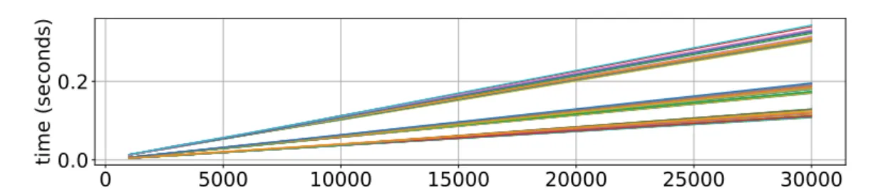
Figure 1. Time for inversion of all matrices on CPU using 1, 2 and 4 threads as function of batch size. Different colors correspond to different matrices

Next we use MAGMA library by calling magma (S/D)gesv batched routine that ex-ecutes the linear solution of systems on a GPU in single or double precision. MAGMA uses full matrix storage and we refer to magma library below as magma float and magma double, respectively, for single and double precision call.

We also test two cuSOLVER libraries. The first one is using QR matrix decomposition and is called by cusolver(S/D)pXcsrqrsvBatched routine in single or double precision. Some additional preparations must be made that analyse system matrices connectivity graph and transfer reordering permutations to increase the efficiency on the device, for more information we refer a reader to the manual [5]. The second one is called refactored solver that uses LU matrix decomposition and is called by cusolverRfBatchSolve routine. Note that some additional preparations must be made on a host part of the program. Besides, the interface of the call is assumed to be only in double precision (with respect to CUDA Toolkit Version 8.0). Both routines use sparse CRS matrix storage format. We refer to these libraries asQR float,QR double and RF double, respectively.

Our test is performed in the following manner. We generate a set of matrices with sizes

M =_{4,5,8,9,10,11,14,16_}with random sparsity patterns having filling 10%, 25% and 50% of all matrix elements, except diagonal elements. We also fill diagonal elements in such a way, that matrices are invertable. It is checked on the stage of matrix generation. We assume that pivoting can be used to these systems to increase the stability of system solution to perturbations. We use the following set of batch sizes: N =_{1,3,6,10,30,60,100,300,600,1000_{} ·}103_{. We also check}

the performance of two different GPUs with single and double precision calculations, where possible. The test set is generated as a tensor product of all possible configurations. For each test in the test set we make 10 runs of the code with different generated matrices that share the same sparsity pattern, and execution time is averaged. Performance is measured in FLOPS obtained from nvprof utility. All tests are generated, executed and logged by an automated Python script.

We used CPU device INTEL XEON E5-2609 2.4 GHz, 4 cores and two GPU devices. The first one designatedDevice 0is a GTX TITAN X NVIDIA card with 12 GB RAM, 11 TFLOPS peak single precision, 1/32 multiplier for double precision and 5.2 compute capability. The second

Device 1 is a GTX TITAN Black NVIDIA card with 6 GB RAM, 5.1 TFLOPS peak single precision, 1/3 multiplier for double presision and 3.5 compute capability.

2. Gauss–Jordan Elemiation Using Register Shuffle

0.0 0.5 1.0 1.5 2.0 2.5 3.0

batches

1e4

0.01

0.02

0.03

0.04

tim

e (

se

co

nd

s)

0.0

0.2

0.4

0.6

0.8

1.0

batches

1e6

0.00

0.05

0.10

0.15

tim

e (

se

co

nd

s)

All matrices

Figure 2. Time for inversion of all matrices on GPU using magma float (left) and QR float as function of batch size on Device 0. Different colors correspond to different matrices

0.0

0.2

0.4

0.6

0.8

1.0

batches

1e6

0.0

0.1

0.2

tim

e (

se

co

nd

s)

0.0

0.2

0.4

0.6

0.8

1.0

batches

1e6

0.00

0.05

0.10

0.15

tim

e (

se

co

nd

s)

All matrices

Figure 3. Time for inversion of all matrices on GPU using QR double (left) and RF as function of batch size on Device 0. Different colors correspond to different matrices

0.0 0.5 1.0 1.5 2.0 2.5 3.0

batches

1e4

1

2

3

4

5

rat

io

0.0 0.5 1.0 1.5 2.0 2.5 3.0

batches

1e4

10

20

30

40

rat

io

matrix_size:4

matrix_size:5

matrix_size:8

matrix_size:9

matrix_size:10

matrix_size:11

matrix_size:14

matrix_size:16

sparsity 0.5

0.0 0.5 1.0 1.5 2.0 2.5 3.0

batches

1e4

1

2

3

4

rat

io

0.0 0.5 1.0 1.5 2.0 2.5 3.0

batches

1e4

10

20

30

rat

io

matrix_size:4

matrix_size:5

matrix_size:8

matrix_size:9

matrix_size:10

matrix_size:11

matrix_size:14

matrix_size:16

sparsity 0.5

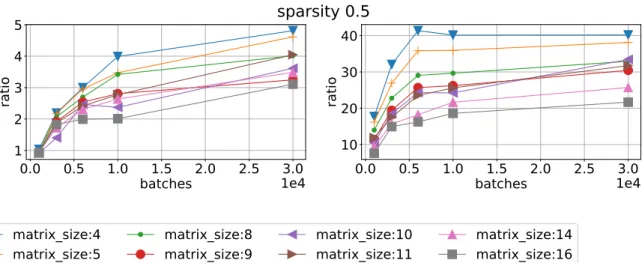
Figure 5.Ratio of mean time execution vs batch size using sparsity 0.5 for different matrix sizes. CPU/magma float left and CPU/QR float right on Device 1

0.0 0.5 1.0 1.5 2.0 2.5 3.0

batches

1e4

10

20

30

rat

io

0.0 0.5 1.0 1.5 2.0 2.5 3.0

batches

1e4

0

10

20

rat

io

matrix_size:4

matrix_size:5

matrix_size:8

matrix_size:9

matrix_size:10

matrix_size:11

matrix_size:14

matrix_size:16

sparsity 0.5

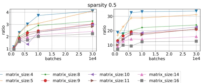
Figure 6.Ratio of mean time execution vs batch size using sparsity 0.5 for different matrix sizes. CPU/QR double left and CPU/RF right on Device 0

0.0 0.5 1.0 1.5 2.0 2.5 3.0

batches

1e4

10

15

20

25

rat

io

0.0 0.5 1.0 1.5 2.0 2.5 3.0

batches

1e4

5

10

15

20

rat

io

matrix_size:4

matrix_size:5

matrix_size:8

matrix_size:9

matrix_size:10

matrix_size:11

matrix_size:14

matrix_size:16

sparsity 0.5

0.0 0.5 1.0 1.5 2.0 2.5 3.0

batches

1e4

7.5

10.0

12.5

15.0

17.5

rat

io

0.0 0.5 1.0 1.5 2.0 2.5 3.0

batches

1e4

5.0

7.5

10.0

12.5

15.0

rat

io

matrix_size:4

matrix_size:5

matrix_size:8

matrix_size:9

matrix_size:10

matrix_size:11

matrix_size:14

matrix_size:16

sparsity 0.5

Figure 8.Ratio of mean time execution vs batch size using sparsity 0.5 for different matrix sizes. magma float/QR float left and magma double/QR double right on Device 0

0.0 0.5 1.0 1.5 2.0 2.5 3.0

batches

1e4

2

4

6

rat

io

0.0

0.2

0.4

0.6

0.8

1.0

batches

1e6

1.0

1.2

1.4

rat

io

matrix_size:4

matrix_size:5

matrix_size:8

matrix_size:9

matrix_size:10

matrix_size:11

matrix_size:14

matrix_size:16

sparcity 0.5

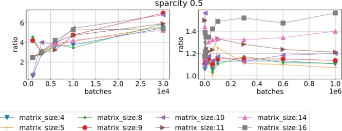
Figure 9.Ratio of mean time execution vs batch size using sparsity 0.5 for different matrix sizes. magma float/RF left and QR double/QR float right on Device 0

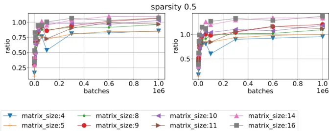
3.0 and above. It allows us to share data between threads that are part of the same warp. It insures a speedup of about 3 times to the shared memory access speed but limits current implementation in using only single precision arithmetics (double precision requires spliting into two 32b registers) and matrix size M _≤ W, where W is a warp size. For more information see [3, 6]. This code is now being tested and is in alpha version, we designate this code as

0.0

0.2

0.4

0.6

0.8

1.0

batches

1e6

0.25

0.50

0.75

1.00

rat

io

0.0

0.2

0.4

0.6

0.8

1.0

batches

1e6

0.5

1.0

rat

io

matrix_size:4

matrix_size:5

matrix_size:8

matrix_size:9

matrix_size:10

matrix_size:11

matrix_size:14

matrix_size:16

sparsity 0.5

Figure 10. Ratio of mean time execution vs batch size using sparsity 0.5 for different matrix sizes. QR float/RF left and QR double/RF right on Device 1

0.0

0.2

0.4

0.6

0.8

1.0

batches

1e6

0.0

0.2

0.4

0.6

0.8

rat

io

0.0

0.2

0.4

0.6

0.8

1.0

batches

1e6

0.0

0.5

1.0

rat

io

matrix_size:4

matrix_size:5

matrix_size:8

matrix_size:9

matrix_size:10

matrix_size:11

matrix_size:14

matrix_size:16

sparsity 0.5

3. Results

3.1. Libraries Analysis

All results are brought into figures that represent sections and projections of multidimen-sional data from the test set. All figures are self–explanationary, but we comment on some of most essential results. In Fig. 1 we can see the time needed to solve systems of equations for all matrices as function of batch size (up to 30,000 matrices) using 1,2 and 4 threads with single precision. We can see linear scaling with batch size since all matrices are treated as dense and have no dependence on sparsity. Analogous results by different libraries on Device 0 are provided in Fig. 2, 3 showing significant reduction of time. Interesting to note that batched RF method having no interface with single precision is almost as efficient as QR float. Results are a little bit different on Device 1. We checked the occupancy of GPU RAM. QR float and RF use about the same amount of RAM, for example it requires 1845 MB using QR float and 3590 MB using RF for N = 1·106, M = 11, and sparsity 0.5. MAGMA requires way more memory due to some internal memory allocation instructions, for example magma float takes about 831 MB for

N = 3·104, M = 11 and about 5264 MB forN = 2.4·105. This memory is dynamically allocated during the solution process and can cause exception of insufficient memory despite that memory for all matrices storage is sufficient, so we limit MAGMA batch size up to 30,000.

Speed ups against CPU 4-thread code for different libraries and different devices are shown in Fig. 4–7. We can see that MAGMA speed up varies from 5 to 3 times for Device 0 and 4 – 2 times for Device 1. QR float achieves speed up 40 times for small matrices and 20 for big matrices on Device 0 and 35 – 15 times for Device 1. RF is about the same results, lower by approximately 10% and QR double lower by another 10%. We can see that RF library has a narrower spread between matrix sizes.

We then benchmark one library against another in terms of execution time. Results for MAGMA library are presented in Fig. 8 and 9 (left). One can see that other libraries are faster, so taking memory demands into account we scratch out MAGMA from comparison. We also compare QR float and QR double with RF on different devices. We can see in Fig. 10 that RF version is more efficient on Device 1 compared with both QR double and QR float. However, QR float is more efficient on Device 0, see Fig. 11.

Further investigation is conducted in term of speed dependence from sparsity and matrix size for all batches. For this test we check only Device 0 because we found that the difference in scaling on these axes is negligible. One see the scaling of QR float on sparsity 0.1 in Fig. 12 and sparsity 0.5 in Fig. 13. The factor of speed loss is about 2 3 times for the matrix size increase from 4 to 16 when sparsity is 0.5 which implies better performance on bigger matrices. This effect is even stronger when sparsity is 0.1 and also for RF library, see Fig. 14 and 15. Another dependence on sparsity is given in terms of matrix size and provided for QR float in Fig. 18, 19, and for RF in Fig. 16, 17.

4

6

8

10 12 14 16

matrix size

10

10

10

tim

e (

se

co

nd

s)

4

6

8

10 12 14 16

matrix size

1.0

1.5

2.0

rat

io

batch_size:1000

batch_size:3000

batch_size:6000

batch_size:10000

batch_size:30000

batch_size:60000

batch_size:100000

batch_size:300000

batch_size:600000

batch_size:1000000

sparcity 0.1

Figure 12. Mean time execution (left) and ratio of time execution to the smallest matrix vs matrix size for different batch sizes and sparsity 0.1 using QR float on Device 0

4

6

8

10 12 14 16

matrix size

10

10

10

tim

e (

se

co

nd

s)

4

6

8

10 12 14 16

matrix size

1.0

1.5

2.0

2.5

rat

io

batch_size:1000

batch_size:3000

batch_size:6000

batch_size:10000

batch_size:30000

batch_size:60000

batch_size:100000

batch_size:300000

batch_size:600000

batch_size:1000000

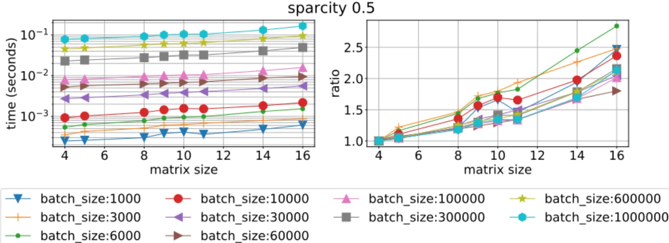
sparcity 0.5

Figure 13. Mean time execution (left) and ratio of time execution to the smallest matrix vs matrix size for different batch sizes and sparsity 0.5 using QR float on Device 0

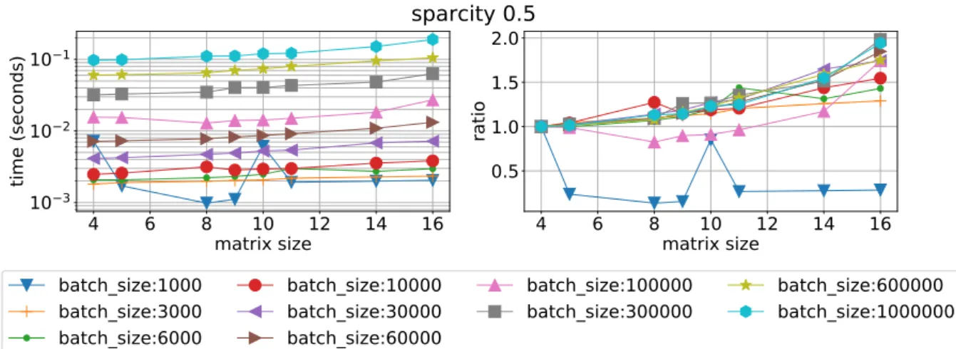
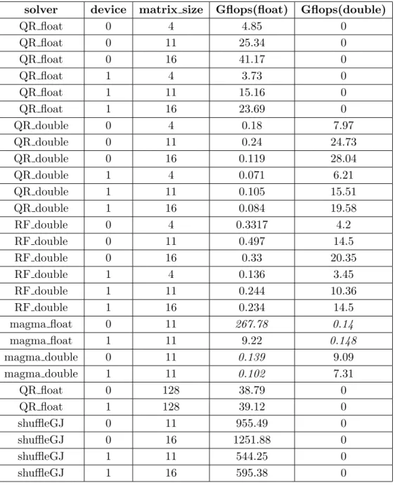
see, that QR float achieves maximum performance of 39.12 GFlops, so we can assume that the metrics is correct for M = 16. RF method also uses some single precision calculations but bulk part of all calculations is done in double precision with maximum of 20.35 GFlops.

3.2. Shuffle Gauss–Jordan Analysis

4

6

8

10 12 14 16

matrix size

10

10

10

tim

e (

se

co

nd

s)

4

6

8

10 12 14 16

matrix size

0.8

1.0

1.2

1.4

rat

io

batch_size:1000

batch_size:3000

batch_size:6000

batch_size:10000

batch_size:30000

batch_size:60000

batch_size:100000

batch_size:300000

batch_size:600000

batch_size:1000000

sparcity 0.1

Figure 14. Mean time execution (left) and ratio of time execution to the smallest matrix vs matrix size for different batch sizes and sparsity 0.1 using RF on Device 0

4

6

8

10 12 14 16

matrix size

10

10

10

tim

e (

se

co

nd

s)

4

6

8

10 12 14 16

matrix size

0.5

1.0

1.5

2.0

rat

io

batch_size:1000

batch_size:3000

batch_size:6000

batch_size:10000

batch_size:30000

batch_size:60000

batch_size:100000

batch_size:300000

batch_size:600000

batch_size:1000000

sparcity 0.5

Figure 15. Mean time execution (left) and ratio of time execution to the smallest matrix vs matrix size for different batch sizes and sparsity 0.5 using RF on Device 0

0.1

0.2

0.3

0.4

0.5

sparcity

10

10

10

tim

e (

se

co

nd

s)

0.1

0.2

0.3

0.4

0.5

sparcity

0.6

0.8

1.0

1.2

rat

io

batch_size:1000

batch_size:3000

batch_size:6000

batch_size:10000

batch_size:30000

batch_size:60000

batch_size:100000

batch_size:300000

batch_size:600000

batch_size:1000000

matrix size 8

0.1

0.2

0.3

0.4

0.5

sparcity

10

10

10

tim

e (

se

co

nd

s)

0.1

0.2

0.3

0.4

0.5

sparcity

1.00

1.25

1.50

1.75

rat

io

batch_size:1000

batch_size:3000

batch_size:6000

batch_size:10000

batch_size:30000

batch_size:60000

batch_size:100000

batch_size:300000

batch_size:600000

batch_size:1000000

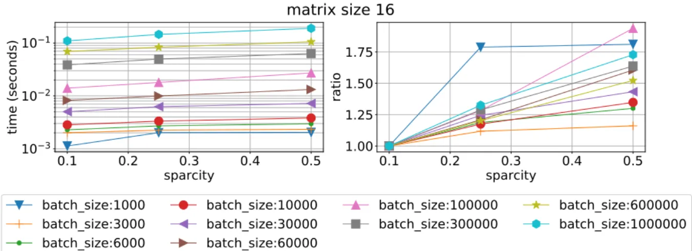
matrix size 16

Figure 17. Mean time execution (left) and ratio of time execution to the smallest sparsity vs sparsity fill for different batch sizes and matrix size 16 using RF on Device 0

0.1

0.2

0.3

0.4

0.5

sparcity

10

10

10

tim

e (

se

co

nd

s)

0.1

0.2

0.3

0.4

0.5

sparcity

1.0

1.1

1.2

rat

io

batch_size:1000

batch_size:3000

batch_size:6000

batch_size:10000

batch_size:30000

batch_size:60000

batch_size:100000

batch_size:300000

batch_size:600000

batch_size:1000000

matrix size 8

Figure 18. Mean time execution (left) and ratio of time execution to the smallest sparsity vs sparsity fill for different batch sizes and matrix size 8 using QR float on Device 0

0.1

0.2

0.3

0.4

0.5

sparcity

10

10

10

tim

e (

se

co

nd

s)

0.1

0.2

0.3

0.4

0.5

sparcity

1.0

1.2

1.4

1.6

rat

io

batch_size:1000

batch_size:3000

batch_size:6000

batch_size:10000

batch_size:30000

batch_size:60000

batch_size:100000

batch_size:300000

batch_size:600000

batch_size:1000000

matrix size 16

0.0

0.2

0.4

_batches

0.6

0.8

_1e6

1.0

10

15

20

25

rat

io

0.0

0.2

0.4

_batches

0.6

0.8

_1e6

1.0

10

10

rat

io

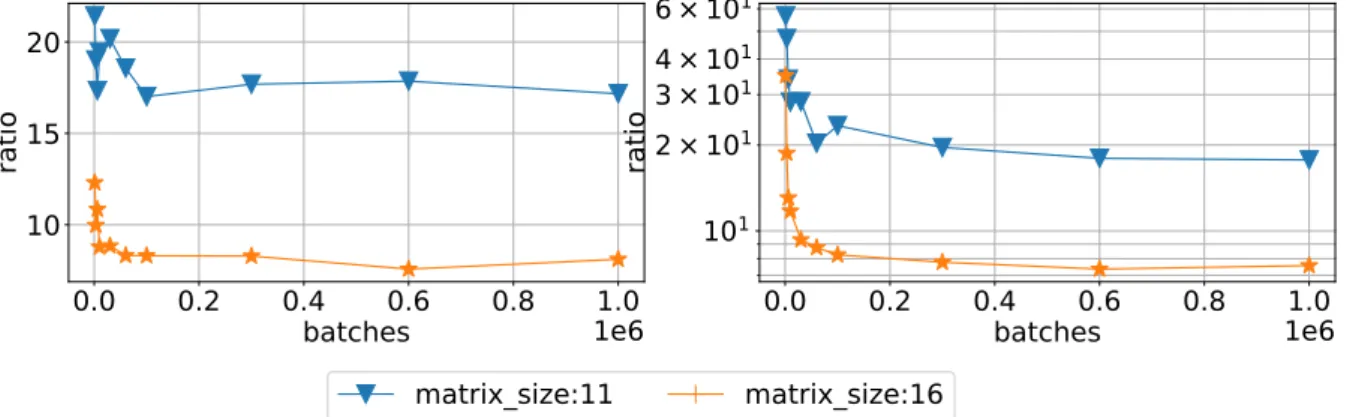
matrix_size:11

matrix_size:16

Figure 20. Ratio of time execution of QR float/shuffleGJ (left) and RF/shuffleGJ (right) as function of batch size for sparsity 0.5 on Device 0

0.0

0.2

0.4

0.6

0.8

1.0

batches

1e6

10

15

20

rat

io

0.0

0.2

0.4

0.6

0.8

1.0

batches

1e6

10

2×10

3×10

4×10

6×10

rat

io

matrix_size:11

matrix_size:16

Table 1.Performance of different batch solver

implementations on selected problems with sparsity 0.5 and one million batch size

solver device matrix size Gflops(float) Gflops(double)

QR float 0 4 4.85 0

QR float 0 11 25.34 0

QR float 0 16 41.17 0

QR float 1 4 3.73 0

QR float 1 11 15.16 0

QR float 1 16 23.69 0

QR double 0 4 0.18 7.97

QR double 0 11 0.24 24.73

QR double 0 16 0.119 28.04

QR double 1 4 0.071 6.21

QR double 1 11 0.105 15.51

QR double 1 16 0.084 19.58

RF double 0 4 0.3317 4.2

RF double 0 11 0.497 14.5

RF double 0 16 0.33 20.35

RF double 1 4 0.136 3.45

RF double 1 11 0.244 10.36

RF double 1 16 0.234 14.5

magma float 0 11 267.78 0.14

magma float 1 11 9.22 0.148

magma double 0 11 0.139 9.09

magma double 1 11 0.102 7.31

QR float 0 128 38.79 0

QR float 1 128 39.12 0

shuffleGJ 0 11 955.49 0

shuffleGJ 0 16 1251.88 0

shuffleGJ 1 11 544.25 0

Table 2.Performance of MAGMA 2.3 library for LU factorization and solution of linear systems on matrices 16_×16 with sparsity 0.5. Asterisk indicates tests with self written code, other tests use standard MAGMA library tests. Symbol ’—’ means that the problem does not fit in device memory

routine batch size _·103 _{Gflops time, ms}

sgetrf batched (LU) 100 282.21 0.93

sgetrf batched nopiv (LU) 100 2.08 30.03

sgesv batched (Solves) 100 14.67 20.0

sgetrs batched∗ (Solves with LU) 100 12.4 23.05

sgetrf batched (LU) 200 253.14 2.07

sgetrf batched nopiv (LU) 200 10.39 50.35

sgesv batched (Solves) 200 19.68 31.0

sgetrs batched∗ (Solves with LU) 200 18.3 33.86

sgetrf batched (LU) 500 258.09 5.07

sgetrf batched nopiv (LU) 500 31.18 41.95

sgesv batched (Solves) 500 22.63 72.9

sgetrs batched∗ (Solves with LU) 500 26.7 33.86

sgetrf batched (LU) 1000 307.26 8.51

sgetrf batched nopiv (LU) 1000 83.37 31.95

sgesv batched (Solves) 1000 — —

sgetrs batched∗ (Solves with LU) 1000 — —

3.3. Notes on MAGMA Library

We thank an anonymous reviewer for pointing out on the efficiency of newly released MAGMA 2.3 library (at the time of this research submission in October, 2017 latest MAGMA version was 2.2) for LU decomposition in batch mode. We performed tests on MAGMA library and confirmed that it achieves efficiency up to 308 GFlops (Device 0) for batched LU decom-position in single precision using magma sgetrf batched call with approximately 9.0 ms for one million matrices sized 16_×16. This is outstanding result compared to CUBLAS native NVIDIA library. However, in this papaer we are interested in batch solution of linear systems. So we testedmagma sgesv batchedandmagma sgetrs batchedroutines and obtained results close to the ones we obtained for MAGMA 2.2, see Tab. 2 for Device 0. For these tests we used simple programs that called these routines and compiled tests that are available in MAGMA library. Notice, that routine with no pivoting for LU decomposition takes substantial amount of time, compared to the standard LU decomposition with pivoting. This behaviour is abnormal and must be investigated.

calls are not optimally located for 1D indexing and one must introduce 2D grid in order to perform efficient solution of linear systems with sequential swaps in shared memory. This is the scope of the future work. More tests are required since results in paper [2] show performance of up to 800 GFlops for batch inversion of small matrices on P100 GPUs. Still, even LU MAGMA efficiency can’t outperform our implementation of Gauss–Jordan method, compare GFlops in Tab. 1 and Tab. 2 for matrices 16_×16 on Device 0.

4. Application Example

We are considering a standard chemical reaction flow benchmark problem, called ZND [9, 17, 18]. The problem is formulated for compressible perfect gas equations with chemical reaction. Detonation wave is propotaged with constant velocity D. The wave has the following structure: gas shock wave is propotaged, followed by reaction domain. Detonation reaction velocity is behind the shock wave. Governing equations are given bellow:

        

ρt+∇ ·(ρu) = 0,

(ρu)_t+_{∇ ·}(u_⊗(ρu)) +_∇p=0, ρEt+∇ ·(u(ρE+p)) = 0,

(ρYj)t+∇ ·(ρYju) = ˙ωj. ρE= 1₂ρu2_{+ρe, j= 1, M ,}

M

X

j=1

Yj = 1.

(2)

The chemical source term is given by:

˙

ω1 =−ω˙2 =

(

−ρY1Aexp −_RE_Tact

, T _≥Tign,

0, T < Tign.

(3)

Above equations are coupled by the equation of state:

p=ρRT,e

h=CpT+h0, h0 =PMj=1h0,jYj, Cp= _γ−γ₁R.e

(4)

Here ρis density of gas mixture, ρYj is the mass fraction of gas speciesj,M = 2 is the number

of species, A is the Arrhenius frequency factor,u is the velocity vector,p is the pressure, E is the total energy density, h is the specific enthalpy, e is the specific internal energy, ˙ωj is the

reaction rate of species j,T is temperature, _R= 8.31451 is the universal gas constant, Re = 1 is the specific gas constant, γ is the specific heat ratio of the gas mixture, h0,j is the reference

enthalpy of formation for the species j. In all calculations we set T = 1 and Tign = 1.01. The

fluid dynamics is solved using discontinuous Galerkin method [10], and the chemical part is solved using Crank–Nicolson method.

We define two domains – 1D segment and 2D plane. For the 1D segment we set boundary conditions as supersonic outflow conditions on the right and subsonic outflow conditions on the left. For the 2D plane we add two boundary conditions of sleep walls on top and bottom.

Initial conditions are defined as:

• x_≥0: (ρ, ρux, ρuy, ρE, ρY1, ρY2)T = (ρY1∗,−ρY1∗D,0, ρE, ρY1∗,0)T;

• x <0:

dY1(x)

dx =−

˙

ω(Y1(x))

ρ(Y1(x))Y1∗D

0

2

4

6

8

10

12

0

50

100

150

200

250

300

x

p

Figure 22. Pressure distributions for different time steps (10 seconds per step). Propagation velocity Dnum ∼3.664275 m/s

Here Y1 is burned species, and Y2 = 1−Y1 is unburned species, Y1∗ = 1 is a constant value.

All other values for initial conditions are calculated in accordance with [11] as functions of

Y1(x),∆h0,2, D. The Arrhenius frequency factor A is obtained from the given half–reaction

length of a detonation wave as:

L_1/2 =₋ρ2D

Z 1

1/2

1 ˙

ω(z)dz. (6)

The initial value problem (5) and value of A cannot be solved analytically, but the solution to these problems can be computed numerically for any given accuracy.

Three tests are performed – 1D comparison of computed velocity of detonation wave D, stability and instability of detonation wave for different initial D and 2D unstable detonation wave propagation. First results of the detonation wave propagation are presented in Fig. 22 for parameters γ = 1.4, L_1/2 = 12.5448 m. One can observe that the obtained velocity Dnum ∼

3.664275 m/s is close to the reference propagation velocity D = 3.66931 m/s. The other test verifies the stability of the detonation wave under provided value of D. We use parameter

f to define the propagation velocity D = √f DCJ from the analytical speed DCJ given by

the Chapman – Jouguet theory [11]. The results demonstrate that for L_1/2 = 1, γ = 1.4 and different values of parameterf one obtains different stability properties for the detonation wave. The results in Fig. 23 fully agree with reference results from [12].

The third test demonstrates spatial heterogeneity of the detonation wave (Fig. 24), calcu-lated for the same parameter values as the previous test. Again, we can check these results with reference data from [12].

55 60 65 70 75 80 85 90

0 10 20 30 40 50 60 70 80 90 100 110

f=1.6 f=2

t,sec p

4 5 6 7 8 9 10

0 20 40 60 80 100 120 140 160

f=1.6 f=2 x

ux

Figure 23. Temporal (left) and spatial (right) evolution of the detonation wave as function of initial detonation velocity parameter f

Figure 24. Spatial evolution ofρY1 for different time steps in the reference frame moving with

Table 3.Acceleration of the 2D ZND problem for reactive flow (chem) and pure gas dynamics (no chem).

solver time per step (ms) acceleration

CPU, 1 thread, chem 8,708.158 1.00

GPU, Device 0, chem 46.339 187.92

GPU, Device 1,chem 65.381 133.19

CPU, 1 thread, no chem 5,922.279 1.00 GPU, Device 0, no chem 27.935 212.00 GPU, Device 1, no chem 43.538 136.03

Conclusion

First, we wish to note that we do not recommend using MAGMA batch library call for the solution of the problem (1) at least for library version 2.2. It is clear from all metrics that we collected, especially from Tab. 1. We also notice that it is very inefficient to use MAGMA solution routines for both MAGMA 2.2. and MAGMA 2.3. However, one can benefit from using very efficient MAGMA LU factorisation and then solve the system manually. This combination may look promising if one is ready to implement a self-written routine. Also, MAGMA may work much more efficiently on cutting edge GPUs (VOLTA architecture) so one must try MAGMA on these GPUs as well.

For the available libraries we can conclude the following. It is beneficial to use RF method if your code uses double precision arithmetics and QR float if you are using single precision for our GPUs. This is valid for our hardware where GPUs have poor double precision performance. Both these methods perform graph connectivity analysis on CPU of provided matrices before calling batched routine for the solution of the problem on GPU. So these methods would require additional CPU work if your matrices connectivity is changing from one execution to anther. Note that the GFlops achieved by both of these methods is about 0.3 – 0.5% of the peak GFlops performance of GPUs.

If your GPUs support compute capability 3.0 and higher we can recommend using shuffle Gauss–Jordan method as an alternative to libraries for batch solution of linear systems. Achieved GLOPS and accelerations look promising. Debugging of this code and using it to solve plasma– chemistry on GPU is our next goal. Note, that we did not test this implementation on new NVIDIA GPUs (Volta architecture) and can’t extrapolate these results.

In the last section we demonstrate a successful application of the batched solver in the coupled gas dynamics reacting to flow ZND problem.

Benchmark source codes are availablable at github [13] under GPL licence.

Acknowledgments

This work is supported by RFBR grant no. 17-07-00116 and by subprogram 0063–2016–0018 of the program III.3 ONIT RAS.

References

1. Abdelfattah, A., Haidar, A., Tomov, S., Dongarra, J.: Performance, Design, and Auto-tuning of Batched GEMM for GPUs. In: Kunkel, J.M., Balaji, P., Dongarra, J. (eds.) High Performance Computing, pp. 21–38, Springer International Publishing, Cham (2016), DOI: 10.1007/978-3-319-41321-1 2

2. Abdelfattah, A., Haidar, A., Tomov, S., Dongarra, J.: Factorization and Inversion of a Million Matrices using GPUs: Challenges and Countermeasures. Procedia Computer Science 108, 606–615, (2017), DOI: 10.1016/j.procs.2017.05.250

3. Anzt, H., Dongarra, J., Flegar, G., Quintana-Orti, E.S.: Batched Gauss-Jordan Elimination for Block-Jacobi Preconditioner Generation on GPUs. In: PMAM’17 Proceedings of the 8th International Workshop on Programming Models and Applications for Multicores and Many-cores, 04–08 USA–February, Austin, TX, pp. 1–10 (2017), DOI: 10.1145/3026937.3026940 4. Asaithambi, R., Muppidi, S., Mahesh, K.: A numerical method for DNS of turbulent reacting

flows using complex chemistry. 42nd AIAA Fluid Dynamics Conference and Exhibit, AIAA 2012–3252, (2012), DOI: 10.2514/6.2012-3252

5. cuSOLVER CUDA Toolkit Documentation. http://docs.nvidia.com/cuda/cusolver/index.html, accessed: 2018-04-01

6. Demouth, J.: Shuffle: Tips and Tricks. GPU Technology conference, (2013). http://on-demand.gputechconf.com/gtc/2013/presentations/S3174-Kepler-Shuffle-Tips-Tricks.pdf, ac-cessed: 2018-04-01

7. Dong, T., Haidar, A., Luszczek, P., Harris, J.A., Tomov, S., Dongarra, J.: LU Factorization of Small Matrices: Accelerating Batched DGETRF on the GPU. In: IEEE 6th Intl Symp on Cyberspace Safety and Security, 2014 IEEE 11th Intl Conf on Embedded Software and Syst (HPCC,CSS,ICESS), (2014), DOI: 10.1109/HPCC.2014.30

8. Dong, T., Haidar, A.,Tomov, S., Dongarra, J.: A Fast Batched Cholesky Factorization on a GPU. In: Proc of 43-rd International Conference on Parallel Processing, 432–440 (2014), DOI: 10.1016/j.jocs.2016.12.009

9. Doring, W.: On detonation processes in gases. Annals of Physics 43, 421–436, (1943), DOI: 10.1002/andp.19434350605

10. Evstigneev, N.M., Ryabkov, O.I.: On The Development of High-Order Discontinuous Galerkin Method on 3D Unstructured Grid for Hyperbolic and Parabolic Problems Using Graphics Processors. In: Short Articles and Posters of the XI International Conference on Parallel Computational Technologies (PCT’2017), Kazan, 3–7 April 2017, pp. 63–77. Chelyabinsk, Publishing Center of the South Ural State University (2017)

11. Fickett, W., Davis, W.C.: Detonation, Theory and Experiment. Dover Publications (2000) 12. Geßner, T.: Dynamic Mesh Adaption for Supersonic Combustion Waves modeled with De-tailed Reaction Mechanisms. Doctoral Dissertation, Universitat Freiburg im Breisgau (2001) 13. GIT authors repository. https://github.com/oryabkov/cuda batch linsolvers test.git,

14. MAGMA Library documentation. icl.cs.utk.edu/magma, accessed: 2018-04-01

15. Masliah, I., Abdelfattah, A., Haidar, A., Tomov, S., Baboulin, M., et al.: High-Performance Matrix-Matrix Multiplications of Very Small Matrices. 2nd International Conference on Par-allel and Distributed Computing (Euro–Par 2016), Aug 2016, Grenoble, France. Springer, Lecture Notes in Computer Science, vol. 9833, pp. 659–671, (2016), DOI: 10.1007/978-3-319-43659-3

16. Rosenbrock, H.H.: Some general implicit processes for the numerical solution of differential equations. The Computer Journal 5(4), 329–330, (1963), DOI: 10.1093/comjnl/5.4.329 17. von Neumann, J.: Theory of detonation waves. In: A. J. Taub, editor, John von Neumann,

Collected Works, vol. 6. Macmillan, New York (1942)