SECONDARY ANALYSIS IN OUTCOME-DEPENDENT-SAMPLING DESIGNS
Yinghao Pan
A dissertation submitted to the faculty at the University of North Carolina at Chapel Hill in partial fulfillment of the requirements for the degree of Doctor of Philosophy in the
Department of Biostatistics in the Gillings School of Global Public Health.
Chapel Hill 2017
Approved by: Haibo Zhou Jianwen Cai Amy Herring
c 2017 Yinghao Pan
ABSTRACT
Yinghao Pan: Secondary Analysis in Outcome-Dependent-Sampling Designs
(Under the direction of Haibo Zhou and Jianwen Cai)
Outcome-dependent-sampling (ODS) schemes have long been used to reduce the cost for epidemiology studies. In ODS designs, one observes the exposure/covariates with a probability that depends on the outcome variable. Popular ODS designs include case-control for binary outcome, and case-cohort for time-to-event outcome. Most studies have multiple endpoints of interest in addition to the primary outcome. This means that investigators often need to reuse the already collected data to evaluate the association between a secondary outcome and the covariates. This is referred to as secondary analysis. However performing secondary analysis in ODS designs can be tricky as the ODS data is not representative of the general population. In this dissertation, we study how to correctly and efficiently conduct secondary analysis in ODS designs.
We consider analyzing a secondary outcome in case-cohort studies. We proposed a maximum estimated likelihood approach, where the likelihood is based on jointly modeling the time-to-failure outcome and the secondary outcome. It is shown that our proposed estimated likelihood estimator has greater statistical efficiency over two inverse probability weighted type estimators. We apply our method to a data from Sister Study.
weighted (IPW) and augmented inverse probability weighted (AIPW) estimating equations are proposed to conduct secondary analysis. Data from Collaborative Perinatal Project (CPP) is utilized to illustrate our method.
ACKNOWLEDGEMENTS
I would like to thank my advisors, Drs. Haibo Zhou and Jianwen Cai, for the guidance, advices, patience, and encouragement during my PhD study. I have learned tremendously under their direction. I would also like to thank Drs. Amy Herring, Matthew Longnecker, and Donglin Zeng for willing to serve on my dissertation committee, and their valuable comments and suggestions.
TABLE OF CONTENTS
LIST OF TABLES . . . x
LIST OF FIGURES . . . xi
CHAPTER 1: INTRODUCTION . . . 1
CHAPTER 2: LITERATURE REVIEW . . . 4
2.1 Outcome-Dependent-Sampling Designs . . . 4
2.1.1 Statistical Methods for Case-control Design . . . 4
2.1.2 Statistical Methods for ODS Scheme with a Continuous Outcome . . 5
2.1.3 Statistical Methods for Case-cohort Design . . . 9
2.1.4 Statistical Methods for ODS Scheme with a Failure Outcome . . . 13
2.2 Secondary Analysis in ODS Designs . . . 15
2.2.1 Naive Analysis . . . 16
2.2.2 Inverse Probability Weighting . . . 17
2.2.3 Likelihood-based Methods . . . 17
2.2.4 Estimating Equation . . . 21
2.3 Semiparametric Inference Methods . . . 23
2.3.1 Augmented Estimating Equation . . . 23
2.3.2 Estimated Likelihood . . . 24
2.3.3 Empirical Likelihood . . . 25
2.4 Outline of Proposed Work . . . 26
2.4.2 Secondary Analysis for Data from an Outcome-Dependent
Sampling Design . . . 29
2.4.3 Efficient Secondary Analysis of Data from Two-Phase Studies . . . . 31
CHAPTER 3: REGRESSION ANALYSIS FOR SECONDARY RESPONSE VARIABLE IN A CASE-COHORT STUDY . . . 35
3.1 Introduction . . . 35
3.2 Data Structure and Model . . . 37
3.3 Estimated Likelihood Approach . . . 39
3.4 Derivation of Two New IPW Type Estimators . . . 43
3.5 Simulation Studies . . . 45
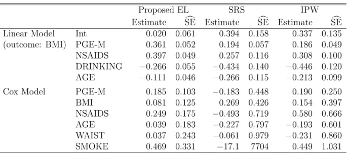
3.6 Analysis of Sister Study Data . . . 52
3.7 Discussion . . . 53
CHAPTER 4: SECONDARY ANALYSIS FOR DATA FROM AN OUTCOME-DEPENDENT SAMPLING DESIGN . . . 56
4.1 Introduction . . . 56
4.2 Data Structure and Model . . . 58
4.3 Estimating Equation Approach . . . 60
4.3.1 Inverse Probability Weighted Estimating Equation . . . 60
4.3.2 Augmented Inverse Probability Weighted Estimating Equation . . . 61
4.4 Asymptotic Results . . . 63
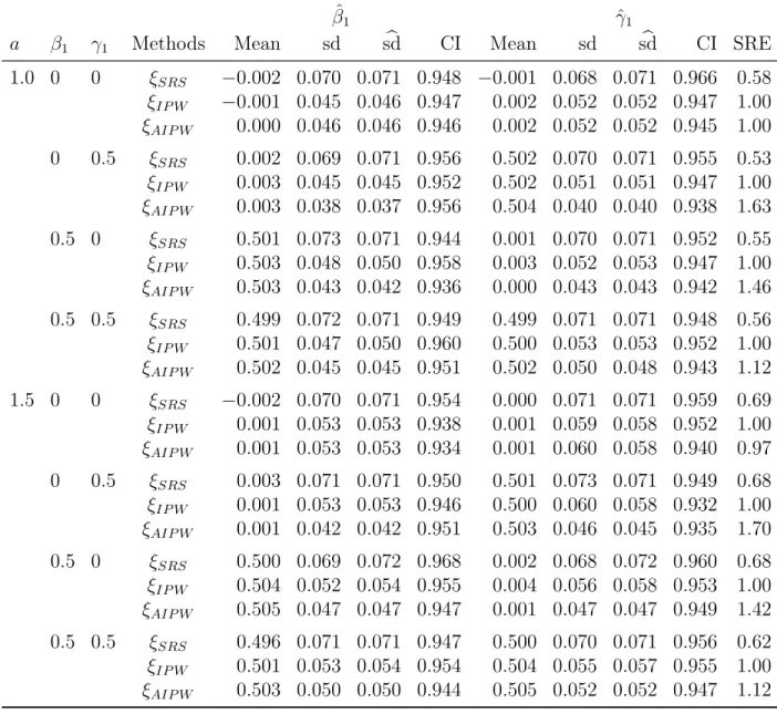
4.5 Simulation Studies . . . 64
4.6 Collaborative Perinatal Project Data . . . 71
4.7 Discussion . . . 75
4.8 Supplementary Materials . . . 76
CHAPTER 5: EFFICIENT SECONDARY ANALYSIS OF DATA FROM TWO-PHASE STUDIES . . . 78
5.1 Introduction . . . 78
5.2.1 Design and Data Structure . . . 80
5.2.2 Semiparametric Maximum Likelihood Inference . . . 82
5.2.3 Asymptotic Results . . . 84
5.3 Numerical Studies . . . 86
5.3.1 Derivation of an IPW estimator for Secondary Analysis . . . 86
5.3.2 Simulation Studies . . . 86
5.4 Analysis of the MoBa Study Data . . . 91
5.5 Concluding Remarks . . . 93
CHAPTER 6: SUMMARY AND FUTURE RESEARCH . . . 96
APPENDIX A: . . . 99
A.1 Appendix for Chapter 3 . . . 99
A.2 Appendix for Chapter 4 . . . 103
A.3 Appendix for Chapter 5 . . . 105
LIST OF TABLES
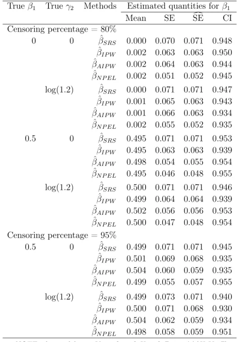
3.1 Simulation results with full cohort sizeN = 1000, the SRS sample
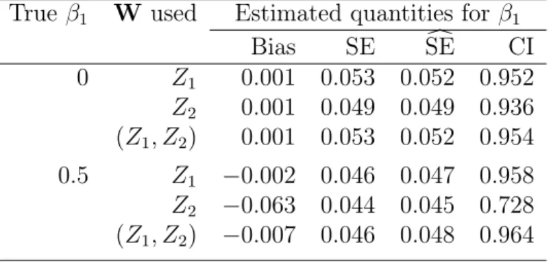
size is nSRS = 200. X ∼N(0,1), Z ∼Bernoulli(0.45). . . 47 3.2 Performance of our proposed estimatorβˆN P EL when we misspecify
W. Z = (Z1, Z2), where Z1 ∼Bernoulli(0.45), Z2 ∼Bernoulli(0.6).
X ∼N(Z1,1), which means that Z1 is the informative components
of Z about X. The true W is Z1. . . 50
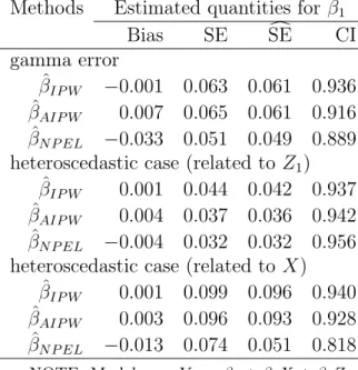
3.3 Simulation results when is not normal. β1 = 0.5. Z = (Z1, Z2),
where Z1 ∼Bernoulli(0.45),Z2 ∼Bernoulli(0.6), X ∼N(Z1,1). . . 51
3.4 Analysis of Sister Study. . . 53
4.1 Simulation results based on 1000 simulations withn0 = 200,
n1 =n3 = 100, the validation sample size is nV = 400, the
full cohort size is N = 3000. . . 66 4.2 Simulation results based on 1000 simulations withn0 = 300,
n1 =n3 = 50, the validation sample size is nV = 400, the
full cohort size is N = 3000. . . 67 4.3 Simulation results when is not normal. The full cohort size
isN = 3000, (n0, n1, n3) = (200,100,100). . . 72
4.4 Analysis for a secondary outcome: children’s birth weight in CPP study . . . 74 4.5 Simulation results based on 1000 simulations withn0 = 850,
n1 =n3 = 100, the validation sample size is nV = 1050, the
full cohort size is N = 40000. . . 77
5.1 Simulation results, secondary analysis for two-phase SODS design.
The full cohort size is N = 2500. The error term is normally distributed. . . 88 5.2 Simulation results when the error term is not normally distributed.
The full cohort size is N = 2500, (n0, n1, n3) = (500,50,50). . . 92
LIST OF FIGURES
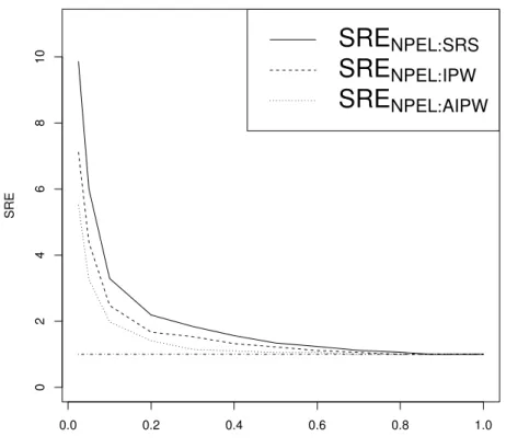
3.1 SREs comparing various estimators, under 80% censoring. . . 48 3.2 SREs comparing βˆN P EL to βˆSRS, under various censoring percentage. . . 49
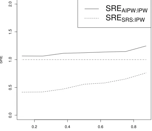
4.1 SREs comparing ξˆAIP W and ξˆSRS toξˆIP W in terms of estimating γ1,
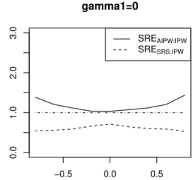
under various combinations of SRS and supplemental samples. . . 69 4.2 SREs comparing ξˆAIP W and ξˆSRS toξˆIP W in terms of estimating γ1,
under different values of ρ. . . 70
5.1 SREs comparing ξˆP toξˆSRS and ξˆIP W in terms of estimating β1,
CHAPTER 1: INTRODUCTION
If time and resources permitted, investigators would like to collect all the data on every member in a study population. However, this is usually not the case as large epidemiology studies typically require recruiting thousands of subjects and long time to follow up. Most of the costs and efforts come from collecting covariate information. In many studies, the primary outcome variable is easy to obtain, while some exposure variables are expensive to measure. This motivates statisticians to develop outcome-dependent-sampling (ODS) designs. In such designs, the probability of observing the exposure/covariate for a subject depends on the observed value of the outcome variable. By oversampling certain subjects, ODS design allows investigators to concentrate the resources on the segment of the population that are most informative in explaining the outcome/exposure relationship. ODS designs, coupled with appropriate analysis, provides more efficient estimates than standard statistical analysis based on a simple random sample.
For studies with binary outcome (i.e. the disease occurrence status), case-control design has been widely used since Cornfield (1951). When the disease is rare, much of the information collected on disease free subjects is redundant. Case-control design addresses this issue by oversampling the cases. The case-cohort design (Prentice, 1986) is another well known cost-effective ODS design used to study the determinants of a time-to-event outcome. Other ODS designs include generalized case-cohort design (Chen, 2001; Cai and Zeng, 2007), ODS scheme for continuous outcome (Zhou et al. 2002), survival outcome-dependent sampling (SODS) scheme for failure-time data (Ding et al. 2014) and so on. We will review them in
detail in the next chapter.
relationship between the covariates and a secondary outcome. This is referred to as secondary analysis. When the original data is a simple random sample of the general population, standard analysis methods can be used. However, when the original data is collected in an outcome-dependent way, secondary analysis can be challenging. As the data obtained from ODS designs is no longer a random representative of the general population, a naive approach ignoring the outcome-dependent sampling scheme will yield biased results. There has been extensive work focusing on secondary analysis in case-control studies, which will be reviewed later in the next chapter. However, up to my knowledge, there has been few research on secondary analysis in case-cohort study, and there is no existing work on secondary analysis in other types of ODS designs, such as the continuous outcome ODS scheme (Zhou et al. 2002) and the general ODS scheme for failure-time data (Ding et al. 2014). Our research is intended to fill these gaps.
Our research is motivated by several real data examples. Sister Study (Kim et al., 2011, 2013) is one study that adopts the case-cohort design. The Sister Study targets US women who have a sister with breast cancer, but with no breast cancer themselves at the start of the study. In this study, the primary time-to-event outcome is time to diagnosed breast cancer, and the expensive exposure variable is PGE-M, a major prostaglandin E2 metabolite. Because lab analysis of PGE-M level is costly, the exposure variable PGE-M is only measured in a simple random sample plus all those subjects who developed the breast cancer during the follow up. After studying the primary endpoint (time to breast cancer), investigators might be interested in investigating the relationship between a secondary outcome (BMI in this case) and the main exposure (PGE-M). Instead of designing and implementing a new study, investigators would prefer to re-use the existing Sister Study data to study the link between BMI and PGE-M, considering the tremendous cost and efforts involved in collecting the exposure variable.
polychlori-nated biphenyls (PCBs) in relation to children’s IQ performance. A continuous outcome ODS scheme is implemented as ascertainment of PCB level is expensive. PCB level is measured only for a simple random sample and two supplemental samples taken from two tails of the IQ performance. With the collected CPP data set, investigators might want to re-use it to explore the association between the PCB level and a secondary outcome (children’s birth weight).
CHAPTER 2: LITERATURE REVIEW
In this chapter, we review all the literatures related to our topic, and outline our proposed work.
In section 2.1, we review the literatures on four types of cost-effective ODS designs: 1)
case-control design. 2) ODS scheme with a continuous outcome discussed in Zhou et al. (2002). 3) case-cohort design. 4) ODS scheme for failure-time data proposed by Ding et al. (2014). All the papers we reviewed in this section focus on evaluating the association between
the exposure variable and the primary outcome variable (for which the sampling scheme is based on). In section 2.2, we review the existing work on analyzing a secondary outcome under ODS designs. In section 2.3, we review three frequently used semiparametric inference methods: augmented estimating equation, estimated likelihood and empirical likelihood. These methods will be used in our proposed work. We conclude this chapter by outlining the proposed work in section 2.4.
2.1 Outcome-Dependent-Sampling Designs
2.1.1 Statistical Methods for Case-control Design
the prospective and retrospective models lead to identical maximum likelihood estimates of the odds ratios for case-control data. This means that standard logistic regression could be applied to the case-control study as if the data had been obtained in a prospective study.
There are several extensions of case-control design. White (1982) proposed a two-stage design especially for a rare disease and a rare dichotomous exposure variable. In the first stage, the disease and exposure status are ascertained on a relatively large sample. The design for this stage could be case-control, or a cohort study. Then in the second stage, simple random samples are drawn within the four groups: two case groups (diseased and exposed/unexposed) and two control groups (non-diseased and exposed/unexposed), and other covariates are measured on these four random subsamples. When the disease and exposure is rare, four groups would have quite different sizes. The observations from the small groups will have more information than observations from the larger groups. Hence, this two stage design will be more efficient than a similar one stage design. Breslow and Cain (1988) considers the two-stage case-control study, and proposed a modified logistic regression.
In the first stage, disease status and easy to obtain covariates are obtained for a large number of subjects. Then in the second stage, expensive exposure is measured for a case-control sample from the general population. Flanders and Greenland (1991) showed how to use pseudo-likelihood approach to analyze two stage case-control data. Zhao and Lipsitz (1992) reviewed twelve two-stage designs, which include two-stage case-control and case-cohort as special case.
2.1.2 Statistical Methods for ODS Scheme with a Continuous Outcome
In many studies, the primary outcome is measured on a continuous scale. In order to implement a cost-effective design, investigators usually dichotomize the continuous outcome based on whether it is above or below a certain cut off point. However, some efficiency is lost by converting a continuous outcome into dichotomous scale. The choice of the cut off point is also subjective, which makes the results incomparable between different studies.
with a continuous outcome. Let Y be the primary outcome, and X be the vector of covariates. Assume that the domain of Y can be partitioned intoK mutually exclusive strata, Ck = (ak−1, ak], k= 1, . . . , K, where ak, k = 0,1, . . . , K are pre-fixed constants that satisfy −∞=a0 < a1 < a2 <· · ·< aK =∞. In the ODS design, a simple random sample of size n0
is selected from the full cohort, and then supplemental samples of size nk is chosen from each of the kth stratum: Ck, k= 1, . . . , K. LetN be the size of the full cohort, and let nV be the size of the ODS sample. Then, nV =PKk=0nk. According to measurement error literature, the ODS sample is called the validation sample, as we observed (Y, X)on these nV subjects. Let nV¯ = N −nV, then these nV¯ subjects for whomX is not observed are referred to as the
nonvalidation sample. In addition, let S0, Sk, k = 1, . . . , K be the index set of the simple random sample, and the supplemental samples, respectively. ThenV =∪K
k=0Sk is the index set of the validation sample (ODS sample). Zhou et al. (2002) used only the validation sample to develop the likelihood function.
Let fβ(y | x) be the conditional density of Y given X, and let GX and gX denote the cumulative distribution and density function of X, respectively. Also, F(u) =P r(Y ≤ u)
and F(u|x) =P r(Y ≤u|x). Then the likelihood function for the validation sample is
L(β, GX) = (
Y i∈S0
fβ(yi |xi)gX(xi) ) × " K Y k=1 Y j∈Sk
fβ(yj, xj |yj ∈Ck) #
=
( Y i∈S0
fβ(yi |xi)× K Y k=1
Y j∈Sk
fβ(yj |xj)
F(ak |xj)−F(ak−1 |xj) )
× (
Y i∈S0
gX(xi)× K Y k=1
Y j∈Sk
[F(ak|xj)−F(ak−1 |xj)]gX(xj) F(ak)−F(ak−1)
)
= L1(β)×L2(β, gX). (2.1)
misspecification, as covariates X could be high-dimensional. In their paper, the empirical likelihood approach is adopted (Owen. 1988, 1990; Vardi, 1985). They choose to leave GX unspecified and obtain an empirical likelihood function of GX over all distributions whose support contains the observed X values in the ODS sample.
Weaver and Zhou (2005) took an estimated likelihood approach for the regression analysis under continuous outcome ODS design. They made an attempt to incorporate the information in the non-validation sample, as the primary outcome Y is often measured for all the observations. The full sample likelihood is proportional to
LF(β, GX) = "
Y i∈V
fβ(Yi |Xi) #
· "
Y i∈V
dGX(Xi) #
·
Y j∈V¯
fY(Yj;β)
, (2.2)
where fY(y;β) is the marginal density of Y, i.e. fY(y;β) = R
fβ(y | x)dGX(x). Let Nk be the number of observations in the full cohort that belong to the kth stratum, n0,k is defined likewise for the SRS sample. In addition, let Vk represent the index set of the observations in the validation sample that belong to kth stratum. Then there arenk+n0,k observations in the index set Vk. It is known that
GX(x) =P r{X ≤x}= K X k=1
P r{Y ∈Ck}P r{X ≤x|Y ∈Ck}.
Weaver and Zhou (2005) proposed to use the followingGˆX(x)to consistently estimateGX(x), the distribution function of X:
ˆ
GX(x) = K X k=1 Nk N ˆ
Gk(x),where Gˆk(x) = X i∈Vk
I{Xi ≤x} nk+n0,k
.
Then it is possible to consistently estimate the marginal density of Y with the following estimator:
ˆ
fY(Yj;β) = K X
k=1
Nk N(nk+n0,k)
X i∈Vk
Replacing (2.3) into (2.2), and perform a log transformation, we have the following estimated log-likelihood:
ˆ
lF(β) =lF(β,GˆX) = "
X i∈V
logfβ(Yi |Xi) #
+
X j∈V¯
log
( K X k=1
Nk N(nk+n0,k)
X i∈Vk
fβ(Yj |Xi) )
.
The proposed estimator is obtained from maximizing this estimated likelihood. Estimated likelihood method can be traced back to Pepe and Fleming (1991) and Carroll and Wand (1991). The general idea is to nonparametrically estimate some components of the likelihood function (often a distribution function or a conditional distribution function) using the validation sample.
Song et al. (2008) showed that ODS design with a continuous outcome can be viewed as a natural extension of the two-stage case-control design to the continuous outcome case. Same as Weaver and Zhou (2005), the likelihood function for the full sample is
LF(β, GX) =
" Y i∈V
fβ(Yi |Xi)gX(Xi)
# ·
Y j∈V¯
Z
fβ(Yj |x)dGX(x)
. (2.4)
Song et al. (2008) developed a semiparametric efficient estimator for this setting. Replace g(Xi)with gi, the aim is to maximize the following log-likelihood:
lF(β, gi) = X
i∈V
logfβ(Yi |Xi) + X
i∈V
loggi+ X j∈V¯
log
( X i∈V
gifβ(Yj |Xi) )
,
under the constraint that P
i∈V gi = 1. Lagrange multiplier can be invoked.
vector of other covariates. Then the partial linear model has the following form:
E(Y |X, Z) =g(X) +ZTγ, (2.5)
where g(·)is an unknown smooth function. Zhou et al. (2011a) derived a penalized likelihood based on the validation sample data assuming that g(·) is a spline function. Qin and Zhou (2011) also studied the partial linear model under the same ODS design. But they incorporated the non-validation sample information into the likelihood. Zhou et al. (2011b) proposed a two-stage outcome-auxiliary-dependent sampling design (OADS). Suppose W is an auxiliary variable for the exposure X, meaning that W provides no additional information about Y when X and Z are known. The OADS design is as follows: In the first stage, outcomeY, auxiliary variable W, and other covariates Z are observed for all individuals. In the second stage, expensive exposure X is measured on a simple random sample and supplemental samples chosen from each stratum based on the partition of the domain of Y ×W. An estimated likelihood method is developed for this OADS design. Another recent development is the probability dependent sampling (PDS) design proposed by Zhou et al. (2014). Same as in ODS, an SRS sample is selected from the general population in the first stage. Before obtaining supplemental samples, a model for E(X |Y, Z)is fitted using the first phase simple random sample. In the second stage, supplemental samples are drawn from those whose X values are more likely to be in the two tails. Based on the likelihood for validation sample, Zhou et al. (2014) used an empirical likelihood procedure. It is shown that PDS design, with appropriate analysis will lead to more efficient estimates than ODS designs.
2.1.3 Statistical Methods for Case-cohort Design
the failure timeT˜ given possibly time-dependent covariates Z(·) has the following form:
λ(t|Z(t)) = λ0(t) exp{β
0
Z(t)}, (2.6)
where λ0(t)is the unspecified baseline hazard function, and β is the parameter of interest. Let C be the censoring time. For right-censored failure time data, what we observe is T = min( ˜T , C), and ∆ =I( ˜T ≤C), the failure indicator. Using counting process approach, letN(t) =I(T ≤t,∆ = 1) and let Y(t) =I(T ≥t) be the at-risk process. We assume that the failure time T˜ and censoring time C are conditionally independent given Z. Then for a cohort of n independent observations on the triplets (T,∆, Z), partial likelihood (Cox, 1972, 1975) is given by
L(β) =
n Y i=1 Y t≥0 (
exp(β0Zi(t)) Pn
j=1Yj(t) exp(β
0
Zj(t))
)∆Ni(t)
,
where ∆Ni(t) = 1 if the ith subject fails at time t, and 0 otherwise. Then the log-likelihood function is
l(β) =
n X i=1 Z ∞ 0 (
β0Zi(t)−log n X
j=1
Yj(t) exp(β
0
Zj(t)) !)
dNi(t).
Letτ be the end of the follow up period such that P r(Y(τ) = 1)>0, then the score equation can be written as
U(β) =
n X
i=1
Z τ
0
{Zi(t)−E(β, t)}dNi(t), (2.7)
where E(β, t) = S(1)(β, t)/S(0)(β, t) and S(0)(β, t) = n1 Pni=1Yi(t) exp(β
0
Zi(t)), S(1)(β, t) =
1
n Pn
i=1Zi(t)Yi(t) exp(β
0
Zi(t)). E(β, t)can be viewed as an empirical average of the covariates. The parameter of interest β can be estimated by the root of the score equation (2.7).
a simple random sample of the full cohort and on all the failure individuals. For case-cohort data, (2.7) cannot be calculated, because calculation of E(β, t) involves unobserved data. Hence, the risk set for each failure time needs to be modified. Prentice (1986) proposed the following pseudo-score equation:
U(β) =
n X i=1 Z τ 0 (
Zi(t)− P
j∈R˜(t)Zj(t)Yj(t) exp(β
0
Zj(t)) P
j∈R˜(t)Yj(t) exp(β
0
Zj(t)) )
dNi(t), (2.8)
whereR˜(t) =D(t)∪C. C represents the random subcohort, andD(t) ={i|Ni(t)6= Ni(t−)}. D(t) is the index set of the subjects who fail at time t. In other words, the risk set at each time tcontains all subcohort members at risk at timet and any subject outside the subcohort that fails at time t. As the filtration is not nested, standard martingale convergence results by Anderson and Gill (1982) can not be applied directly. A combination of martingale and finite population convergence results need to be used to rigorously derive the asymptotic properties. This is discussed in detail in Self and Prentice (1988).
Self and Prentice (1988) proposed another pseudo-score equation by setting R˜(t) = C. This means that only random subcohort members are included in the risk set. Compared to Prentice (1986), the risk set is slightly different. However, it can be shown that these two estimators are asymptotically equivalent as any individual’s contribution to S(1) andS(0) are
asymptotically negligible.
Variance computation for the pseudo-likelihood estimator (Prentice, 1986; Self and Prentice, 1988) is very complicated. Wacholder et al. (1989) developed a bootstrap estimate of the variance. But their approach is quite computationally intensive. Barlow (1994) and Lin and Ying (1993) proposed other variance estimators that can be computed more easily. Barlow (1994) also proposed a slightly different pseudo-likelihood compared to Prentice (1986) and Self and Prentice (1988). In his pseudo-score equation, a time-dependent weightw(t)is used:
U(β) =
n X i=1 Z τ 0 (
Zi(t)− Pn
j=1Zj(t)Yj(t)wj(t) exp(β
0
Zj(t))
Pn
j=1Yj(t)wj(t) exp(β
0
Zj(t)) )
where wi(t) =dNi(t) +{1−dNi(t)}ξim(t)/m˜(t), m(t) is the number of individuals in the full cohort at risk at time t, m˜(t) is the number of individuals in the random subcohort that is at risk at time t, ξi is the indicator of being in the random subcohort C for ith subject. This means that for a subject in the random subcohort (ξi = 1) that does not fail at time t (dNi(t) = 0), the weight received ism(t)/m˜(t). This is different from Prentice (1986), in which subcohort members will always receive weight 1.
Chen and Lo (1999) derived a class of estimating equations for the case-cohort design. The general idea is that while constructing the risk set, the information in all case samples should be used. Hence, their estimator has improved efficiency over the pseudo-likelihood estimator of Prentice (1986) and Self and Prentice (1988). The pseudo-score equation for Prentice (1986) is
U(β) =
n X
i=1
Z τ
0
(
Zi(t)− P
j∈R˜(t)Zj(t)Yj(t) exp(β
0
Zj(t)) P
j∈R˜(t)Yj(t) exp(β
0
Zj(t)) )
dNi(t). (2.10)
Notice that the second term in (2.10) estimate m(t), the conditional expectation ofZ given T =t and ∆ = 1. It is known that
E(Z |T =t,∆ = 1) = E(Ze
β0ZI
(T≥t))
E(eβ0ZI
(T≥t))
= pE(Ze
β0ZI
(T≥t)|∆ = 1) + (1−p)E(Zeβ
0
ZI
(T≥t)|∆ = 0)
pE(eβ0ZI
(T≥t)|∆ = 1) + (1−p)E(eβ
0
ZI
(T≥t)|∆ = 0)
, (2.11)
where p = P r(∆ = 1). Let pˆbe a consistent estimator of p, and replace the conditional expectations in (2.11) by the empirical estimates, it is possible to obtain a class of consistent estimators for m(t). As discussed in Chen and Lo (1999), suppose that R1 is the index set
of a random sample of k1 cases and R0 is the index set of a random sample of k0 controls.
LetR1
following estimating equation can be constructed:
X i∈R1
Z τ
0
Zi(t)−
(ˆp/k1)
P j∈R1
t Zj(t)e
β0Zj(t)+{(1−pˆ)/k
0}
P j∈R0
t Zj(t)e
β0Zj(t)
(ˆp/k1)Pj∈R1
t e
β0Zj(t)+{(1−pˆ)/k
0}Pj∈R0
t e
β0Zj(t)
dNi(t) = 0. (2.12) Based on (2.12), Chen and Lo (1999) proposed a class of estimators that apply to different situations of case-cohort design.
Other research work related to case-cohort design includes the following: Chen (2001) improved the pseudo-likelihood estimator by finding an optimal sample reuse method via local averaging. Borgan et al. (2000) considered stratified case-cohort design, and showed that the stratified case-cohort design were more efficient than a randomly sampled case-cohort study. Kulich and Lin (2004) developed a general class of doubly weighted estimator with time-varying weights under the stratified case-cohort designs, which includes Chen and Lo (1999), Borgan et al. (2000, est. II) and Chen (2001) as special cases. Kang and Cai (2009) extended the weighted estimating equation approach to generalized case-cohort study with multiple disease outcomes. They use marginal proportional hazards regression models to deal with correlated multiple disease outcomes. Kim et al. (2013) further improved the efficiency of estimators in case-cohort design with multiple disease outcomes. The general idea of their work is to use the covariate information from cases of all types in constructing the weight function.
2.1.4 Statistical Methods for ODS Scheme with a Failure Outcome
data with right censoring. In this ODS design, in addition to a simple random sample, supplemental cases are selected from different strata of the observed failure time. This ODS design has more efficiency over the generalized case-cohort design, as it allows investigators to oversample certain more informative failure subjects.
Ding et al. (2014) used an empirical likelihood approach to estimate the hazard ratio parameters for data collected from this failure-time ODS design. LetT˜ be the primary failure time of interest, and C be the censoring time. Also, let T =min( ˜T , C)be the observed time,
∆ =I( ˜T ≤ C) be the event indicator, and Z be a p-dimensional covariate. It is assumed that T˜ and C are conditionally independent given Z.
Suppose that the failure time T˜ follows the Cox proportional hazards model (Cox, 1972):
λ(t|Z) = λ0(t) exp(β
0
Z),
whereλ0(t)is the unspecified baseline hazard function, andβis the parameter of interest. Letτ
be the largest observed time of all the cases. The interval(0, τ]can be divided intoK mutually exclusive strata: Ak = (ak−1, ak], k = 1, . . . , K, where 0 = a0 < a1 <· · · < aK−1 < aK = τ. Ding et al. (2014) considers the following ODS design: In the first phase, a simple random sample (SRS) of size n0 is chosen from the full cohort of size N. In the second phase,
supplemental cases of sizenk are selected from each of the above kth stratum: Ak. Sample sizes nk, k= 0, . . . , K are constants fixed by design. To fix notation, let V, S0,and Sk be the index set of the overall ODS sample, simple random sample, and supplemental cases from the kth stratum, respectively. Then, V =∪K
k=0Sk. Using measurement error literature, V is called the validation sample. The failure-time outcome (T,∆) is observed for all subjects in the population, but the expensive exposure is measured only in the validation sample (the ODS sample).
the conditional density function. The likelihood function corresponding to the validation sample is the following:
L(β, QZ) = h Y
i∈S0
f(Ti,∆i |Zi)qZ(Zi) ihYK
k=1
Y i∈Sk
f(Ti,∆i, Zi|∆i = 1, Ti ∈Ak) i
. (2.13)
Let fβ,Λ0(t|Z) and F¯β,Λ0(t|Z)be the conditional density function and survival function
of T˜ given Z. In addition, let sC(t) and SC(t) be the density and survival function of the censoring timeC. Then it can be shown that the likelihood function (2.13) is proportional to
L(β, QZ,Λ0, SC) =
h Y i∈S0
(fβ,Λ0(Ti |Zi))∆i( ¯Fβ,Λ0(Ti |Zi))1−∆i i ·h K Y k=0 Y i∈Sk
qZ(Zi) i ·h K Y k=1 Y i∈Sk
fβ,Λ0(Ti |Zi) i ·h K Y k=1 Z Z Z Ak
fβ,Λ0(t|Z)SC(t)dt dQZ(Z)
−nki
. (2.14)
L(β, QZ,Λ0, SC)has a semiparametric format, in which (QZ,Λ0, SC) are infinite-dimensional nuisance parameters. Ding et al. (2014) uses the following strategy: first, consistent estimators for Λ0 andSC are found, and plugged into the joint likelihoodL(β, QZ,Λ0, SC)to obtain an estimated likelihood function Lˆ(β, QZ). Then empirical likelihood approach is adopted to deal withQZ, which considers discrete distributions with point masses at the observed values of covariates Z in the ODS sample. Lagrange multiplier method can be invoked to maximize this semiparametric likelihood.
2.2 Secondary Analysis in ODS Designs
analyzing a secondary outcome under ODS designs.
2.2.1 Naive Analysis
In case-control design, cases and controls have unequal selection probabilities and thus the case-control sample is not representative of the general population. Let Dbe the primary binary outcome (often disease status), Y2 denote a secondary outcome, and X be other
covariates. Most of the publications in the medical or epidemiology literature have used standard linear regression analysis to analyze a secondary outcome in case-control data. This includes the following five types of analyses:
(1) Regress Y2 overX using controls only.
(2) Regress Y2 overX using cases only.
(3) Regress Y2 overX using the case-control sample.
(4) RegressY2 overX in cases and in controls separately, and then the results are combined
using meta-analysis.
(5) Regress Y2 over X using the case-control sample, including the disease statusD as a
covariate in the model.
However, none of the above five analyses are correct statistically speaking. (1) and (2) are invalid as the secondary outcome/exposure relationship among cases and among controls can be significantly different from that in the general population. Analysis (3) is a naive approach which treats the case-control sample as if it were a simple random sample from the general population. As pointed out by several authors (e.g. Jiang et al., 2006; Lin and Zeng, 2009; Monsees et al., 2009), analysis (3) is valid only if the primary disease outcome D and the secondary outcome Y2 are conditionally independent given other covariates Z.
general population, standard statistical analysis such as linear regression could be conducted using only the subcohort to yield valid conclusions about the secondary outcome/exposure association. However, this approach is inefficient as we do not use the available information from supplemental cases.
In order to meet the growing demand of analyzing secondary outcome under ODS designs, a significant amount of research work has been done. They can be roughly summarized into three categories: 1) Inverse Probability Weighting methods. 2) Likelihood-based methods. 3) Semiparametric efficient estimating equation.
2.2.2 Inverse Probability Weighting
Richardson et al. (2007) and Monsees et al. (2009) showed that inverse probability weighted (IPW) regression provides unbiased estimates of the secondary outcome/exposure association in case-control study. In their papers, the conditional distribution of Y2 given X
is parametrically specified, i.e. fβ(Y2 |X). Let V be the index of the case-control sample,
then IPW regression is equivalent to maximizing the following weighted log-likelihood.
l(β) = X
i∈V
1
πi
logfβ(Y2i |Xi), (2.15)
where πi is the probability of being selected into the case-control sample for subject i, or a consistent estimator thereof. The IPW method is valid when case and control sampling fractions are available. However, it suffers from bias and inflated variance when the selection probability cannot be correctly estimated. The simple IPW method also does not utilize the information collected on the primary outcome D. Hence it will not be fully efficient, compared to the likelihood-based methods we will review in the next subsection.
2.2.3 Likelihood-based Methods
of the regression coefficients assuming that the sampling rates for cases and controls are known. The general idea is to jointly model the conditional distribution of D and Y2 given
X. Jiang et al. (2006) extends the discussion of Lee et al. (1997) by considering several different semiparametric approach. The simulation studies also reveal the fact that their semiparametric likelihood approach is more efficient than IPW regression.
Lin and Zeng (2009) uses a retrospective likelihood approach for proper analysis of secondary phenotype data in case-control studies, which explicitly conditions on the sampling scheme. The secondary outcome variable Y2 can be either continuous or discrete as long as
the conditional density of Y2 given X is specified explicitly using a parametric model, i.e.
Pβ(Y2 |X). For a binary secondary outcomeY2, logistic regression is used.
Pβ(Y2 = 1 |X) =
eβ0+β1X 1 +eβ0+β1X.
In addition, logistic regression is used to describe the association between D and (X, Y2).
Pγ(D= 1 |X, Y2) =
eγ0+γ1X+γ2Y2 1 +eγ0+γ1X+γ2Y2.
The likelihood function takes the retrospective formQ
i∈V P(Y2i, Xi |Di), which is equivalent to
L(β, γ, P(X)) = Y
i∈V
Pγ(Di = 1 |Xi, Y2i)Pβ(Y2i |Xi)P(Xi) P(Di = 1)
Di
Y i∈V
Pγ(Di = 0 |Xi, Y2i)Pβ(Y2i |Xi)P(Xi) P(Di = 0)
1−Di
, (2.16)
where P(Di = 1) = P
y P
with point masses at the observed values of X. Let P(Xi) = pi, then the final goal is to maximize the log-likelihood function under the constraint that P
i∈V pi = 1. Through simulation studies, Lin and Zeng (2009) is able to show that their proposed estimator has control over type-I error rate while maximizing statistical power.
He et al. (2012) proposed a gaussian copula approach for secondary analysis of case-control data. A copula is a multivariate distribution for which the marginal distribution of each variable is uniform. By using the copula approach, modeling the joint distribution is decomposed into modeling the marginal distribution and specifying a copula. Compared to Lin and Zeng (2009), which makes restrictive assumptions on the distribution of secondary outcome, the copula approach allows more flexible distributions of the secondary outcome as long as it comes from an exponential family. Another advantage is that the copula approach can handle multiple secondary outcomes simultaneously.
Shen et al. (2015) proposed a retrospective likelihood-based method for case-cohort data. Though the primary purpose of the paper is not on the secondary analysis, their approach could be utilized to analyze a categorical secondary outcome. The retrospective likelihood they proposed treats a categorical secondary outcome as the dependent variable, while treating the time-to-event outcome and other covariates as independent variables. Let
˜
T be the primary event time of interest and C be the censoring time. Under right censorship, what we observe is T = min( ˜T , C) and the event indicator ∆ = I( ˜T < C). Let Y2 be a
categorical secondary outcome which takes values0,1, . . . , g0 and X be the covariates. The
secondary outcome Y2 is often a SNP genotype.
A Cox proportional hazards model (Cox, 1972) is assumed for hazard function of the primary event time of interest:
λ(t |Y2, X) =λ0(t) exp
(
βX0 X+
g0
X g=1
βgI(Y2 =g)
)
, (2.17)
where λ0(t) is the unspecified baseline hazard function, βG = (β1, . . . , βg0)
0
of the secondary outcome Y2 given X is modeled through
Rg(α, X) = log
P(Y2 =g |X)
P(Y2 = 0|X)
, g = 1, . . . , g0. (2.18)
with α being the unknown model parameters.
The log-likelihood function takes the retrospective form, P
i∈V logP(Y2i | ∆i, Ti, Xi), where V is the index set for the case-cohort sample. Let D= (∆, T, X)0, η= (βG0 , α0)0, θ(t) =
{βX0 ,Λ0(t)}, where Λ0(t) is the unspecified baseline cumulative hazard function. Then, Shen
et al. (2015) showed that
log P(Y2 =g |∆, T, X)
P(Y2 = 0|∆, T, X)
= logP(∆, T |Y2 =g, X)
P(∆, T |Y2 = 0, X)
+ logP(Y2 =g |X)
P(Y2 = 0 |X) = ∆βg−Λ0(T)eβ
0
XX(eβg −1) +R
g(α, X)≡rD{g |η, θ(t)}.
Using the fact that Pg0
g=0P(Y2 =g |∆, T, X) = 1, it can be shown that
P(Y2 = 0|∆, T, X) 1 +
g0
X g=1
erD{g|η,θ(t)}
!
= 1.
The log-likelihood function can be written as
l{η, θ(t)} = X
i∈V
log P(Y2 =Y2i |∆i, Ti, Xi)
P(Y2 = 0|∆i, Ti, Xi)
+ logP(Y2 = 0|∆i, Ti, Xi)
= X
i∈V "
rDi{Y2i |η, θ(t)} −log (
1 +
g0
X g=1
erDi{g|η,θ(t)}
)#
. (2.19)
The log-likelihood function (2.19) has a semiparametric form, with Λ0 as the nuisance
parameters. Shen et al. (2015) estimatedΛ0 using a weighted Breslow estimator from the
case-cohort sample. After plug in the Breslow estimator Λˆ0, the log-likelihood function can
2.2.4 Estimating Equation
Unlike the previous literature in which Y2 given X is often specified in a parametric
fashion, Wei et al. (2013) proposed a robust estimation method for secondary analysis of case-control data. In their paper, the secondary outcomeY2 givenX is assumed to follow a
homoscedastic regression model, with the distribution ofY2 left unspecified. That is,
Y2 =α+µ(X, β) +,
where µ(·) is a known function, the error term has mean 0 and is independent ofX. But the distribution of is not specified.
Wei et al. (2013) showed how to consistently estimate the parameter of interest β, even if the assumed model of Y2 given X is not correct. For their method to work, assumptions have
to be made that either the disease rate is known or well estimated, or that the disease is rare. Similar to the previous literature, logistic regression is used to describe the association between D and (Y2, X).
P(D= 1|X, Y2) =
eγ0+m(Y2,X,γ1) 1 +eγ0+m(Y2,X,γ1),
where m(·)is a known function. Letπ1 = P(D= 1)andπ0 =P(D= 0)be the probability of
being cases and controls in the general population. In addition, letn1 andn0 be the number
of cases and controls in the case-control sample. Let κ=γ0+ log(n1/n0)−log(π1/π0). Then
the estimation procedure of Wei et al. (2013) can be summarized as the following:
1. First use the case-control sample data to perform an ordinary logistic regression of D on (Y2, X) to obtain γˆ1 and κ. This is valid because it is known that standardˆ
logistic regression on case-control data indeed leads to consistent estimates of odds ratios (Prentice and Pyke, 1979).
a simple random sample of the general population. For instance, one score function could be
L(Y2, X, α, β) =µ(X, β)(Y2−α−µ(X, β)).
3. The score function L would not have mean 0 under case-control sampling scheme. However, using the approach of Chen et al. (2009), the score function can be adjusted to have mean 0under case-control sample.
Ma and Carroll (2016) considers another semiparametric estimation method for secondary analysis in case-control data. Only the form of the regression mean is specified, which means that the error term can have arbitrary distribution, and also can be heteroscedastic (distribution of the error term depends on the covariates). The model is:
Y2 =µ(X, β) +,
where µ(·) is some specified link function. The only assumption made on the error term is thatE( |X) = 0. The major difference between Ma and Carroll (2016) and previous work is that previous work has assumed at least one of following four conditions:
1. A parametric distribution for the error term. 2. A homoscedastic distribution for the error term. 3. The disease rate in the true population is known. 4. Rare disease assumption, i.e. P(D= 1) <0.01.
Let n0 andn1 be the number of controls and cases in the case-control sample. Ma and
Carroll (2016) adopts the idea of superpopulation. The superpopulation is an imaginary infinite population in which the case to control ratio is the same as that in the case-control sample, i.e. n1/n0. In this sense, the case-control sample can be viewed as a sample
subscript ‘true’ and ‘super’ to denote quantities related to the true general population, and the hypothetical superpopulation, respectively. They established the link between density in the true population and density in the superpopulation. For D = 0,1, the density of
(X, Y2, D) in the superpopulation is
Psuper(X, Y2, D) = Psuper(D)Psuper(X, Y2 |D)
= nD
n0+n1
·Ptrue(X, Y2 |D)
= nD
n0+n1
· Ptrue(D|X, Y2)Ptrue(|X)Ptrue(X) Ptrue(D)
. (2.20)
As the case-control sample is an i.i.d. sample from the superpopulation, classical semi-parametric approaches (Bickel et al., 1993; Tsiatis, 2006) can be used. In their paper, it is also mentioned that the proposed estimator is not only efficient with respect to the superpop-ulation, but also for the true population (Ma, 2010). The Simulation results showed that the proposed estimator has similar performance as Wei et al. (2013) in the homoscedastic case. While, the estimator by Wei et al. (2013) has substantial bias in the heteroscedastic case.
2.3 Semiparametric Inference Methods
2.3.1 Augmented Estimating Equation
When dealing with data obtained from complex designs, many researchers would like to use some form of a weighted estimator, where the weight for an individual in the validation sample is set to the inverse of the selection probability, and weight for individual in non-validation sample is set to 0. Suppose that there areN subjects in the full cohort. Letri be the indicator of observing the expensive exposure for subject i,πi be the probability of being selected into the validation sample V. Furthermore, letui be any kernel function that has mean 0, then the IPW estimating equation can be written as
X i∈V
1
πi ui =
N X
i=1
ri πi
The idea of weighting can be traced back to Horvitz and Thompson (1952) in the survey sampling literature. However, this complete-case IPW estimator is clearly not efficient as information in the non-validation sample is not utilized at all.
Robins, Rotnitzky and Zhao (1994) showed that one can improve the efficiency of IPW estimator by adding a parametric augmentation term. They proposed a class of augmented inverse probability weighted estimating equations that would work when the data are missing at random or the missing probabilities are known or can be modeled parametrically. Let h(·)
be any function. Then an augmented IPW estimating equation is N
X i=1
ri πi
ui+ (1− ri πi
)h(·) = 0
Any choice of h(·) would lead to a consistent estimator. However, the optimal estimator is achieved when h(·) is the conditional expectation of the kernel function given the observed data.
For case-cohort, continuous ODS (Zhou et al, 2002), and some other ODS schemes, the probability of observing the expensive exposure only depends on the outcome, which is usually observed for all study subjects. Hence these ODS designs can be regarded as special cases of data that are missing at random. This means that the augmented IPW estimating equation could be applied to data from these designs.
2.3.2 Estimated Likelihood
Reilly and Pepe (1995) developed a mean score method, which allows the validation sample to be outcome-dependent. Compared to Pepe and Fleming, Carroll and Wand, the mean score method are applicable to a wider range of study designs. However, their method requires the outcome to be discrete. Weaver and Zhou (2005) proposed another estimated likelihood when the validation sample is not SRS. The main idea is to express the distribution function as a weighted average of the conditional distributions within each stratum, then a consistent estimator is based on the empirical cumulative distribution of all sampled observations from each stratum. The details are already reviewed in subsection 2.1.2. Zhou and Pepe (1995), Hu and Lawless (1997), and Zhou and Wang (2000) applied estimated likelihood approaches to time-to-event data.
2.3.3 Empirical Likelihood
The idea of empirical likelihood comes from Owen (1988, 1990). Empirical likelihood approach allows statisticians to take advantages of the likelihood method, and yet without having to assume the form of the underlying distribution. Especially when we face the challenge of specifying the covariate distribution, it is better to leave the covariate distribution unspecified and derive an empirical likelihood function overall all distributions whose support contains the observed values.
In Owen (1988), it is shown that empirical likelihood ratio functions can be used to construct confidence intervals for the sample mean, and many other statistical functionals. Owen (1990) further extended the method to multivariate parameters. Owen (1991) and Kolaczyk (1994) have extended empirical likelihood methodology to several problems such as linear regression, generalized linear model and so on.
g(x, θ) = (g1(x, θ), . . . , gr(x, θ))0. Then we want to maximize the empirical likelihood function
L(F) =
n Y i=1
dF(xi) = n Y i=1
pi (2.21)
subject to the constraints that
pi ≥0,
X i
pi = 1,
X i
pig(xi, θ) = 0
The maximum could be found by using a Lagrange multipliers. Let
H =X
i
logpi+ρ(1− X
i
pi)−nλT X
i
pig(xi, θ),
where ρ and λ= (λ1, . . . , λr)T are Lagrange multipliers. Take derivatives of H with respect
topi, we have
ρ=n, pi =
1
n ·
1
1 +λTg(xi, θ). λ can be written as a function of θ based on the following constraint.
0 =X
i
pig(xi, θ) =
1
n X
i
1 1 +λTg(x
i, θ)
g(xi, θ).
Now the empirical likelihood function can be rewritten as
LE(θ) = n Y i=1 1 n · 1 1 +λ(θ)Tg(x
i, θ)
. (2.22)
The estimate θˆthat maximizes (2.22) is called the maximum empirical likelihood estimate (MELE).
2.4 Outline of Proposed Work
2.4.1 Regression Analysis for Secondary Response Variable in a Case-cohort Study
In Chapter 3, we consider regression analysis for secondary response variable in a case-cohort study. In subsection 2.2.3, we presented one method developed for analyzing a categorical secondary outcome in case-cohort study (Shen et al., 2015). However, their approach does not apply to settings where the secondary outcome is on a continuous scale. We want to propose a general framework analyzing a continuous secondary outcome as long as the conditional density of the secondary outcome given other covariates is specified explicitly using a parametric model.
Let Y2 be the secondary outcome,X be the expensive exposure, and Z be other covariates.
In addition, let T˜ denote the primary event time of interest and C the censoring time. Under right censoring, we can only observe T = min( ˜T , C), and ∆ = I( ˜T < C), where T is the observation time, and ∆ is the event indicator. We start by joint modeling the primary time-to-event outcome and the secondary outcome.
We assume that the secondary outcome Y2 given (X, Z) follows a linear model:
Y2 =β0+β1X+β2Z+,
where ∼ N(0, σ2), and ’s are independent. Without loss of generality, we assume the
following Cox model (Cox, 1972) for the primary time-to-event outcome:
λ(t|X, Y2, Z) = λ0(t) exp{γ1X+γ2Y2+γ3Z},
sample taken from the baseline cohort, and V1 be the index set of the remaining cases in
the full cohort. Then we observe {Xi, i ∈ V0 ∪V1} in the second phase. Let V = V0 ∪V1.
Then V is the validation sample, where subjects have the expensive exposure X measured. Similarly, letV¯ denote non-validation sample, where subjects do not have the measured X.
The data structure for the problem we consider can be organized as following:
First phase: {Ti,∆i, Y2i, Zi}, i= 1, ..., N; Second phase: {subcohort sample} {Xi}, i∈V0;
{supplemental cases} {Xi |∆i = 1, i /∈V0}, i∈V1.
(2.23)
Let f(· | ·) denote the conditional density function, and G(· | ·) denote the conditional distribution function. Assume that the conditional distribution of X given other covariates Z only depends on W, a subset of Z. That is, GX|Z(x|z) = GX|W(x|w).
Similar to Weaver and Zhou (2005), we developed a likelihood which incorporates the in-formation in the non-validation sample. The likelihood corresponding to (2.23) is proportional to
LN(ξ,Λ0(t)) =Y
i∈V
f(Ti,∆i, Y2i |Xi, Zi)× Y j∈V¯
Z
x
f(Tj,∆j, Y2j |x, Zj)dGX|W(x|Wj)
,
The joint likelihood function can not be directly maximized as the conditional distribution of the expensive exposure given other covariates and the baseline cumulative hazard function are not specified. Baseline cumulative hazard can be estimated by a weighted Breslow estimator. Utilizing estimated likelihood technique (Pepe and Fleming, 1991; Weaver and Zhou, 2005), we nonparametrically estimateGX|W. For discreteW, let
ˆ
GX|W(x|w) = X i∈V0
I(Xi ≤x, Wi =w)/ X i∈V0
For continuous W, we use the kernel method to estimate GX|W.
ˆ
GX|W(x|w) = X i∈V0
I(Xi ≤x)φh(Wi−w)/ X i∈V0
φh(Wi−w),
where φh(·) = φ(·/h) is a kernel function with a bandwidth h.
After plugging Λˆ0 andGˆX|W into the likelihood LN(ξ,Λ0(t)), we maximize the estimated
likelihood.
2.4.2 Secondary Analysis for Data from an Outcome-Dependent Sampling Design
In Chapter 4, we look at how to conduct secondary analysis in continuous outcome ODS scheme discussed in Zhou et al. (2002).
To fix notation, letY1 be the primary continuous outcome variable that the ODS sampling
scheme is based on. Let X be the expensive exposure, which is only observed for some subjects, and Z be the vector of other covariates that are easy to obtain. Furthermore, letY2
denote a continuous secondary response.
Unlike in Chapter 3, we make no attempt to jointly model the primary outcome and the secondary outcome in a parametric fashion. For instance, we don’t want to make the bivariate normality assumption as it is usually too strong in practice. Instead, we only specify the form of the regression mean. Let µ1i = E(Y1i |Xi, Zi) and µ2i = E(Y2i | Xi, Zi) denote the conditional expectation ofY1i andY2i given the covariates, respectively. We are interested in estimating the regression coefficients (β, γ) from the following two models:
µi =
µ1i µ2i
=
E(Y1i |Xi, Zi)
E(Y2i |Xi, Zi) =
g1(β0+β1Xi +β2Zi) g2(γ0+γ1Xi+γ2Zi)
.
where g1(·) andg2(·) are specified link functions, such as g(x) =x for linear regression and
link g1(x) =g2(x) =x to illustrate our ideas.
We partition the domain ofY1into a union of3mutually exclusive intervals: A1∪A2∪A3 = (−∞, a]∪(a, b]∪(b,+∞). Let N be the size of the full cohort. The ODS design proposed by Zhou et al. (2002) can be regarded as a two-phase design: in the first phase, information on primary outcome, secondary outcome, and inexpensive covariates are observed for each member of the full cohort. That is, we observe {(Y1i, Y2i, Zi), i= 1, . . . , N}. In the second phase, the expensive exposure X is measured on a simple random sample of size n0 and
two supplemental samples drawn from two tails of the distribution of Y1. i.e. supplemental
sample of sizen1 from{Y1 ∈A1}and supplemental sample of sizen3 from{Y1 ∈A3}. LetV0,
V1, V3 be the index set of simple random sample, supplemental sample taken from {Y1 ≤a},
and supplemental sample taken from {Y1 > b}, respectively. That is to say, we observe
{Xi, i ∈ V0∪V1 ∪V3} in the second phase. Here the sample sizes n0, n1, n3 are fixed by
design. LetV =V0 ∪V1∪V3, then V is the index set of the validation sample. In addition,
let ri be the indicator variable of Xi being observed for subject i, thenV ={i:ri = 1} and
¯
V ={i:ri = 0}.
The data structure for the ODS design can be summarized as the following:
First phase: {Y1i, Y2i, Zi}, i= 1, ..., N;
Second phase: {SRS} {Xi}, i∈V0;
{supplemental sample 1} {Xi |Y1i ∈A1}, i∈V1;
{supplemental sample 2} {Xi |Y1i ∈A3}, i∈V3.
(2.24)
Let
ei =
e1i e2i
=
Y1i−µ1i Y2i−µ2i
.
weighted (IPW) estimating equation using validation sample only.
X i∈V
1
πi
DiTQ−1ei =
N X
i=1
ri πi
DiTQ−1ei = 0, (2.25)
where Q is the covariance matrix of (Y1, Y2), i.e. Q= Cov(Y1, Y2). πi is the probability of being selected into the validation sample for each subject i, and
Di = ∂µi ∂(β, γ)T =
1 Xi Zi 0 0 0
0 0 0 1 Xi Zi
.
The simple IPW estimating equation (2.25) only utilizes the information of the validation sample where the expensive exposure is measured. Following the ideas from Robins, Rotnitzky, and Zhao (1994), an augmented inverse probability weighted (AIPW) estimating equation is used, which can further enhance efficiency:
N X
i=1
ri πi
DiTQ−1ei+ (1− ri πi
)EXi|Y1i,Y2i,Zi
DTi Q−1ei
= 0. (2.26)
Notice that in both (2.25) and (2.26), we need to plug in the consistent estimators of π and Q. In order to use (2.26), we also need to assume a structure form for the conditional moments, i.e. E(Xi |Y1i, Y2i, Zi) and E(Xi2 |Y1i, Y2i, Zi).
2.4.3 Efficient Secondary Analysis of Data from Two-Phase Studies
In Chapter 5, we study how to carry out secondary analysis in general two-phase studies. Case-cohort, generalized case-cohort, and SODS design (Ding et al., 2014) are all special cases of two-phase sampling designs. Without loss of generality, we use SODS design to illustrate our method.
that are only measured on the validation sample. Assume thatT˜ and C are conditionally independent given (Y, X).
Same as in Chapter 3, we start by joint modeling the primary time-to-event outcome and the secondary outcome. We focus on studying the relationship of the secondary outcome Y with respect to the covariates X. The following linear model is used:
Y =β0+β1X+,
where 0s are independent and identically distributed normal random variables with mean 0
and variance σ2. For the primary failure outcome, we consider the following proportional
hazards model (Cox, 1972):
λ(t|X, Y) = λ0(t) exp{γ1X+γ2Y},
Let τ be the largest observed time of all the cases. We partition the interval (0, τ] into K mutually exclusive strata: Ak = (ak−1, ak], k = 1, . . . , K, where 0 = a0 < a1 < · · · <
aK−1 < aK =τ. We consider the following two-stage SODS design (Ding et al., 2014): in
the first stage, information on observation time, event indicator, and secondary response are obtained for all members of the full cohort with size N. In the second stage, the exposure variablesX are measured for a simple random sample and supplemental cases from each of the kth stratum Ak. We let V0,and Vk be the index set of the simple random sample, and supplemental cases from the kth stratum, respectively. Then, V = ∪K
sample. The data structure is the following:
First stage: {Ti,∆i, Yi}, i= 1, ..., N; Second stage: {subcohort sample} {Xi}, i∈V0;
{supplemental cases} {Xi|∆i = 1, Ti ∈Ak}, i∈Vk, k = 1, . . . , K. (2.27) Let G(·) and g(·) be the cumulative distribution function and density function of X, respectively. In addition, let ξ= (β, γ, σ2), which is our parameter of interest. The likelihood
corresponding to (2.27) is:
LN(ξ,Λ0, G) =
( Y i∈V
fξ,Λ0(Ti,∆i, Yi|Xi)g(Xi) )(
Y j∈V¯
Z x
fξ,Λ0(Tj,∆j, Yj|x)dG(x) )
. (2.28)
In the likelihood function (2.28), ξ is the parameter of interest, Λ0 and G are infinite
dimensional nuisance parameters. First, we utilize the SRS sample to get a consistent estimator for Λ0. After plugging Λˆ0 into (2.28), and take the log function, we have the
following estimated log-likelihood function:
ˆ
lN(ξ, G) = X i∈V
log ˆfξ(Ti,∆i, Yi|Xi) + X i∈V
logg(Xi) + X j∈V¯
logn
Z x
ˆ
fξ(Tj,∆j, Yj|x)dG(x) o
. (2.29) We use the empirical likelihood method, and replace g(Xi) =gi, i∈V, then the estimated log-likelihood is
ˆ
lN(ξ, gi) = X
i∈V
log ˆfξ(Ti,∆i, Yi|Xi) + X
i∈V
loggi+ X j∈V¯
logn X
i∈V
gifˆξ(Tj,∆j, Yj|Xi) o
. (2.30)
We want to maximize (2.30) under the constraint thatP
Lagrange multiplier function.
H(ξ, gi, λ) = X i∈V
log ˆfξ(Ti,∆i, Yi|Xi) + X i∈V
loggi
+X
j∈V¯
logn X
i∈V
gifˆξ(Tj,∆j, Yj|Xi) o
−λ X i∈V
gi−1
.
We take the derivative of H with respect togi, and set it to be 0. We have
ˆ
gi =
(
N −X j∈V¯
ˆ
fξ(Tj,∆j, Yj|Xi) P
k∈V ˆgkfˆξ(Tj,∆j, Yj|Xk) )−1
. (2.31)
We use the mixed Newton method to obtain the estimators (Song, Zhou and Kosorok, 2009).
Step1. Start with initial estimatesξ0 and g0
i, i∈V.
Step2. For fixed ξ0, we use gi0 as starting parameters, and solve the equation (2.31) iteratively using the fixed-point algorithm until it convergences and call the solutiongci. Step3. Insert gc
i into the likelihood and maximize it with respect to ξ using Newton’s method. We call the solution ξc.
CHAPTER 3: REGRESSION ANALYSIS FOR SECONDARY RESPONSE VARIABLE IN A CASE-COHORT STUDY
3.1 Introduction
The case-cohort study design (Prentice, 1986) is a cost-effective sampling strategy that is used to study the association between an often expensive exposure variable and a time-to-event outcome. One example of a case-cohort study is the Sister Study conducted by NIEHS (Kim et al., 2011, 2013), where the time-to-event outcome of interest is time to breast cancer and the expensive exposure measure is a major prostaglandin E2 metabolite (PGE-M). The Sister Study targets US women who have a sister with breast cancer, but with no breast cancer themselves at the enrollment. The case-cohort study design can be viewed as a two-phased study. In the first phase, information on the time-to-event outcome and some relatively easy-to-obtain covariates are measured on all cohort members. In the second phase, the exposure variable of interest is measured in a random sample of the full cohort, plus those subjects who experienced the event of interest. The simple random sample here is referred as subcohort and those failures are referred as the cases. Many methods have been proposed to estimate the hazard ratio parameters with case-cohort data, e.g. Prentice (1986); Self and Prentice (1988); Chen and Lo (1999); Chen and Little (1999); Borgan et al. (2000); Kulich and Lin (2004); Scheike and Martinussen (2004); Kang and Cai (2009a); Kim
et al. (2013). For binary response outcome-dependent-sampling data, related work was done by Wang and Zhou (2006, 2010).
instance, in our Sister Study, investigators are interested in studying the relationship between BMI and PGE-M since recent research has indicated that there might be a positive association between obesity and prostaglandin E2 (Morris et al., 2011; Subbaramaiah et al., 2011). How to analyze the secondary outcome (BMI in this case) in a case-cohort study efficiently and correctly is not a straightforward exercise, as the original study data are obtained in an outcome-dependent way (depend on the primary outcome, i.e. the time-to-event variable). This is an issue that puzzled investigators who try to take advantage of the exposure variable measured in the original case-cohort study, yet not sure how to handle the biased sampling nature of the data based on the primary time-to-event outcome. A naive but inefficient approach is to take the subcohort portion of the biased sampling data, and ignore those of cases. Clearly, this approach is discarding a big portion of the data. There has been several research on secondary analysis in another type of biased sampling data, the well known case-control study for binary outcome. This includes the profile likelihood (Lee et al., 1997; Jiang et al., 2006); retrospective likelihood (Lin and Zeng, 2009); inverse probability weighting (Richardson et al., 2007; Monsees et al., 2009), and estimating equation (Wei et al., 2013; Ma and Carroll, 2016). For case-cohort data, Shen et al. (2015) proposed a retrospective likelihood method that can be used to analyze a categorical secondary outcome. However, there has been a lack of research on the secondary response regression analysis in the case-cohort study in general.
the estimated likelihood method has greater statistical efficiency. The advantage of our proposed method is that it is efficient, and yet require no strong parametric assumptions. The performance of our estimator is explored under a variety of conditions where complications could arrive.
The organization of the paper is as follows. In Section 3.2, we present some notations, data structure and model for case-cohort design. In Section 3.3, we outline the estimation algorithm for our proposed estimated likelihood estimator and establish its asymptotic properties. We further develop two new IPW type estimators in Section 3.4. In Section 3.5, we investigate the finite sample performance of our proposed estimators via simulation studies. In Section 3.6, we apply our method to Sister Study data. Final remarks are given in Section 3.7.
3.2 Data Structure and Model
We consider efficient inference of a continuous secondary response, denoted by Y2, with
respect to an expensive exposure, denoted byX, in a case-cohort design. To fix notation, letT˜ denote the primary event time of interest and C the censoring time. LetT =min( ˜T , C), and
∆ =I( ˜T < C), whereT is the observation time, and∆is the event indicator. Throughout the paper, we refer to individuals who have the event as cases (∆ = 1) and censored individuals as non-cases (∆ = 0). Furthermore, let (X,Z) denote the vector of covariates with X being the expensive scalar covariate obtained only for the subcohort and the cases, and Z being the other first-phase covariates. Z can be either discrete or continuous variables. We assume that T˜ and C are conditionally independent given(Y2, X,Z), and the censoring time C does
not depend on Y2 but can depend onX and Z.
experienced the event of interest (∆i = 1). Let V0 be the index set of the simple random
sample taken from the baseline cohort, andV1 be the index set of the remaining cases in the
full cohort. Then we observe {Xi, i ∈ V0 ∪V1} in the second phase. Let nSRS be the size of the subcohort, nV1 be the size of the supplemental cases. Here, nSRS is a pre-specified
number and nV1 is a random variable.
Let nV = nSRS +nV1 be the number of individuals for which we observed X, and let
nV¯ = N −nV be the number of individuals for whom X is not observed. Borrowing the
terminology from measurement error literature, we will refer to the nV complete observations as the validation sample, and nV¯ incomplete observations as non-validation sample. Let
V = V0 ∪V1 be the index set of the validation sample, and V¯ be the index set of the
non-validation sample. In addition, letRi indicates whether the ith subject is selected into the validation sample, then V ={i:Ri = 1} and V¯ ={i:Ri = 0}. The data structure for the problem we consider is the following:
First phase: {Ti,∆i, Y2i,Zi}, i= 1, ..., N;
Second phase: {subcohort sample} {Xi}, i∈V0;
{supplemental cases} {Xi |∆i = 1, i /∈V0}, i∈V1.
(3.1)
The main interest in this paper is to model the association between X and the secondary response Y2, adjusting for Z in the population from the following linear model:
Y2 =β0+β1X+β2Z+, (3.2)
where ∼ N(0, σ2), and ’s are independent. We note that model (3.2) above, not model (3.3) below, is the main model for this paper. Our goal is to develop an efficient inference
procedure on β= (β0, β1,β2).
response variable:
λ(t|X, Y2,Z) =λ0(t) exp{γ1X+γ2Y2 +γ3Z}, (3.3)
where λ(t | X, Y2,Z) is the conditional hazard function of T˜ given (X, Y2,Z), and λ0(t) is
the baseline hazard function. Let Λ0(t) =
Rt
0 λ0(u)du denote the baseline cumulative hazard
function.
3.3 Estimated Likelihood Approach
Let f(· | ·) denote the conditional density function, and G(· | ·) denote the conditional distribution function. Let Wbe the informative components of Z aboutX, in the sense that GX|Z(x|z) =GX|W(x|w). If we are to jointly model {T,∆, Y2}, then the full-information
likelihood for data in (3.1) is proportional to
LN(ξ,Λ0(t)) =
Y i∈V
f(Ti,∆i, Y2i |Xi,Zi)× Y j∈V¯
Z
x
f(Tj,∆j, Y2j |x,Zj)dGX|W(x|Wj)
, (3.4) where ξ = (β,γ, σ2). The log-likelihood of (3.4) takes the form:
lN(ξ,Λ0(t)) = X
i∈V n
logfγ(Ti,∆i |Xi, Y2i,Zi) + logfβ,σ2(Y2i |Xi,Zi)
o
+X
j∈V¯ log
Z x
fγ(Tj,∆j |x, Y2j,Zj)fβ,σ2(Y2j |x,Zj)dGX|W(x|Wj)
. (3.5)
The parameters contained in the above equation involve (β,γ, σ2), though our main focus
is on the inference of β while γ, σ2 are nuisance parameters. Later, we will show that our
proposed estimated likelihood estimator is more efficient than IPW type estimators because we took a joint likelihood approach and incorporated the failure outcome information (T,∆)
in the full cohort. Note that the conditional distribution of X given W, GX|W is involved in