Operating characteristics of group testing algorithms for case identification in the presence of test error

(1)

OPERATING CHARACTERISTICS OF GROUP

TESTING ALGORITHMS FOR CASE

IDENTIFICATION IN THE PRESENCE OF

TEST ERROR

by

Hae-Young Kim

A dissertation submitted to the faculty of the University of North Carolina at Chapel Hill in partial fulfillment of the requirements for the degree of Doctor of Public Health in the Department of Biostatistics, School of Public Health.

Chapel Hill 2007

Approved by:

(2)

(3)

ABSTRACT

HAE-YOUNG KIM: OPERATING CHARACTERISTICS OF GROUP TESTING ALGORITHMS FOR CASE IDENTIFICATION IN THE

PRESENCE OF TEST ERROR.

(Under the direction of Dr. Michael G. Hudgens.)

Pooling of specimens to increase efficiency of screening individuals for rare diseases has a long history, dating back to screening for syphilis in military inductees in the 1940s. Subsequently, specimen pooling has been applied to screening for many other infectious diseases and has also found broader application in entomology, screening for genetic mutations and many other areas. Currently the North Carolina Department of Public Health and investigators from the University of North Carolina at Chapel Hill have developed quick, cost effective methods to screen over 120,000 people annually for recent HIV infection using highly sensitive, automated specimen pooling algorithms as part of the Screening and Tracing Active Transmission (STAT) program. In this dissertation, we research group testing methodology to help optimize the pooling algo-rithm used in the STAT program and to assist in extending this innovative approach to other settings or detection of other infectious diseases where the overriding issues are identical but the specific conditions (e.g., disease prevalence) vary considerably.

(4)

based algorithms are compared with hierarchical and two-dimensional array-based algorithms in the presence of test error. In both the first and second papers, the methodology is illustrated by comparing different pooling algorithms for the de-tection of individuals recently infected with HIV in North Carolina and Malawi. In the third paper, the optimal configuration of a two-dimensional array-based pooling algorithm is considered. We derivep_∗, the highest prevalence, where pooling with this algorithm is better than individual testing. For the given prevalence less than p_∗, we determine the optimal algorithm configuration which minimizes the expected number of tests per specimen.

(5)

ACKNOWLEDGMENTS

I would like to gratefully and sincerely thank Dr. Michael Hudgens, my advisor, for his insightful guidance, advice, encouragement, and support at all stages of this disser-tation. I have been amazingly fortunate to have an advisor who gave me the freedom to explore on my own, and at the same time the guidance to recover when my steps faltered. His patience and support helped me overcome many difficult situations and finish the dissertation. I owe many thanks to Dr. Joseph Ibrahim, my co-advisor, for kind guidance and enormously helpful discussions. I would also like to thank the other members of my committee, Dr. Vidyadhar Kulkarni, Dr. Chirstopher Pilcher, and Dr. Paul Stewart, for their willingness to serve in those roles. Their helpful comments have improved the quality of this work.

Many others have contributed to my professional growth. Among these are my colleagues in the Centers for Disease Control and GlaxoSmithKline. I have enjoyed the many rewarding opportunities of working with them along the way.

(6)

vi

LIST OF FIGURES

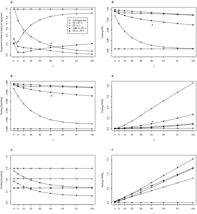
3.1 (a) Expected number of tests per specimen, (b) pooling specificity, (c) pooling sensitivity, (d) poolingP P V, (e) poolingP F ER, and (f) pooling P F ER2 for different algorithms assuming test sensitivity Se = 0.9, test specificity Sp = 0.99, and prevalence p = 0.0002. The N _{denotes the} three stage hierarchical pooling algorithm employed in the NC STAT Program. Note pooling specificity for individual testing equalsSp = 0.99 and is not shown in panel (b). . . 36 3.2 (a) Expected number of tests per specimen, (b) pooling specificity, (c)

pooling sensitivity, (d) poolingP P V, (e) poolingP F ER, and (f) pooling P F ER2 for different algorithms assuming test sensitivity Se = 0.9, test specificitySp = 0.99, and prevalence p= 0.045. TheN_{denotes the three} stage hierarchical pooling algorithm employed in Malawi. . . 37 3.3 (a) Expected number of tests per specimen, (b) pooling specificity, (c)

pooling sensitivity, and (d) pooling P P V for optimally efficient configu-rations ofD3 andA2M assuming test sensitivitySe = 0.9, test specificity Sp = 0.99, and a maximum allowable pool size of 100. . . 38 3.4 Contour plots of (a) expected number of tests per specimen, (b) pooling

sensitivity, and (c) pooling P P V for D3(16 : 4 : 1) assuming p= 0.045 as a function of test sensitivity (Se) and test specificity (Sp). The _• denotes the values of Se and Sp assumed in Table 3.1. . . 39 4.1 Three dimensional planar algorithm (A3P) with L=M =N = 3. The

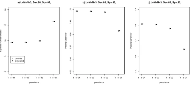
black dots denote 9 (=M N) specimens in one of L planar slices. . . 59 4.2 Results of simulation study. (a) Expected number of tests per specimen,

(b) pooling specificity, (c) pooling sensitivity for A3P assuming L = M = N = 3, test sensitivity Se = 0.88, test specificity Sp = 0.92, and prevalence p_{∈ {}0.0001,0.001,0.01,0.1_}. . . 60 4.3 (a) Expected number of tests per specimen, (b) optimal master pool

size, (c) pooling sensitivity, (d) pooling specificity, (e) poolingP P V and (f) pooling N P V for optimally efficient configurations ofD3,A2M, and A3P M assuming test sensitivity Se = 0.9, test specificity Sp = 0.9, and a maximum allowable pool size of 100. . . 61

5.1 g(q, n) vs. n of A2 for q= (1₋q1 2)

1

4,q = 0.7502, and q = (1− √1

3 2 )

1

(10)

5.3 ∆(q, n) vs. q of A2 forn = 5,6,7,8,9. . . 80

(11)

LIST OF TABLES

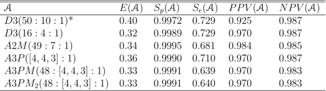
3.1 Comparison of operating characteristics for individual testing and four potential pooling algorithms to be used in Malawi for detection of acute HIV. . . 35

4.1 Description of group testing algorithms. . . 56 4.2 Comparison of operating characteristics for the most efficientD3,A2M,

A3P M, andA3P M2 to be used in NC STAT for detection of acute HIV assuming pool size less than 100, test sensitivitySe = 0.9, test specificity Sp = 0.99, and prevalencep= 0.0002. . . 57

4.3 Comparison of operating characteristics for the most efficientD3,A2M, A3P M, and A3P M2 to be used in Malawi for detection of acute HIV assuming pool size less than 50, test sensitivity Se= 0.9, test specificity Sp = 0.99, and prevalencep= 0.045. . . 58

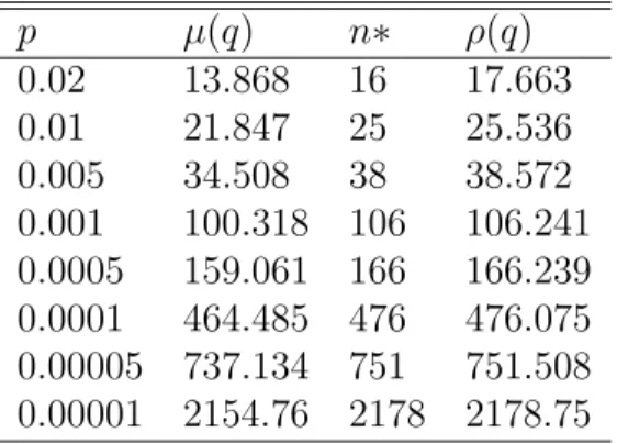
5.1 The behavior of f(q, n) and optimal pool size n_∗ for a given q . . . 81 5.2 Optimal array size n_∗ of A2 for given prevalence p. n_∗ is bounded

(12)

CHAPTER 1 INTRODUCTION

Pooling of specimens to increase efficiency of screening individuals for rare diseases has a long history, dating back to screening for syphilis in military inductees in the 1940s (Dorfman, 1943). Subsequently, specimen pooling orgroup testing has been applied to screening for many other infectious diseases (Quinn et al., 2000; Pilcher et al., 2002; Pilcher et al., 2004; Mine et al., 2003; Kacena et al., 1998; Centers for Disease Control and Prevention, 2003) and has also found broader application in entomology (Venette et al., 2002), screening for genetic mutations (Gastwirth, 2000), the blood bank and pharmaceutical industries (Xie et al., 2001; Jones and Zhigljavsky, 2001), analytical chemistry (Woodbury et al., 1995), information theory (Wolf, 1985) and many other areas.

(13)

Tracing Active Transmission (STAT) program (Pilcher et al., 2002; Pilcher et al., 2005). Likewise, the Center for HIV/AIDS Vaccine Immunology plans to employ similar test-ing procedures as part of a global attempt to identify acute infections (NIAID Office of Communications and Public Liaison, 2005). A similar specimen pooling strategy have also been used to identify acute HIV in antibody negative males attending STD clinics in Malawi.

In these applications, the problem is how to detect very rare cases of HIV infection that elude detection by routine, standard antibody testing assays (Pilcher et al., 2005) because they are in the pre-antibody “acute” phase of infection. The PCR-based nucleic acid amplification assays that detect these persons are highly sensitive but (compared to antibody tests) are expensive, time consuming, and have inadequate specificity (Daar et al., 2001). In this case, group testing is used to enhance testing efficiency and accuracy of high throughput screening for rare cases of acute HIV.

Here we explore aspects of group testing methodology to help optimize the pooling algorithm used in the STAT program and to assist in extending this innovative approach to other settings (e.g. other US states, Africa) or detection of other infectious diseases (e.g., Hepatitis) where the overriding issues are identical but the specific conditions (e.g., disease prevalence) vary considerably.

(14)

of a square-array algorithm in Chapter 5.

(15)

CHAPTER 2 BACKGROUND

2.1 Fundamentals

The pooling of individual serum samples as a cost saving method for diagnosis of infectious disease was first used for identifying individuals with syphilis. The basic idea behind group testing is that for rare diseases, efficiency can be gained by pooling specimens (e.g., urine, sera, or plasma) and testing these pools rather than individual specimens. Here, efficiency is defined in the sense of minimizing the expected number of tests required. A positive test suggests at least one of the specimens in the pool is positive, while a negative test suggests that all specimens in the pool are negative. If the group tests gives a positive result, individual sample is tested. If the group test has a negative result, no more tests are needed. Thus, time and cost can be saved with testing pooled samples rather than individual samples, especially when prevalence rate is very low.

(16)

Pilcher et al., 2005). The recent availability of highly sensitive nucleic acid amplifi-cation tests (NAATs) has created important opportunities for both surveillance and clinical testing of infectious diseases. The possible improvement that NAATs can pro-vide for infectious disease diagnosis is exemplified by HIV. While health authorities have repeatedly emphasized that a goal of HIV testing and surveillance should be to increase detection of early infection, HIV testing has until very recently relied exclu-sively on antibody tests that miss all acute infections, i.e., infections occurring within approximately the last three months during which time individuals are antibody nega-tive and believed to be highly contagious (Pilcher et al., 2004; Wawer et al., 2005). By detecting acute HIV infections and distinguishing them from older infections, NAATs allow for: early treatment of HIV, a strategy which might possibly ameliorate disease pathogenesis; interventions to prevent secondary transmission; better understanding of host-virus dynamics; and improved surveillance (Pilcher et al., 2005).

Unfortunately NAATs are usually considered insufficient for general use due to expense and unacceptably high false positive rates (Pilcher et al., 2002; Klausner, 2004). This lack of specificity results in extremely low positive predictive value in low prevalence settings such as acute HIV. However, NAATs in conjunction with specimen pooling can dramatically improve efficiency, specificity, and positive predictive value (Quinn et al., 2000; Pilcher et al., 2005). For instance, the NC STAT program has now successfully demonstrated that a simple group testing strategy renders NAAT screening much more accurate and cost efficient than testing of individual specimens for acute HIV (Pilcher et al., 2002; Pilcher et al., 2005). This specimen pooling strategy have also been used to identify acute HIV in antibody negative males attending STD clinics in Malawi (Pilcher et al., 2004). Pilcher et al. (2004) concluded that the specimen pooling algorithm has the advantage of being both highly cost efficient and highly specific when used in populations with low expected HIV prevalence.

(17)

2.3 Definitions and Operating Characteristics

In this section, we introduce several definitions and operating characteristics of testing algorithms for case identification in the presence of test error. First, in the group testing problem,stagerefers to the number of sequential steps required by a particular algorithm to identify all positive specimens. In this thesis, we will consider only 2 and 3 stage algorithms.

Define efficiency of a particular pooling algorithm to be the expected number of tests per specimen required to identify all positive specimens. For a group testing algorithm A_{, denote the efficiency by}_E(A_).

Define pooling specificity to be the probability an individual is categorized as neg-ative by a particular pooling procedure given that individual is truly negneg-ative (Litvak et al. 1994; Johnson et al. 1991). Similarly, define the pooling sensitivity to be the probability an individual is categorized as positive by a particular pooling procedure given that individual is truly positive. Denote the pooling specificity and sensitivity for

A _by _Sp(A_{) and} _Se(A_{). For example, if} I _{denotes individual testing, then} _Sp(I_{) =} _Sp and Se(I_{) =}_Se.

Define thepooling positive predictive valueofA_{to be the probability an individual is} truly positive given they are categorized as positive byA_{. Likewise, define the} _pooling negative predictive value of A _{to be the probability an individual is truly negative} given they are categorized as negative byA_{. Denote the pooling positive and negative} predictive values of A _by _{P P V}₍A_{) and} _{N P V}₍A_{). The predictive values are simple} functions ofSe(A_{) and}_Sp(A_):

P P V(A_{) =} pSe(A)

(18)

and

N P V(A_{) =} qSp(A)

p[1₋Se(A_{)] +}_qSp(A₎.

Additionally, we consider other error rates that have been proposed in the multiple comparisons literature (Cook and Dunnett, 1998), but to our knowledge have not been considered in the context of group testing. These quantities provide alternative metrics for quantifying the degree of misclassification of negative individuals as positive and positive individuals as negative.

Define theper-family error rate(P F ER) to be the expected number of false positive classifications and the per-comparison error rate (P CER) to be the expected number of false positive classifications divided by the total number of specimens (Hochberg and Tamhane, 1987). In Appendix A, we show that P F ER(A_{) =} _nq_{₁₋ _Sp(A₎_} for any pooling algorithm A_{, which immediately gives} _{P CER(}A_{) since} _{P F ER(}A_{) =} nP CER(A_{) where}_n _{is the number of specimen to be tested.}

Define the type II per-family error rate (P F ER2) to be the expected number of false negative classifications and thetype II per-comparison error rate(P CER2) to be the expected number of false negative classifications divided by the total number of specimens. In Appendix A, we also show that P F ER2(A_{) =} _np_{₁₋_Se(A₎_} _{for any} pooling algorithmA_{, which gives} _{P CER2(}A_{) since}_{P F ER2}₍A_{) =} _{nP CER2(}A_).

2.4 Dorfman Algorithm

Dorfman (1943) studied the application of a group testing procedure for screening men called up for induction into the army for presence of syphilitic antigen. Case identification (or classification) was the original motivation behind group testing, as proposed by Dorfman (1943). Dorfman’s algorithm entailed pooling together biological specimens from several individuals and testing these pools of specimens rather than

(19)

testing each individual specimen. If a pool tested negative, all specimens in that pool were declared negative. Otherwise, further testing on individual specimen from the pool were employed to identify all positive individuals.

He derived the expected number of tests which is equal to one master pool plus the number of individuals in the master pool which require individual testing. Using notation from the Section 2.3, it is easy to see that the expected number of tests per specimen is

E

T n

= 1

n + 1−q

n_, _(2.1)

where T is the number of tests and n is the pool size. Dorfman’s original pooling algorithm required simply testing all individual specimens within positive master pool without considering classification errors. This pooling procedure is appealing in that, for rare diseases, fewer number of tests are required on average to identify all cases compared to individual testing. His method was applied to blood tests for syphilis and found optimal group sizes, which minimize the expected number of tests per specimen, for various fixed values of p and concluded that his method is more efficient when compared to individual testing, for small values of p ranging from .01 to .15. Note that optimal size n= √1_p of Dorfman’s procedure was obtained by Feller (1957), Wilks

(1962), Samuels (1978) and Turner et al. (1988).

(20)

rather than perform individual testing as both Dorfman and Sterrett procedures advo-cate. If the subgroup tests positive, the remaining samples from the original positive group are treated as if they were never tested. This is statistically accurate so long as the population of items being tested is binomial. If the subgroup tests negative, it is completely classified, and a new subgroup is drawn from the remaining members of the original group. Sobel and Groll (1959)’s procedure is complicated since optimal group (subgroup) sizes have to be determined at each stage of testing. Also, in its worst case, it can require a very large number of tests to classify the entire population. Hwang (1972) moved away from the assumption that the number of defectives is binomial and developed a procedure based on an upper bound for the number of defectives or its probability distribution. Johnson et al. (1991) generalized Dorfman’s pooling algo-rithm in the presence of test error and extended to hierarchical algoalgo-rithm. Lancaster and Keller-McNulty (1998) and Venette et al. (2002) reviewed sampling method and analyzed generalizations of Dorfman’s pooling algorithm.

2.5 Hierarchical Algorithms

A simple extension of Dorfman’s original procedure entails repeatedly dividing positive pools into smaller, non-overlapping subpools until eventually all positive specimens are individually tested. We refer to this approach as ahierarchical group testing algorithm (Finucan, 1964; Johnson et al., 1991; Litvak et al., 1994). For example, the NC STAT program (Pilcher et al., 2002) employs a three stage hierarchical algorithm as follows. First, disjoint master pools of 90 specimens are tested. Second, positive master pools are divided into subpools of 10 specimens each and these subpools are tested. Third, specimens from positive subpools are individually tested. Similar hierarchical pooling algorithms have been used for the detection of recent HIV infections in Malawi (Pilcher

(21)

et al., 2004) and India (Quinn et al., 2000).

Johnson et al. (1991) considered hierarchical group testing algorithms in the pres-ence of test errors. They derived the expected number of tests, pooling sensitivity and pooling specificity for a hierarchical algorithm. They also allow sensitivity and specificity to be dependent on the number of pool size of each stage.

Litvak et al. (1994) generalized some commonly used pooling procedures. They presented group testing methods in which positive groups are split into several sub-groups of almost equal size. Any subsub-groups that test positive are further split into even smaller subgroups and this process continues until items are tested individually. They called this method T2 and extended it as T2+. T2+ is same as T2 except that

each group that produces a negative outcome is retested at mostr₋1 times where ris the maximum number of times a group will be retested before being classified or split further into smaller groups. If all r₋1 tests are negative, the group is classified as negative (r = 2 in Litvak et al. (1994)). Otherwise, it is classified as positive. Litvak et al. (1994) compared several such procedures with each other and with Dorfman’s procedure for different values of test reliability. They concluded that T2 and T2+ are

better than Dorfman’s procedure. They also concluded that if the purpose of screening is to determine the infectious status of individuals and estimate prevalence, thenT2 is

more competitive in this screening situation. However, if the goal is to screen donated blood,T2+ should be chosen, since this is the only procedure that reduces theF N P V.

(22)

2.6 Square Array Algorithms

Array based specimen pooling is an alternative to hierarchical group testing which

uses overlapping pools. While the corresponding pooling algorithms are more complex,

array based group testing can be very efficient. This approach is frequently employed

in genetics (Bruno et al., 1995; Amemiya et al., 1992; Barillot et al., 1991; Zwaal et al.,

1993), but remains largely underutilized in the infectious disease setting. In its simplest

form, n2 specimens are placed on an n_×n matrix. Pools of size n are made from all samples in the same row or in the same column. These 2n pools are then tested and,

assuming no false negative tests, all positive specimens will lie at the intersection of a

positive row pool and a positive column pool. Any ambiguities are resolved by testing

all specimens at these intersections.

Phatarfod and Sudbury (1994) evaluated the use of a two-dimensional array scheme.

Their idea was based on the observation that blood samples are often placed in a square

tray, and one could exploit this arrangement by compositing across rows and columns.

Tests were conducted on the row and column composite samples, and confirmatory

tests were conducted on sample units at the intersection of positive row and column.

They called this scheme asSA1 and derived the expected number of tests per specimen:

E(SA1) = _n2 + 1₋2qn₊_q2n−1_. _(2.2)

A second scheme,SA2 which was proposed by Phatarfod and Sudbury (1994), proceeds as forSA1 expect that if all rows test negative no further tests are done (ntests in all), and if exactly one row tests positive then each individual in that row is tested (2n tests

in all). WhileSA2 requires one more stage than SA1, Phatarfod and Sudbury (1994) showedSA2 requires fewer tests thanSA1 and the Dorfman scheme forpranging from .000001 to .05. Phatarfod and Sudbury (1994) also considered rectangularm_×narray

(23)

schemes, e.g., the classical 8_×12 array and concluded that these schemes also require fewer tests than the Dorfman scheme.

Woodbury et al. (1995) noted that testing row and column pools, without further testing, results in ambiguities in assigning true sample locations. In order to resolve these ambiguities, they proposed pooling samples along diagonals of the array, wherein the diagonals are wrapped around the array so that each diagonal pool contains the same number of samples as each row and column pool.

Unfortunately, there are limitations in directly applying the array based procedures proposed in the literature to the infectious disease setting. For example, several pro-posed array pooling algorithms do not guarantee that all cases will be unambiguously identified (Woodbury et al., 1995; Bruno et al., 1995). For instance, diagonal pooling as suggested by Woodbury et al. (1995) will not resolve all ambiguities if all specimens in the first row and first column are positive. Perhaps most importantly, with the exception of Section 5 of Phatarfod and Sudbury (1994), the array based group testing literature does not consider test error, i.e., false positive and false negative test results.

2.7 Multidimensional Array Algorithms

Berger et al. (2000) extended Phatarfod and Sudbury (1994) to higher dimensional arrays. They proposed two natural three-dimensional extensions of the basic matrix method to an L_×M _×N cubic array, the three-dimensional planar method and the three-dimensional linear method.

For the three-dimensional planar method (called 3P), in stage 1, each of the L

planar slices from front to back, the M planar slices from top to bottom, and the N

(24)

The efficiency of the 3P method is the sum of four terms, namely, the reciprocals of LM, LN, M N and the quantity (1₋qLM ₋_qLN ₋_qM N ₊_qL(M+N−1)₊_qM(L+N−1) ₊ qN(L+M−1)₋_qLM+LN+M N−L−M−N+1_{). For example, if}_L ₌_M ₌_{N, then the expected} number of tests per specimen of algorithm 3P equals

3

N2 + 1−3qN 2

+ 3qN(2N−1) ₋_q3N2₋_3N+1

. (2.3)

For the three-dimensional linear method (called 3L), in stage 1, for each of theM N sites on the front face of the cube, test the group of size L on the line perpendicular to this face through this site. Repeat for the LN groups of size M lying on similar lines perpendicular to the top and the bottom faces and for the LM groups of size N located on lines perpendicular to the left and right faces. In stage 2, test individually each specimen located at the intersections of three lines that all tested positive in stage 1. They showed the extension of 3L to multiple dimensions, denoted by M L, yields the family of maximally efficient positive testing procedures and the most efficient multidimensional parallelepiped is a generalized cube. Berger et al. (2000) proved that the efficiency of M Lfor a d- dimensional cube whose side have length s is

ds−1 ₊_p₊_q(1₋_qs−1₎d_. _(2.4)

The optimal procedures proposed by Berger et al. (2000) are not necessarily clinically feasible due to the requirement of extremely large numbers of specimens. For example, the parameters s = 74 and d = 6 that maximize efficiency when p = .01 require sd_{= 74}6 _≈_{164 billion items to be in the population to be screened.}

Schuster (2002) indicated there exists a theoretical connection between the work of Berger et al. (2000) and design theory. Design theory is the study of combinatorial design, which is an arrangement of the elements of a finite set into subsets or arrays

(25)

which satisfy certain regularity conditions. For example, thirty-six officers are given, belonging to six regiments and holding six ranks. One wants to know that the officers can be paraded in a 6_×6 array so that, in any line (row or column) of the array, each regiment and each rank occurs exactly once. Design theory deals with this kind of problem of arranging objects according to certain rules. Schuster (2002) showed how design theory can be employed to determine optimal array algorithms which require much smaller numbers of specimen than reported in Berger et al. (2000).

Roederer and Koup (2003) used various multidimensional array pooling algorithms to identify T cell immune responses to vaccines or pathogens and used a Monte Carlo simulation to optimize the construction of peptide pools that could identify responses to individual peptide using the fewest numbers of assays and patient material. They found that the number of assays required to deconvolute a pool increases by the logarithm of the number of peptides within the pool. However, the optimum configuration of pools changes dramatically according to the number of responses to individual peptides that are expected to be in the sample.

2.8 Error Rates

A majority of the group testing literature assumes testing is done without error, i.e., assumes 100% sensitivity and specificity. For instance, Dorfman (1943) does not con-sider classification errors. Phatarfod and Sudbury (1994) developed two dimensional array methods without test errors except briefly in Section 5.

(26)

specificity to depend on pool size.

Litvak et al. (1994) focused on HIV antibody tests and considered sensitivity and specificity as inherent characteristics of the test kit that influence how accurately an individual sample can be classified. They assumed the underlying test kits all have the same sensitivity and the same specificity at each step of the testing and for all samples. High incidence of false positives is commonly reported in HIV antibody screening of blood samples. Litvak et al. (1994) calculated that when prevalence rate is 4 per 10,000 people and a test kit having a sensitivity and a specificity of 98% is used, the false positive predictive value of test can be as high as 0.98.

Wein and Zenios (1996) attempted to capture the dilution effects. Adilution effects is defined as the failure of the test to detect an infected sample when it is mixed with a large number of negative samples. They developed a generalized linear model which connects optical density or OD levels (the attribute that is observed and measured in an ELISA test) with the antibody concentration in the pooled serum and later used it in a dynamic programming algorithm to produce a testing strategy which minimizes the total expected cost. Total cost is the sum of testing cost and the cost of incorrect classifications. It should be noted that, unlike others, these authors allowed three possibilities at each stage of testing: declare the group negative; require further testing, and declare all members of the group positive.

Gupta and Malina (1999) modified Dorfman and Sterrett’s group testing protocols in the presence of classification errors. They begin with a highly sensitive test to achieve virtually 100% sensitivity. Specimens are tested in groups and individually as prescribed by the modified Dorfman and Sterrett methods. They controlled the incidence of false positives by repeating tests of grouped and individual samples that are initially reactive. The number of retests is chosen carefully so as to bring the overall incidence of false positives below some desired level, usually set close to 0. They

(27)

also compared the modified Dorfman and the modified Sterrett procedures with their

modified individual testing and showed that the modified Dorfman and the modified

Sterrett are more efficient than the modified individual testing in the presence of test

errors and the modified Sterrett is slightly efficient than the modified Dorfman, but

harder to implement.

2.9 Optimal Pool Size

Feller (1957) and Wilks (1962) have presented text-book exercises which showed the

optimal pool size,n = _√1

p of Dorfman algorithm. Finucan (1964) gave an approximation

to the optimal hierarchical scheme when there exist no test errors. Samuels (1978)

provided a simple method to obtain the optimal pool size for the Dorfman algorithm

without test errors, while correctly indicating the fault of the assumption of unimodality

used by Finucan and others. Turner et al. (1988) mentioned neither Wilks’ method

nor Feller’s approximation always lead to the optimal pool size. They used a calculus

based approach and Wilks’ suggestion to get the optimal pool size. Wu and Zhao (1994)

provided a concrete procedure to determine the precise optimal plan which minimizes

the expected number of tests per specimen for hierarchical group testing problem when

(28)

CHAPTER 3 HIERARCHICAL AND SQUARE

ARRAY ALGORITHMS

3.1 Introduction

The focus of this chapter is to research the utility of two-dimensional array-based group

testing algorithms for case identification in the presence of test error.

Array-based specimen pooling is an alternative to hierarchical group testing which

uses overlapping pools. In its simplest form, n2 _{specimens are placed on an} _n_× _n matrix. Pools of size n are made from all samples in the same row or in the same column. These 2n pools are then tested and, assuming no false negative tests, all positive specimens will lie at the intersection of a positive row pool and a positive

column pool. Any ambiguities are resolved by individually testing all specimens at

these intersections. Phatarfod and Sudbury (1994) derived the expected number of

tests for two-dimensional array (i.e., matrix) group testing procedures. This approach

is also employed in genetics (Bruno et al. 1995; Amemiya et al. 1992; Barillot, Lacroix,

and Cohen 1991) . However, with the exception of Section 5 of Phatarfod and Sudbury

(29)

In this chapter, we derive and compare the operating characteristics of hierarchical

and square array based testing algorithms for case identification in the presence of

testing error. We assume constant sensitivity and specificity for each test independent

of pool size for this chapter. The operating characteristics investigated include efficiency

(i.e., expected number of tests per specimen) and error rates (i.e., sensitivity, specificity,

positive and negative predictive values, per-family error rate, and per-comparison error

rate). The methodology is illustrated by comparing different pooling algorithms for the

detection of individuals recently infected with HIV in North Carolina and Malawi.

3.2 Assumptions

In order to derive operating characteristics of the various pooling algorithms considered,

we make the assumptions enumerated below. These assumptions are general enough

to apply to both the hierarchical and square array algorithms.

Assumption 1 All specimens are independent and identically distributed with proba-bility p of being positive.

We refer to p as the prevalence and letq = 1₋p.

Assumption 2 Given a pool P _{containing at least one positive specimen is tested, the} probability P _{tests positive equals} _S_e.

We refer to Se as thetest sensitivity. Assumption 2 implies that the test sensitivity is independent of the number of specimens within a pool and the number of positive

specimens therein. It follows that Se is also the sensitivity for a test of an individual

specimen, i.e., a pool of size 1. We do not consider here more elaborate models where

test sensitivity depends on the number of specimens within a pool, i.e., dilution effects

(30)

that the results in this paper are applicable only to settings where the largest pool size

is not believed to suffer appreciable dilution effects. Determination of the maximum

allowable pool size will be application specific. For example, Litvak et al. (1994)

consider pool sizes up to 15 specimens when using an ELISA test to detect individuals

with HIV antibodies. Another example is given by detection of acute HIV in antibody

negative populations where NAATs are thought to be sufficiently sensitive such that

pools of size 90 or 100 are often used in practice (Quinn et al., 2000; Pilcher et al.,

2002; Pilcher et al., 2005).

Assumption 3 Given a pool P _{containing no positive specimens is tested, the} proba-bility P _{tests positive equals} ₁₋_S_p_.

We refer to Sp as the test specificity. Assumption 3 implies test specificity is inde-pendent of pool size.

3.3 Hierarchical Algorithm

In this section, we present the efficiency and error rates of a hierarchical group testing

algorithm withS stages under Assumption 1-3. These results first appeared in Johnson

et al. (1991), but often go unrecognized in the literature and thus are restated here.

Consider a hierarchical algorithm where a master pool of size n1 = k1k2· · ·kS−1 is tested at first stage where k1k2 · · · kS−1 are positive integers. If the master pool tests positive, then k1 pools of size n2 =k2 · · ·kS−1 are tested, and so forth. Denote this algorithm by A ₌ _DS₍_n₁ _: _n₂ _: _n₃ _: _{. . .} _: _n_S

−1 : nS) where n1 = k1k2 · · ·kS−1,

n2 = k2 · · ·kS−1, · · ·, nS−1 = kS−1, nS = 1. Let Xsi be random variables that equal 1 if the ith _{pool in} _sth _stage _tests _{positive, and 0 otherwise for} _s _{= 1}_{, . . . , S} _and

i= 1, . . . , n1/ns.

(31)

3.3.1 Efficiency

Let the number of tests be T = T1 +T2 +T3 +. . .+TS where Ts is the number of

tests at thesth _{stage for}_s_{= 1}_,₂_,₃_{, . . . , S}_{. Then the expected number of tests given} _n 1

specimens equals

E(T) = 1 +k1E(X1i) +k1k2E(X2i) +. . .+n1E(XS−1,i).

From equation (6.18) of Johnson et al. (1991),

E(Xsi) =qn1(1−Sp)s+Psj=1−1(qnj+1−qnj)Sej(1−Sp)s−j+ (1−qns)Ses, (3.1)

for s= 1,2, . . . , S₋1.

From equation (3.1), it follows that for a two-stage hierarchical algorithm, i.e.,

S = 2, the expected number of tests per specimen forD2 is

E(D2)_≡E

T n1

= 1

n1

+f(n1), (3.2)

where f(n)_≡(1₋Sp)qn₊_S_e(1₋_qn_{), is the probability a pool of size} _n _{tests positive}

without any knowledge of the true status of the pool. For notational simplicity, we

suppress the dependence of f on the parameters p, Se, and Sp. For given values of p,

Se, and Sp, the optimally efficient two stage procedure is determined by the value of n

that minimizes (3.2). Special cases of (3.2) were also derived by Litvak et al. (1994)

and Gastwirth (2000). In particular, for n1 = 15, (3.2) reduces to the first equation in

Section 2.4 of Litvak et al. (1994). Similarly, ifSe = 1, (3.2) reduces to equation (2) of

Gastwirth (2000).

(32)

that the expected number of tests per specimen for D3 is

E(D3)_≡E

T n1

= 1

n1 + f(n1)

k2 +Se 2₍₁

−qk2_{) + (1}₋_S

p)f(n1−k2)qk2. (3.3)

Finucan (1964) showed that, in the absence of test error,n2 =√n1 is approximately

optimal with regards to minimizing the expected number of tests per specimen. Thus

in the Application below (Section 3.7) we primarily consider configurations ofD3 where

n2 =√n1.

3.3.2 Error rates

From equations (6.15) and (6.16) of Johnson et al. (1991), the pooling sensitivity and

specificity ofDS are

Se(DS) =SeS, (3.4)

and

Sp(DS) = 1−PSs=1(qns−1−qns−1−1)Ses−1(1−Sp)S−(s−1), (3.5)

where qn0−1 _≡_{0. It follows that the pooling sensitivity and specificity of the Dorfman}

procedure (i.e.,S = 2) are

Se(D2) =Se2, (3.6)

and

Sp(D2) = 1−(1−Sp)f(n1−1). (3.7)

For n1 = 15, (3.6) and (3.7) reduce to equations (1) and (4) of Litvak et al. (1994).

For S = 3, the pooling sensitivity and specificity are Se(D3) = Se3, and Sp(D3) =

1₋[(1₋Sp){(1−Sp)f(n1−k2)qk2−1 +Se2(1−qk2−1)}]. Note because Se3 ≤ Se2 ≤ Se, neitherD2 nor D3 will ever improve over individual testing in terms of sensitivity.

(33)

3.4 Square Array without Master Pool Testing

In this section, we derive the operating characteristics of a two-stage square array

testing algorithm in the presence of testing error, denoted by A2(n: 1). In particular,

consider the n _×n square array set-up of Phatarfod and Sudbury (1994) where n2

specimen are placed on an n _×n matrix. Pools are then made from all samples in

the same row or in the same column. These 2n pools (n row pools and n column

pools) are then tested and, assuming no test error, all positive specimens will lie at the

intersection of a positive row pool and a positive column pool. Therefore all specimens

at the intersection of a positive row and a positive column are subsequently tested.

However, when there is testing error, one must allow for the possibility of positive row

pools and no positive column pools (or vice-versa). Thus we assume that the (i, j)th sample is tested individually if either both theith _{row and the}_jth _{column test positive,} the ith _{row tests positive but all columns test negative, or the}_jth _{column tests positive} but all rows test negative. Let Ri represent the test outcome of the ith _{row, and} _Cj represent the test outcome of the jth _{column. Similarly, denote the true values by} _RT i and CT

j . Let Xij denote the test outcome of individual (i, j) and Yij denote the true status of individual (i, j) such that RT

i = I[ P

jYij > 0] and CjT = I[ P

iYij > 0]. We will make the following additional assumption to derive efficiencies and error rates for

array pooling algorithms:

Assumption 4 Given the true status of ith _{row and} _jth _{column, the} _ith _{row and} _jth column tests are conditionally independent of each other.

3.4.1 Efficiency

Let the number of tests be T = T1 +T2, where T1 = 2n corresponds to the row and

(34)

testing where

T2ij =                 

1 if Ri = 1 andCj = 1

1 if Ri = 1 and P

Cj = 0

1 if P

Ri = 0 andCj = 1

0 otherwise

. (3.8)

To derive the expected number of tests, by symmetry we write

E(T2ij) = Pr[Ri = 1, Cj = 1] + 2 Pr[Ri = 1,X

j

Cj = 0]. (3.9)

The first component of the right side of (3.9) equals

Pr[Ri = 1, Cj = 1] =P1_r,c=0Pr[Ri = 1, Cj = 1_|RT

i =r, CjT =c] Pr[RTi =r, CjT =c].

Under Assumptions 1 - 4, direct substitution and some algebra yields

Pr[Ri = 1, Cj = 1] = (1₋Sp)2_q2n−1_{+ 2}_Se₍₁₋_Sp₎₍₁₋_qn−1₎_qn₊_S2

e(1−2qn+q2n−1)

=Sef(n) + (1₋Sp₋Se)qn_f₍_n₋₁₎_≡_g₍_n₎_.

The second component of the right side of (3.9) can be written as

1 X r=0 n X c=0

Pr[Ri = 1,X

j

Cj = 0_|R_iT =r,X j

C_jT =c] Pr[RT_i =r,X

j

C_jT =c]. (3.10)

Forc_{∈ {}0, . . . , n_}, let

β0(c)_≡Pr[R_iT = 0,X j

C_jT =c] =

n

c

(qn2−cn+c)(1₋qn−1)c, (3.11)

β1(c)_≡Pr[RT_i = 1,X j

C_jT =c] =

n c

qn2−cn(1₋qn)c₋β0(c), (3.12)

(35)

γ0(c)≡Pr[Ri = 1,

X

j

Cj = 0|RTi = 0,

X

j

C_jT =c] = (1₋Sp)(1−Se)cSpn−c,

and

γ1(c)≡Pr[Ri = 1,

X

j

Cj = 0|RiT = 1,

X

j

C_jT =c] =SeSpn−c(1−Se)c,

where we define γ1(0) ≡0. Then it follows that

Pr[Ri = 1,

X

j

Cj = 0] = n

X

c=0

{γ0(c)β0(c) +γ1(c)β1(c)} ≡h(n),

such that the expected number of tests per specimen forA2 is

E(A2)_≡E

T n2

= 2

n +g(n) + 2h(n). (3.13)

Note if Se = Sp = 1, then h(n) = 0, g(n) = f(n)−qnf(n −1) and f(n) = 1−qn

such thatE(A2) = 2/n+ 1₋2qn₊_q2n−1_{, which equals equation (2) of Phatarfod and}

Sudbury (1994).

3.4.2 Error rates

Fori_{∈ {}1, . . . , n_}and j _{∈ {}1, . . . , n_},

1₋Sp(A2) = Pr[Xij = 1|Yij = 0]

= Pr[Ri = 1, Cj = 1, Xij = 1|Yij = 0] + 2 Pr[Ri = 1,PkCk = 0, Xij = 1|Yij = 0]

= Pr[Xij = 1|Yij = 0, Ri = 1, Cj = 1] Pr[Ri = 1|Yij = 0] Pr[Cj = 1|Yij = 0]

+2 Pr[Xij = 1|Yij = 0, Ri = 1,PkCk= 0] Pr[Ri = 1,PkCk = 0|Yij = 0]

= (1₋Sp)f(n−1)2+ 2(1−Sp) Pr[Ri = 1,PkCk = 0|Yij = 0],

(3.14)

where the second equality is from the definition of algorithmA2 given by (3.8) and the

(36)

0] =f(n₋1). Next let

h(n_|y) _≡Pr[Ri = 1,P_kCk= 0|Yij = 0]

=P1

r=0

Pn

c=0

Pr[Ri = 1,P_kCk = 0|RTi =r,

P

kCkT =c, Yij = 0]

×Pr[RT i =r,

P

kCkT =c|Yij = 0] ,

(3.15)

β0(c|y) ≡Pr[RTi = 0,

P

kCkT =c|Yij = 0] = β0_q(c),

and

β1(c|y) ≡Pr[RiT = 1,

P

kCkT =c|Yij = 0] = Pr[P_kCkT =c|Yij = 0]−β0(c|y)

= n−_c1

(1₋qn₎c_qn2₋_nc₋₁

+ n_c₋−₁1

(1₋qn₎c−1_qn2₋_nc

(1₋qn−1₎₋_β 0(c|y),

for c_{∈ {}0, ..., n_}where β1(0|y)≡0. Then

h(n_|y) =

1 X r=0 n X c=0

βr(c|y)γr(c), (3.16)

since γr(c) ≡ Pr[Ri = 1,PkCk = 0|RTi = r,

P

kCkT = c, Yij = 0]. Thus, (3.14) is

equivalent to

Sp(A2) = 1− {(1−Sp)f(n−1)2+ 2(1−Sp)h(n|y)}. (3.17)

We can derive pooling sensitivity using several applications of Assumptions 1 and

2:

(37)

Se(A2) = Pr[Xij = 1|Yij = 1]

= Pr[Ri = 1, Cj = 1, Xij = 1|Yij = 1] + 2 Pr[Ri = 1,PkCk= 0, Xij = 1|Yij = 1]

=S3

e + 2Se2Pr[Cj = 0|Yij = 1]Q_k₆_=jPr[Ck = 0]

=S3

e + 2Se2(1−Se) Pr[Ck = 0]n−1

=S3

e + 2Se2(1−Se){1−f(n)}n−1.

(3.18)

3.5 Square Array with Master Pool Testing

We also consider a three-stage square array testing where we first test a master pool

of size n2_{. If the master pool tests negative, the procedure stops. Otherwise, the}

procedure continues as inA2. Denote this square array testing procedure with master

pool testing by A2M(n2 _:_n_{: 1).}

3.5.1 Efficiency

Let the number of tests be T =T0+T1+T2 where T0 = 1 corresponds to testing the

master pool, T1 corresponds to possible row and column testing and T2 corresponds

to possible individual testing. To compute the efficiency of A2M, let X0 be a random

variable that equals 1 if the master pool tests positive and 0 otherwise such thatT1 =

2nX0 and E(T1) = 2nf(n2). Next write T2 =Pi,jT2ij where

T2ij = 

       

       

1 if X0 = 1, Ri = 1 andCj = 1

1 if X0 = 1, Ri = 1 and PCj = 0

1 if X0 = 1,PRi = 0 andCj = 1

(38)

such that the expected number of tests per specimen for A2M is E(A2M) _≡ _n12 +

2 nf(n

2_{) +}_E_(T2ij_{), where}

E(T2ij) = Pr[X0 = 1, Ri = 1, Cj = 1] + 2 Pr[X0 = 1, Ri = 1,X j

Cj = 0]. (3.19)

It is straightforward to show the first part of the right side of (3.19) equals

Pr[X0 = 1, Ri = 1, Cj = 1] = (1₋Sp)2_qn2

(1₋Sp ₋Se) +Seg(n). (3.20)

Likewise, the second part of the right side of (3.19), i.e., Pr[X0 = 1, Ri = 1,P

jCj =

0], can be written as

P1

r=0

Pn

c=0

n

Pr[Ri = 1,P

jCj = 0|X0 = 1, RTi =r,

P

jCjT =c]

×Pr[X0 = 1|RTi =r,

P

jCjT =c] Pr[RTi =r,

P

jCjT =c]

o

,

which implies

Pr[X0 = 1, Ri = 1,P

jCj = 0] = (1−Sp)γ0(0)β0(0) +Se

Pn

c=1{γ0(c)β0(c) +γ1(c)β1(c)_} = (1₋Sp₋Se)γ0(0)β0(0) +Seh(n).

Therefore the expected number of tests per specimen for A2M is

E(A2M) = 1

n2 + (1−Sp−Se)q n22

n + (1−Sp)

2_{+ 2(1}

−Sp)S_pn

+SeE(A2).

(39)

3.5.2 Error rates

To derive the pooling specificity of A2M, write

1₋Sp(A2M) = Pr[Xij = 1|Yij = 0]

= (1₋Sp)µ(n|y) + 2(1−Sp)ν(n|y)

(3.21)

where

µ(n_|y) = Pr[X0 = 1, Ri = 1, Cj = 1|Yij = 0]

=f(n2₋_2n_{+ 1)}_{₍₁₋_Sp)qn−1_}2₊_S2

e(1−qn−1){(1−Sp)qn−1+f(n−1)},

and

ν(n_|y) = Pr[X0 = 1, Ri = 1,PkCk= 0|Yij = 0]

= (1₋Sp)β0(0|y)γ0(0) +SeP1r=0

Pn

c=1βr(c|y)γr(c),

since γr(c) = Pr[Ri = 1,P

kCk = 0|RiT =r, P

kCkT =c, Yij = 0, X0 = 1].

Applying Assumptions 1 and 2 several times, pooling sensitivity equals

Se(A2M) = Pr[Xij = 1, Ri = 1, Cj = 1, X0 = 1|Yij = 1]

+2 Pr[Xij = 1, Ri = 1,PkCk= 0, X0 = 1|Yij = 1]

=S4

e + 2Se3(1−Se){1−f(n)}n−1.

(3.22)

3.6 Assessing Variability

Thus far we have presented expressions for different group testing algorithm

parame-ters such as the expected number of tests, pooling sensitivity and pooling specificity.

Formulae for pooling predictive values (P P V and N P V) and the other error rates

de-scribed in Section 2.3 follow immediately. However, for a particular set of specimens,

theobserved number of tests may differ from the expected number of tests due to

(40)

observable in the absence of a gold standard test, clearly these latent “observed” error

rates may also differ from the corresponding parameter values due to sampling

variabil-ity. Quantifying this uncertainty associated with the different operating characteristics

can be helpful in comparing different pooling strategies. For example, if two group

testing procedures have comparable expected number of tests, the one with smaller

variance may be preferable operationally.

Explicit expressions for the variance associated with the number of tests per

speci-men for D2, D3, A2, and A2M are derived in the Appendix B. In turn, large sample

probability intervals (PIs) for the observed number of tests per specimen can be

com-puted by appealing to the Central Limit Theorem. For instance, suppose N samples

are to be tested using D3(n : √n : 1) with N sufficiently larger than n. Then there

is an approximate (1₋α) probability that the observed number of tests per specimen

required to identify allN individuals as positive or negative will be in the PI

E(D3)_±z1₋α/2

s

V ar(D3)

N/n ,

wherez1₋α/2 is the 1−α/2 quantile of the standard normal distribution, E(D3) is given

by equation (3.3) and V ar(D3) follows from equation (B.2) in Appendix B.2. Similar

reasoning can be employed to obtain PIs for the observed number of tests using D2,

A2, and A2M.

The cumulative distribution functions (CDFs) for the observed pooling sensitivity,

specificity, and predictive values are derived in Appendix C. Using these CDFs,

cor-responding PIs can easily be determined. For instance, we show that for any pooling

algorithm A _{applied to} _N _{specimens, the CDF of the observed sensitivity (}_SO e (A))

(41)

equals

Pr[S_eO(A₎_≤_{s] =}

N

X

y=0 bsyc

X

x=0

y x

Se(A)x(1−Se(A))y−x

N

y

py(1₋p)N−y,

where _bsy_c denotes the largest integer less than or equal to sy. Using this expression,

an approximate (1₋α) PI for the observed sensitivity is given by (sL, sU) wheresL is

the largest value such that Pr[SO

e (A) ≤ sL] ≤ α/2 and sU is the smallest value such

that Pr[SO

e(A) ≥ sU] ≤ α/2. PIs for pooling specificity and predictive values follow

analogously using the corresponding CDFs given in Appendix C.

3.7 Application

Using the results derived above, in this section we explore the operating characteristics

of individual testing, D2, D3, A2, and A2M for identification of acute HIV using

NAATs. For our first example, we consider a setting similar to the NC STAT program.

First, we assume prevalence of acute HIV is p = 0.0002 (Pilcher et al., 2005) and

NAAT has a 99% test specificity (Hecht et al., 2002) and 90% test sensitivity. Suppose

further we are limited to a master pool size of 100 due to dilution effects (Quinn et al.,

2000). Under these assumptions, Figure 3.1 depicts the efficiency, pooling sensitivity,

specificity, P P V and P F ERs of individual testing, D2(n : 1), D3(n : √n : 1) (here

k2 =√n),A2M(n :√n : 1), and A2(√n: 1) as a function of the number of specimens

n. (Recall that D2(n : 1) denotes two-stage hierarchical testing with pools of size n

in the first stage; D3(n:√n : 1) denotes three-stage hierarchical testing with pools of

size n at the first stage and pools of size √n at the second stage; A2(√n : 1) denotes

two-stage √n_×√n array testing; and A2M(n :√n: 1) denotes three-stage √n_×√n

array testing wherein the first stage entails testing a master pool of sizen.) The panel

(42)

n= 100. The expected number of tests per specimen for D3(90 : 10 : 1), the algorithm

currently employed by the NC STAT program, is 0.016. ForN = 8,505 total specimens

(Pilcher et al., 2002), the 95% PI for efficiency ofD3(90 : 10 : 1) is (0.010, 0.021), which

contains the observed rate of 0.018 reported by Pilcher et al. (2002). Under these same

conditions, the expected number of tests per specimen is also 0.016 (95% PI: 0.008 to

0.024) for A2M(100 : 10 : 1). Panels (b) and (d) of Figure 3.1 indicate D3 and A2M

are also preferable with regards to pooling specificity and, especially, P P V. However

these two algorithms are also the least sensitive as depicted in panel (c) of Figure 3.1.

Panel (e) of Figure 3.1 indicates D3 and A2M are preferable with regards to pooling

P F ER. We also see that other algorithms are better than individual testing with

regards to the efficiency, pooling specificity, P P V and P F ER. Overall, these results

suggest by moving from D3(90 : 10 : 1) to A2M(100 : 10 : 1), could improve pooling

specificity, sensitivity, P P V, P CERs, and P F ERs without sacrificing efficiency. In

particular, given the NC STAT program processes 120,000 specimens per year, this

change in pooling algorithm would result in a decrease in P F ER2 from 6.5 to 5.1. In

other words, on average 1-2 additional acute HIV cases would be detected each year,

representing a 5-10% increase over the current detection rate (Pilcher et al., 2005).

As a second motivating example, we consider a setting similar to that described

by Pilcher et al. (2004), who employed D3(50 : 10 : 1) to identify acute HIV in

Malawi. They found 4.5% of antibody negative males attending STD clinics to be

NAAT positive. AssumingSp = 0.99 andSe = 0.9 as before andp= 0.045, the expected

number of tests per specimen ofD3(50 : 10 : 1) is 0.40. ForN = 1,361 total specimens

(Pilcher et al., 2004), the 95% PI for efficiency is (0.32, 0.49). However as seen in panel

(a) of Figure 3.2, there are more efficient algorithms in this setting. For example, using

A2M(100 : 10 : 1) results in 0.31 (95% PI: 0.23 to 0.38) tests per specimen on average

whileD3(16 : 4 : 1) results in 0.32 (95% PI: 0.26 to 0.38) expected tests per specimen.

(43)

Based on the other panels of Figure 3.2, we see the choice betweenA2M(100 : 10 : 1)

and D3(16 : 4 : 1) represents a trade-off in pooling sensitivity, specificity, P P V and

P F ER. Table 3.1 provides a closer look at the operating characteristics of individual

testing, D3(50 : 10 : 1) and three alternative algorithms. Arguably D3(16 : 4 : 1)

provides the best balance of efficiency and error rates while being less susceptible to

dilution effects.

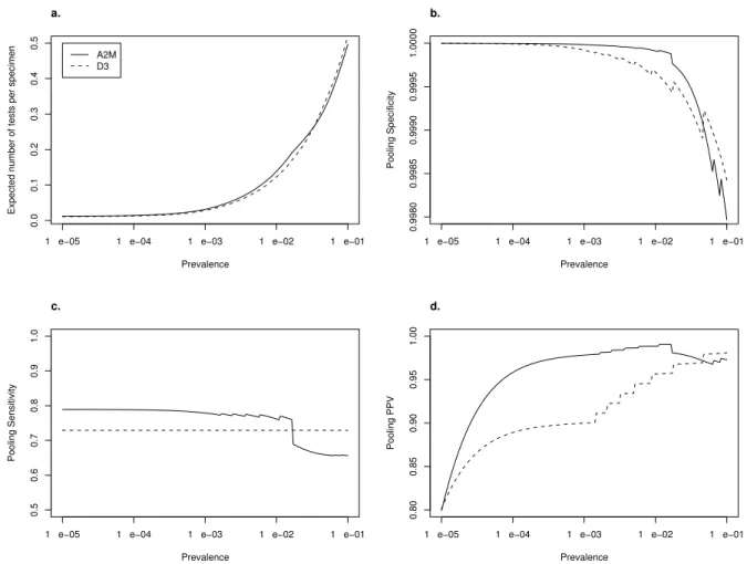
The results above suggest eitherD3 orA2M are generally preferable for detection of

acute HIV. Thus, we also consider how D3 andA2M compare for prevalences ranging

from 10−5 _{to 10}−1_{. As in the examples above, we assume}_Se _{= 0.9,} _Sp _{= 0.99, and the}

maximum allowable pool size is 100 due to dilution effects. Under these assumptions,

for each prevalence we found the values of n _{∈ {}4,9,16,25, . . . ,100_} that minimize

E_{D3(n : √n : 1)_} and E_{A2M(n : √n : 1)_}. The expected numbers of tests per

specimen, pooling specificities, sensitivities, andP P Vs at these optimal values ofn are

depicted in Figure 3.3. These results indicateA2M is generally the preferable algorithm

for prevalence less than 0.01.

The examples above assume that prevalence, test sensitivity, and test specificity

are known exactly, which will rarely be the case in practice. To account for such

uncertainty one can use a Bayesian analysis where priors are placed on p, Se and Sp

(e.g., see Dendukuri and Joseph (2001)). Alternatively one can employ a “sensitivity

analysis” wherein the operating characteristics of the pooling algorithms are examined

over a range of values forp,Seand/orSp. For example, suppose investigators in Malawi

are interested in the effect of the assumed values ofSe and Sp on the efficiency, pooling

sensitivity and poolingP P V ofD3(16 : 4 : 1). Then a graphical display such as Figure

3.4 can be used to showE(D3), Se(D3) andP P V(D3) over a bivariate range of values

ofSeandSp. Note Figure 3.4 includes the special case of no test error, i.e.,Se=Sp = 1.

(44)

presence of test error. Panels (b) and (c) demonstrate the more general phenomenon

that pooling sensitivity, specificity and predictive values equal 1 when Se=Sp = 1.

3.8 Discussion

We derived several operating characteristics of hierarchical and square array-based

test-ing algorithms for case identification in the presence of testtest-ing error. Ustest-ing these

results, we showed that the NC STAT program’s currently implemented pooling

algo-rithm D3(90 : 10 : 1) is approximately optimal among the algorithms considered here

with respect to the expected number of tests per specimen. However, moving to the

array-based pooling algorithmA2M(100 : 10 : 1) would generally improve pooling error

rates, in particular the expected number of false negatives (P F ER2), without

result-ing in a decrease in efficiency. Our results also suggest movresult-ing from D3(50 : 10 : 1) to

D3(16 : 4 : 1) in the Malawi setting would lead to substantial improvement in efficiency

as well as pooling error rates.

There are several areas of potential future research related to this work. First, we

assume constant sensitivity and specificity independent of pool size. This assumption

is not necessarily realistic and is highly dependent on individual disease and assay

characteristics. For HIV, the sensitivity of NAAT is likely inversely related to the

number of specimens per pool; as such, the applications above should be interpreted

with caution. Incorporating previously proposed methods of Hwang (1976) and Wein

and Zenios (1996) that allow sensitivity and specificity to be a function of pool size could

be considered for future research. Second, we have only considered two dimensional

square array algorithms. Generalizations to n _×m arrays with m ₆= n should be straightforward, however Berger et al. (2000) suggest m = n will be most efficient

in the absence of test error. Likewise, the proposed square array methods could be

(45)

extended to higher dimensional arrays in the presence of testing error. The efficiency

of higher dimensional arrays should simplify to the results given in Berger et al. (2000)

when Se =Sp = 1.

In summary, our results confirm that group testing algorithms can increase efficiency

and confer remarkable accuracy (predictive value) across a broad range of prevalence

in the presence of testing error. This ability of group testing algorithms to enhance

the accuracy of low prevalence disease screening is likely under-appreciated by clinical

laboratories. Of course, in clinical laboratory practice, functional constraints may affect

the pooling algorithm choice. For example, both the master pool size and the number

of test stages can affect the turn-around time for results. For investigators attempting

to evaluate the potential use of group testing algorithms for a particular application,

results such as ours can help estimate the trade-offs to be expected in terms of efficiency,

(46)

TABLE 3.1: Comparison of operating characteristics for individual testing and four potential pooling algorithms to be used in Malawi for detection of acute HIV.

A E₍A₎ S_p₍A₎ P CER₍A₎ S_e₍A₎ P CER₂₍A₎ P P V₍A₎ N P V₍A₎ IT∗ 1.00 0.9900 0.0096 0.9000 0.0045 0.8092 0.9953

D₃₍₅₀₎] _0.40 _0.9972 _0.0028 _0.7290 _0.0122 _0.9247 _0.9874 D₃₍₁₆₎† _0.32 _0.9989 _0.0010 _0.7290 _0.0122 _0.9696 _0.9874 A₂M₍₄₉₎‡ _0.34 _0.9995 _0.0005 _0.6810 _0.0144 _0.9836 _0.9852 A₂M₍₁₀₀₎§ _0.31 _0.9991 _0.0009 _0.6596 _0.0153 _0.9721 _0.9842

∗_{IT: Individual Test}

]_D_{3(50) :}_D_{3(50 : 10 : 1)}

†_D_{3(16) :}_D_{3(16 : 4 : 1)} ‡_A₂_M_{(49) :}_A₂_M_{(49 : 7 : 1)} §_A₂_M_{(100) :}_A₂_M_{(100 : 10 : 1)}

(47)

FIGURE 3.1: (a) Expected number of tests per specimen, (b) pooling specificity, (c) pooling sensitivity, (d) pooling P P V, (e) poolingP F ER, and (f) poolingP F ER2 for different algorithms assuming test sensitivity Se = 0.9, test specificity Sp = 0.99, and

prevalence p = 0.0002. The N _{denotes the three stage hierarchical pooling algorithm} employed in the NC STAT Program. Note pooling specificity for individual testing equals Sp = 0.99 and is not shown in panel (b).

0.005

0.020

0.100

0.500

n

Expected number of tests per specimen

4 9 16 25 36 49 64 81 100

Individual test A2 ( n:1) D2 (n:1) A2M (n: n:1) D3 (n: n:1)

a. 0.99970 0.99980 0.99990 1.00000 n Pooling Specificity

4 9 16 25 36 49 64 81 100

b. 0.70 0.75 0.80 0.85 0.90 0.95 1.00 n Pooling Sensitivity

4 9 16 25 36 49 64 81 100

c. 0.0 0.2 0.4 0.6 0.8 1.0 n Pooling PPV

4 9 16 25 36 49 64 81 100

d. 0.000 0.005 0.010 0.015 0.020 0.025 n Pooling PFER

4 9 16 25 36 49 64 81 100

e. 0.000 0.002 0.004 0.006 n Pooling P FE R2

4 9 16 25 36 49 64 81 100

(48)

FIGURE 3.2: (a) Expected number of tests per specimen, (b) pooling specificity, (c) pooling sensitivity, (d) pooling P P V, (e) poolingP F ER, and (f) poolingP F ER2 for

different algorithms assuming test sensitivity Se = 0.9, test specificity Sp = 0.99, and

prevalence p = 0.045. The N _{denotes the three stage hierarchical pooling algorithm}

employed in Malawi.

0.3 0.4 0.5 0.6 0.7 0.8 1.0 n

4 9 16 25 36 49 64 81 100

a.

Individual test A2 ( n:1) D2 (n:1) A2M (n: n:1) D3 (n: n:1)

0.990 0.992 0.994 0.996 0.998 1.000 n Pooling Specificity

4 9 16 25 36 49 64 81 100

b. 0.6 0.7 0.8 0.9 1.0 n Pooling Sensitivity

4 9 16 25 36 49 64 81 100

c. 0.80 0.85 0.90 0.95 1.00 n Pooling PPV

4 9 16 25 36 49 64 81 100

d. 0.0 0.2 0.4 0.6 0.8 n Pooling PFER

4 9 16 25 36 49 64 81 100

e. 0.0 0.5 1.0 1.5 n Pooling P FE R2

4 9 16 25 36 49 64 81 100

f.

(49)

FIGURE 3.3: (a) Expected number of tests per specimen, (b) pooling specificity, (c) pooling sensitivity, and (d) pooling P P V for optimally efficient configurations of D3 andA2M assuming test sensitivitySe = 0.9, test specificitySp = 0.99, and a maximum allowable pool size of 100.

1 e−05 1 e−04 1 e−03 1 e−02 1 e−01

0.0 0.1 0.2 0.3 0.4 0.5 Prevalence

a.

A2M D3

1 e−05 1 e−04 1 e−03 1 e−02 1 e−01

0.5 0.6 0.7 0.8 0.9 1.0 Prevalence Pooling Sensitivity c.

1 e−05 1 e−04 1 e−03 1 e−02 1 e−01

0.9980 0.9985 0.9990 0.9995 1.0000 Prevalence Pooling Specificity b.

1 e−05 1 e−04 1 e−03 1 e−02 1 e−01

(50)

FIGURE 3.4: Contour plots of (a) expected number of tests per specimen, (b) pooling sensitivity, and (c) pooling P P V for D3(16 : 4 : 1) assuming p= 0.045 as a function of test sensitivity (Se) and test specificity (Sp). The • denotes the values of Se and Sp

assumed in Table 3.1.

0.80

0.85

0.90

0.95

1.00

Test specificity (Sp)

Test sensitivity

(

Se

)

Test sensitivity

(

Se

)

.98 .99 1

a. Efficiency

.98 .99 1

b. Pooling Sensitivity

.98 .99 1

c. Pooling PPV

(51)

CHAPTER 4 THREE-DIMENSIONAL ARRAY

ALGORITHMS

4.1 Introduction

The focus of this chapter is to research aspects of three-dimensional array-based group

testing algorithms for case identification in the presence of test error.

Array-based algorithms were proposed by several researchers. Phatarfod and

Sud-bury (1994) derived the expected number of tests for two-dimensional array (i.e.,

ma-trix) group testing procedures. Berger et al. (2000) extended this work to higher

dimensional arrays assuming no test errors, i.e., no false negative or false positive tests.

In this chapter, we extend Berger et al. (2000)’s results to allow for imperfect

testing. We derive efficiency and pooling measurement error rates such as specificity

and sensitivity for three dimensional array-based pooling algorithms when there exist

test errors. Algorithms with and without master pool testing are considered. Our

Operating characteristics of group testing algorithms for case identification in the presence of test error