Boone_unc_0153M_15288.pdf

(1)

CALCULATION OF SENSITIVITY COEFFICIENTS USING CMAQ-DDM FOR INDIVIDUAL AIRPORT EMISSIONS IN THE UNITED STATES

Scott T. Boone

A thesis submitted to the faculty at the University of North Carolina at Chapel Hill in partial fulfillment of the requirements for the degree of Master of Science in the Department of Environmental Sciences and Engineering in the Gillings School of Global Public Health.

Chapel Hill 2015

Approved By: Marc Serre

(2)

(3)

ABSTRACT

Scott T. Boone: Calculation of Sensitivity Coefficients Using CMAQ-DDM for Individual Airport Emissions in the United States.

(Under the direction of Saravanan Arunachalam and Marc Serre)

The Community Multiscale Air Quality (CMAQ) model instrumented with the Direct Decoupled Method in three dimensions (DDM-3D), an advanced method for sensitivity analysis of chemical transport models, is used to quantify individual impacts of large and mid-size US airports on ambient air quality. Sensitivity coefficients are generated for six precursor species groups, allowing estimations of O₃and PM2.5concentrations from each of 66 individual airports. Airports were divided into groups, minimizing interference and allowing more airports to be analyzed while keeping total simulation runtimes as low as possible. Chorded aviation activity data from the Aviation Environmental Design Tool (AEDT) were used to generate speciated emissions along flight tracks during landing and takeoff (LTO) activities.

Sensitivity grids were generated for ozone and primary and secondary components of fine particulate matter for the 66 airports in the domain. Emissions from these airports account for 61% of flights and 77% of fuel burn in the 2005 AEDT inventory; sensitivities from these airports account for 73% of total aviation LTO PM2.5sensitivities and 57% of total aviation LTO O3 sensitivities in the domain. Aircraft LTO operations for all airports in the domain were found to be responsible for an increase in annual average PM2.5concentrations of

2.4×10−3µg/m3nationwide (0.038% of PM2.5concentrations from all sources), with this level climbing to as high as 0.025 µg/m3near major airports. Ozone concentrations displayed an annual domain average 8-hr max sensitivity of 1.8×10−2ppbv (0.036% of O₃concentrations from all sources).

Sensitivity to PM2.5precursor emissions from individual airports was often far-reaching.

(4)

Thirteen airports produced total PM2.5sensitivities in excess of 10−3µg/m3at 250km, and 52 airports produced sensitivities in excess of 10−4µg/m3at the same distance; sensitivities at these distances tend to be primarily composed of secondary species, while sensitivities closer to airports are balanced more evenly between primary and secondary species. Spatially-resolved estimation of PM2.5from NAS-wide aircraft LTO operations was calculated to be responsible for an excess all-cause mortality of 131 (95% CI: 121–142) deaths per year.

These individual airport sensitivities will be used in the future to generate further estimates of current health and economic impacts of aviation activity, and to inform policy decisions regarding growth and operations in the aviation sector.

(5)

ACKNOWLEDGMENTS

This work would not have been possible without additional effort, input and guidance from Saravanan Arunachalam, Sergey Napelenok, Matt Woody, Pradeepa Vennam, Shih Ying Chang, B.H. Baek, Carlie Coats, Mark Reed, Jared Bowden, Mohammad Omary, Seth Olsen, Jonathan Levy, Stefani Penn, Philip McDaniel, Amanda Henley, Marc Serre, William Vizuete and Daniel Rodriguez. This work used the Extreme Science and Engineering Discovery Environment (XSEDE), which is supported by National Science Foundation grant number ACI-1053575. The author acknowledges the Texas Advanced Computing Center (TACC) at The University of Texas at Austin for providing HPC resources that have contributed to the research results reported within this paper. This work was funded by the US Federal Aviation Administration (FAA) Office of Environment and Energy as a part of ASCENT Project 19 under FAA Award Number

13-C-AJFE-UNC-003 to UNC. The aviation emissions inventories used for this work were provided by US DOT Volpe Center and are based on data provided by the US FAA and EUROCONTROL in support of the objectives of the ICAO Committee on Aviation Environmental Projection CO₂Task Group. Any opinions, finding, and conclusions or recommendations expressed in this material are those of the author(s) and do not necessarily reflect the views of the US DOT, Volpe Center, the US FAA, EUROCONTROL, ICAO, ASCENT or its sponsors.

(6)

PREFACE

This work represents one end of a continuum of research conducted over the course of three years between the environmental sciences and transportation policy.

(7)

TABLE OF CONTENTS

LIST OF TABLES . . . viii

LIST OF FIGURES . . . ix

LIST OF ABBREVIATIONS . . . xi

1 BACKGROUND . . . 1

1.1 Aviation and air quality . . . 1

1.2 Sensitivity analysis and source apportionment . . . 2

2 METHODOLOGY . . . 9

2.1 Domain selection . . . 10

2.2 Data . . . 12

3 RESULTS & DISCUSSION . . . 14

3.1 Model evaluation . . . 14

3.2 Individual airport analyses . . . 22

3.3 Health impacts . . . 24

3.4 Limitations . . . 29

4 CONCLUSIONS . . . 31

APPENDIX . . . 33

REFERENCES . . . 153

(8)

LIST OF TABLES

Table 1 US air quality standards . . . 2

Table 2 Domain average contributions . . . 21

Table A1 List of 66 modeled airports and grouping . . . 36

Table A2 Monthly emissions totals . . . 37

Table A3 Sensitivity parameters for PM2.5precursor subspecies . . . 41

Table A4 CMAQ PM2.5output species . . . 41

Table A5 CMAQ model configuration . . . 42

Table A6 Aerosol species composition equations . . . 43

Table A7 CMAQ layer height levels . . . 44

Table A8 Comparison with monitoring networks. . . 66

(9)

LIST OF FIGURES

Figure 1 Forward and inverse sensitivity analysis . . . 8

Figure 2 Location of modeled airports . . . 11

Figure 3 Example vertical emissions profile . . . 12

Figure 4 Spatial comparison of secondary PM2.5species . . . 17

Figure 5 Spatial comparison of primary PM2.5species and O3 . . . 18

Figure 6 Seasonal NO₃response, CMAQ v4.7.1 vs CMAQ v5.0.1 . . . 19

Figure 7 Sensitivity of all PM2.5species to emissions from ATL . . . 23

Figure 8 Single-airport comparison . . . 24

Figure 9 Speciated annual average sensitivities . . . 25

Figure 10 Maximum sensitivity by distance (January) . . . 26

Figure 11 Maximum sensitivity by distance (July) . . . 27

Figure 12 Annual excess mortality . . . 29

Figure A1 Total January background emissions, NH₃ . . . 38

Figure A2 Total January background emissions, NO_x . . . 39

Figure A3 Total January background emissions, VOCs . . . 39

Figure A4 Total January background emissions, SO₂ . . . 40

Figure A5 Total January background emissions, primary PM2.5 . . . 40

Figure A6 Monthly total PM2.5and O3sensitivities . . . 45

Figure A7 Monthly PM2.5sensitivities . . . 46

Figure A8 Monthly O₃sensitivities . . . 47

Figure A9 Comparison between CMAQ-DDM 4.7.1 and CMAQ BF 4.7.1 . . . 48

Figure A10 Comparison between CMAQ-DDM 4.7.1 and CMAQ BF 5.0.1 . . . 49

Figure A11 Percent PM2.5from NOx . . . 50

Figure A12 Total sensitivity vs distance, all airports . . . 51

Figure A13 Monthly home PM2.5sensitivities (January) . . . 52

Figure A14 Monthly home PM2.5sensitivities (July) . . . 53

(10)

Figure A15 Monthly home O₃sensitivities . . . 54

Figure A16 Peak PM2.5sensitivities by airport . . . 55

Figure A17 Peak O₃sensitivities by airport . . . 56

Figure A18 PM2.5sensitivity by precursor (ATL) . . . 57

Figure A19 PM2.5sensitivity by precursor (ORD) . . . 58

Figure A20 PM2.5sensitivity by precursor (LAX) . . . 59

Figure A21 PM2.5sensitivity by precursor (JFK) . . . 60

Figure A22 O₃sensitivity by precursor (ATL) . . . 61

Figure A23 O₃sensitivity by precursor (ORD) . . . 62

Figure A24 O₃sensitivity by precursor (LAX) . . . 63

Figure A25 O₃sensitivity by precursor (JFK) . . . 64

Figure A26 Comparison with monitoring networks (PM2.5) . . . 67

Figure A27 Comparison with monitoring networks (O₃) . . . 68

Figure A28 Comparison of O₃values with monitor observations . . . 69

Figure A29 Comparison of NO₃values with monitor observations . . . 70

Figure A30 Comparison of SO₄values with monitor observations . . . 71

Figure A31 Comparison of NH₄values with monitor observations . . . 72

(11)

LIST OF ABBREVIATIONS

AEDT Aviation Environmental Design Tool

BF Brute Force method, a.k.a. the subtractive, finite difference or zero-out method CAMx Comprehensive Air quality Model with eXtensions

CB05 Carbon Bond 05 chemical mechanism (Yarwood et al., 2005) CMAQ Community Multiscale Air Quality model

CTM Chemical Transport Model DDM Decoupled Direct Method EBI Euler Backwards Integration HD-DDM High Dimension (or order) DDM

ICAO International Civil Aviation Organization ISAM Integrated Source Apportionment Method LTO Landing and Takeoff Operations

PM2.5 Particulate Matter of diameter less than 2.5 µg/m3 NAAQS National Ambient Air Quality Standards

NAS National Air Space

PSAT Particulate Source Apportionment Technology SMOKE Sparse Matrix Operator Kernel Emissions TSSA Tagged Species Source Apportionment method WRF Weather Research and Forecasting model

(12)

1 BACKGROUND

1.1 Aviation and air quality

Aviation is a critical segment of the U.S. transportation sector, growing in both absolute and relative terms. Between 2001 and 2011, the share of domestic passenger-miles traveled by air increased from 9.5% to 11.8% compared to terrestrial and marine modes (Bureau of

Transportation Statistics, 2014a). Over the same period, air carriers saw growth of about 17%, with nearly 578 billion domestic passenger miles traveled in 2013 (Bureau of Transportation Statistics, 2014b).

Aircraft, like all vehicles fueled by combustion of petrochemicals, emit polluting chemicals into the atmosphere. Fine particles are emitted directly from engines in the form of soot and dust, while oxidation of emitted nitrates, sulfates and organic compounds leads to the formation of O₃and secondary particulate matter. Ground-level O₃1and fine particulate matter2 are two of six federally-regulated air pollutants with known adverse impacts on human health (table 1). Major airports in the US are often located in or near major population centers. Human exposure to O₃and PM2.5can cause chronic and acute disease in the form of asthma, bronchitis, cardiopulmonary disease and cancer. Large-scale cohort studies have found that a

10 µg/m3increase in ground-level PM2.5concentrations is associated with an approximately 10% increase in all-cause mortality (Pope III et al., 2002; Jerrett et al., 2009).

1_{Throughout this work, chemical species set in standard type (e.g. NH}

4) refer to actual chemical species, whereas

species set inmonospace(e.g.ANH4IJ) refer to modeled pseudo- or super-species.

2_{Particulate matter (also referred to as aerosol, though this term properly refers to both the particulate and the gas}

in which it is suspended) is a catch-all term for any solid- or liquid-phase matter suspended in the atmosphere. Particulate matter of diameter less than 2.5 microns is known as PM2.5; this size roughly corresponds to the sum

of computer-simulated Aiken and Accumulation modes (PMIandPMJ, respectively;PMIJ, collectively) and the two terms are used more or less interchangeably in this document (Binkowski and Roselle, 2003).

(13)

Pollutant Averaging Time Level Form

Ozone3 8-hour 75 ppbV Annual fourth-highest daily maximum 8-hr concentration, averaged over 3 years PM2.5 Annual 12 µg/m3 Annual mean, averaged over 3 years

PM2.5 24-hour 35 µg/m3 98th percentile, averaged over 3 years

Table 1: US National Ambient Air Quality Standards (NAAQS) for O₃and PM2.5.

Previous estimation of aviation’s contribution to O₃and PM2.5showed that in 2005, about 0.05% of average ambient PM2.5levels could be linked to aircraft landing and takeoff operations (LTO), with this value rising to 0.11% by 2025 (Woody et al., 2011). Impacts near airports are significantly higher, with proportion of ambient PM2.5attributable to aircraft LTO approximately doubling compared to regions located more distantly from an airport; however, adverse air quality and health impacts can be seen as far as 200–300 km away from airports (Arunachalam et al., 2011). While aircraft operating at cruise altitude also have significant impacts on air quality and health—up to 80% of the total global impacts of aviation—these impacts are seen at the

intercontinental level due to the large transport distances involved (Barrett et al., 2010).

Model-based calculations of annual excess mortality from LTO have estimated that in 2005, 75 premature deaths were caused by aircraft LTO at 99 major US airports, a number expected to rise to 460 in 2025 (Levy et al., 2012).

Because airports differ wildly in both their level of activity and proximity to population centers, it is important to assess their contributions to ground-level PM2.5and O3concentrations on an individual level. Previous work has assessed either a few airports individually or the sector as a whole; this goal of this work is to provide concurrent individual estimations of the impacts of the majority of large and medium airports in the continental US.

1.2 Sensitivity analysis and source apportionment

Eulerian Chemical Transport Models (CTMs) function by modeling the atmosphere as a series of well-mixed three-dimensional grid cells. At each modeled timestep, the effects of 3_{Likely to be revised per current standing proposal by the EPA (US Environmental Protection Agency, 2014).}

(14)

meteorological, chemical, and physical processes are evaluated within and between grid cells, giving discrete values for the chemical concentrations of each modeled species. These values are then aggregated to provide hourly, daily, monthly or annual estimates of atmospheric conditions which can be used to estimate health, ecologic and economic impacts of atmospheric pollutants. This work uses the Community Multiscale Air Quality model (CMAQ) (Byun and Schere, 2006); other, similar CTMs include the Comprehensive Air Quality Model with Extensions

(CAMx) (ENVIRON, 1998) or the global-scale GEOS-Chem (Bey et al., 2001).

In an Eulerian CTM, chemical concentrations for each species are governed by the basic advection-reaction-dispersion equation (Jacobson, 2005). At each time step and for each grid cell and species, the model evaluates the following equation:

∂

∂tYi=−∇(uYi) +∇(K∇Yi) +Ri+Ei

whereYirepresents a chemical species,urepresents velocity of the medium,K the diffusivity

tensor,Rithe reaction rates, andEithe emissions rate.

Research using CTMs generally uses one of two methods to both calibrate models to observations and quantify impacts of various emissions or environmental scenarios: source apportionment and sensitivity analysis. Source apportionment seeks to track modeled species through time, space and chemical transformation, either by observing the changes to the system when those species are removed entirely, or by tagging emitted species and following them through the CTM system. Outputs from a source apportionment procedure are chemical concentrations that represent the difference∆Yibetween scenarios:

∆Y_i=Y_i_sens−Y_i_base

Sensitivity analysis can be considered a conceptual generalization of source apportionment techniques. Rather than tracking the fate and transport of specific chemical entities, sensitivity analysis determines the mathematical effects of perturbation of model input parameters on model

(15)

outputs. Changes in inputs are not limited to changes in emissions rates, but can also include model parameters such as chemical reaction rates, meteorological conditions or model initial and boundary conditions. Sensitivity analysis, in contrast to source apportionment, can help to capture nonlinear interactions between species in a CTM. Outputs from a sensitivity analysis procedure are sensitivity coefficients; like the deltas calculated by source apportionment, sensitivity coefficients are in concentration units, however they represent coefficientsC_i_,_jto be applied to equation of the form

Y_i_sens=Y_i_base+∆x_j·C_i,j

such thatY_i_baseis the unadulterated model output resulting from inclusion of all unperturbed model inputs and∆xjrepresents the scale factor or perturbation applied to input parameterXj. If

∆xj=0, then no perturbation is applied, andYisens=Yibase. A scale factor of -1 would represent the “zero-out case”, and a scale factor of 0.2 would represent a 20% increase in parameterXj.

Source apportionment and sensitivity analysis of CTMs form the heart of model-based air quality analysis. A number of implementations of these two methods exist, each balancing

computational complexity, flexibility, and precision of results. We can further distinguish between methods by their implementation. Methods that use standard CTM outputs with no additional modules loaded can be considered “outside the model” methods. Methods requiring changes or additions to the CTM codebase can be considered “inside the model”. Finally, methodologies can be divided into source- or receptor-based methods. Source-based methods identify the results of changes in input on output, while receptor-based (or inverse) methods calculate the required changes in input to produce a change in output.

Brute force The brute force method (also known as the subtractive or zero-out method) is the simplest form of source apportionment and the method by which all others are evaluated. In the brute force method, a “base case” model run is conducted with all emissions included; subsequent model runs (“sensitivity cases”) either add or remove scenario-based emissions of interest (e.g., the emissions from a single sector). The subtractive difference between the base and sensitivity

(16)

cases is then used to identify changes in output concentrations caused by the addition or subtraction of emissions in each sensitivity case.

The brute force method has two major advantages: it is conceptually simple and, for a single scenario, extremely accurate. Indeed, the brute force method is generally the method to which other sensitivity analysis methods are compared and calibrated. However, it has several drawbacks. It is not possible to extrapolate results from model outputs; each scenario requires a separate model run beyond the base case, meaning that fornscenarios,n+1 modeling runs must be conducted. This means that computation time increases linearly with the number of scenarios desired.

Regression-based Regression-based methods, such as the Response Surface Method (RSM) use a series of model runs with carefully-chosen variation in key parameters to build a least-squares regression model linking changes in model input to changes in model output (Box and Draper, 1987). The RSM is the logical next step in overcoming the limitations of the brute force method, allowing interpolation between individual model runs created by varying model inputs (Masek, 2008; Xing et al., 2011; Ashok et al., 2013; Brunelle-Yeung et al., 2014; Wang et al., 2011).

Whereas brute force methods do not allow for multiple scenarios to be evaluated from a single suite of model runs, RSM-derived regression coefficients can be used with a variety of emissions scenarios. However, alternative scenarios must be contained within the sample space used to create the training runs. In order to construct a response surface, a range of input values (typically at least three) fornparameters must be chosen in order to create ann−dimensional sample space spanning the desired set of scenarios. Depending on the sampling methodology used, expansion of the sample space may cause the existing set of training runs to become unbalanced, requiring an entirely new set of training runs to be conducted (Masek, 2008).

In order to provide policy-oriented context to output from sensitivity analysis, Bayesian statistical methods can be used to account for bias and error in the CTM results and then combine results from modeling exercises with data from monitoring networks. These methods take

(17)

advantage of the accuracy and verifiability of monitoring networks while retaining the domain extent and scenario-evaluating abilities of modeling exercises (Foley et al., 2012).

Tracer and tagged-species methods Tracer methods follow inert species such as primary particulate matter through the transport modules of the CTM. Tagged-species methods, such as the Tagged Species Source Apportionment method (TSSA) (Wang et al., 2009) for CMAQ or the Particulate Source Apportionment Technology (PSAT) (Yarwood et al., 2007) for CAMx track chemical species (sometimes called reactive tracers) through the gas and aerosol chemistry modules of the CTM, allowing the additional analysis of reactive species such as O₃and

secondary PM2.5. Inverse applications of tracer methods are known as back trajectory modeling; implementations such as HYSPLIT follow species trajectories backwards in time (Draxler and Rolph, 2003).

The Integrated Source Apportionment Method, or ISAM, is an updated implementation of TSSA with streamlined input requirements and improvements in dry/wet deposition

tracking (Kwok et al., 2013, 2015). Tagged species methods can account for some of the nonlinearity in chemical processes lost using the brute force method. However, this method is weaker for difficult-to-model nonlinear reactions such as nitrate formation. ISAM can be used for analysis of emissions (either location- or sector-specific) and boundary conditions.

Decoupled Direct Method The Decoupled Direct Method in three dimensions (DDM-3D) is an inside-the-model sensitivity analysis method that has been implemented in several

CTMs (Dunker, 1984; Hakami et al., 2003; Cohan et al., 2005; Napelenok et al., 2006). In DDM, one or more model parameters are tagged as sensitivity parameters (e.g. emissions, boundary conditions or reaction rates). During the model run, a sensitivity coefficient will be generated for each output species linking its concentration to perturbations in the respective input parameter. Numerically, the equation

C_i,j=

∂Yi

∆∂xj

(18)

represents the sensitivityC_i,j of the concentration of speciesYito a perturbation∆xj as applied to

sensitivity parameterXj. Sensitivities are calculated in the same method as the

advection-reaction-dispersion equation:

∂

∂tCi,j=−∇(uCi,j) +∇(K∇Ci,j) +JiCi,j+Ei

whereJ is the corresponding row from the Jacobian matrix representing interspecies chemical interaction kinetics. It is important to note that the Jacobian must be calculated (unless its rate of change is quite slow) for each timestep (Dunker, 1984). DDM is source-oriented in that it calculates sensitivities ofallmodel output species across the domain to each targeted sensitivity parameter; in other words, it comprehensively determines the effects of a few designated model inputs.

Higher-order implementations of DDM in CMAQ (HD-DDM) have been released, allowing nonlinear processes and cross-sensitivities to be better captured by the model and generating sensitivity coefficients of the form:

C_i_,_j_,_k= ∂

2_Y

i

∂∆xj∆∂xk

,

where the product of perturbations in sensitivity parametersXj andXkis linked to output species

Yi(Cohan et al., 2005; Zhang et al., 2012). First-order DDM has been shown to compare

favorably in output with brute force calculations for reductions of up to 20% for both primary and secondary emissions (Koo, 2011). For very small (<10%) perturbations, DDM may in some cases be superior to the brute force method due to numerical noise present between the two slightly different runs required for that method (Napelenok et al., 2006).

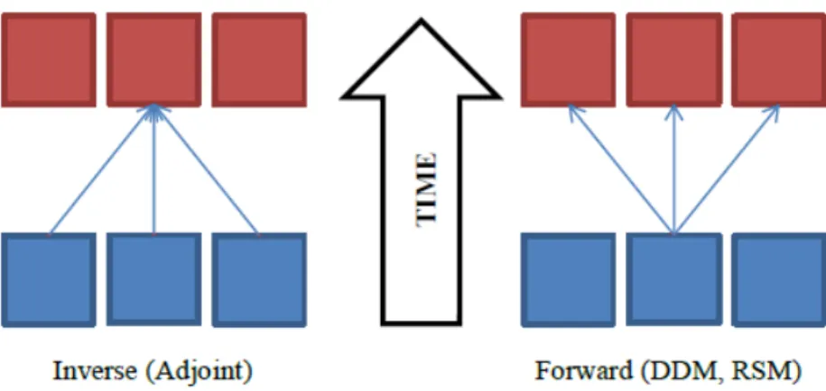
The closely-related adjoint method uses the sensitivity coefficients generated by DDM to perform receptor-based (also known as inverse) sensitivity analysis (Hakami et al., 2007). Instead of calculating the results of a few perturbations in inputs on the entire model output, the adjoint method calculates the required perturbations of inputs to cause a given model output (figure 1).

(19)

Figure 1: Inverse methods predict the perturbations on all input points (blue) required to generate an impact on a single output point (red), while forward methods measure effects of perturbation of a single input across the output domain (adapted from Koo (2011)).

The adjoint method is well-suited to determining the effects of a wide range of model inputs on a specific region—for example, calculating the impacts of worldwide aviation emissions (both during LTO activity and while at cruise altitude) on regional surface air quality and health (Koo et al., 2013). Other applications of the adjoint method include refining emissions inventories based on observations from monitoring networks by finding the error between receptors (both model outputs and observations) and their upstream sources (emissions inventories) (Henze et al., 2009).

(20)

2 METHODOLOGY

The goal of this work is to use the CMAQ model instrumented with the decoupled direct method to characterize individual airport contributions due to aircraft LTO operations to ambient air quality from large and mid-size airports in the United States, and to produce a dataset that can be used to calculate the air quality and health impacts of various aviation activity scenarios. An approach based on the DDM-instrumented version of CMAQ was selected for several reasons. First, DDM has shown strength in calculating sensitivities for a relatively large number of

parameters in a single model run, reducing the quantity of runs that must be conducted compared to brute force and regression-based methods. Second, the relatively small quantity of emissions emitted by each source (i.e., airport) make DDM an appropriate choice, minimizing the model noise created by the multiple base and sensitivity cases required by the brute force method. Use of DDM allows for future extensibility relative to regression-based methods, allowing more airports to be added to the study at a future date without requiring any already-completed modeling to be re-run in order to address sampling balance issues. While regression-based methods can have superior performance for very larger perturbations (60–90%) (Foley et al., 2014), this work focuses on a subset of the aviation sector, which composes a very small (<1%) proportion of total air pollutant emissions in the US (table A2).

Finally, use of a forward sensitivity analysis method (such as DDM) as opposed to an inverse method (such as the adjoint method) is appropriate due to the source-oriented (i.e., impacts across the domain of a specific set of airports) nature of this work. A similar

methodology using the adjoint method might focus on a subregion of the US and determine the degree to which all US airports affect air quality in that region. Both forward and inverse methods selectively solve the set of influences of all sources on all receptors (i.e., the Jacobian with respect

(21)

to all emissions species, output species, grid cells, and time steps). Forward methods constrain the set of inputs—in our case, a subset of emissions from airports—and calculate sensitivity

coefficients for all model outputs with respect to this list. Inverse methods take the opposite approach by constraining the set of observed model outputs, but calculating the effects of all inputs on that set. Other efforts to quantify the contribution of aviation to date have focused on the impact of emission from the entire aviation sector on a more limited set of receptors, and so are better suited to use of inverse methods. For example, the adjoint method has been used to calculate the effects of worldwide cruise emissions on regional air quality, allowing

region-specific source apportionment and health impact analysis (Koo et al., 2013).

A modeling framework was created to quantify the contributions of individual airports during the year 2005 and generate sensitivity coefficients for O₃and PM2.5to evaluate the impacts of variations in these emissions.

2.1 Domain selection

Airports were selected for modeling in order to capture as much of US aviation activity as possible, both in terms of spatial coverage and absolute emissions. Because each additional sensitivity parameter represents a linear increase in processing time, airports distant enough to not create overlapping sensitivity plumes were combined into sensitivity groups where possible. Preliminary CMAQ-DDM runs were conducted for 139 individual candidate airports in order to find compatible airport groups. Each simulation was run for six days (including a one-day spinup period) in the first week of January and the first week of July. The two five-day result sets were averaged to create approximate annual sensitivity grids to be used for selecting airports whose PM2.5plume interactions were minimal. Allocation of airports was done with a mix of

algorithmic randomized pairing and manual fine-tuning and selection of groups. Groups were selected in order to avoid an overlap of any area of PM2.5sensitivity greater than 10−5µg/m3, a concentration well below detection limits of particulate matter monitoring equipment (Chow et al., 2008).

(22)

In total, 66 airports were chosen and allocated among 30 sensitivity groups, each group containing between one and four airports (table A1). These airports represent 77% of annual fuel burn4within the US National Air Space (NAS) as reported by the FAA’s Aviation Environmental Design Tool (AEDT) (Roof et al., 2007; Wilkerson et al., 2010). An additional group was created containing emissions from all airports in the continental United States, for a total of 31 groups. Because aviation LTO emissions represent far less than 20% of all PM2.5precursor emissions, our calculated sensitivity coefficients should be sufficiently accurate for perturbations of at least ±100% of aviation emissions.

! ! ! ! ! ! ! ! ! ! ! ! ! ! ! ! ! ! ! ! ! ! ! ! ! ! ! ! ! ! ! ! ! ! ! !! ! ! ! ! ! ! ! ! ! ! ! ! ! ! ! ! ! ! ! ! ! ! ! ! ! ! ! ! !

Figure 2: Location of 66 individually-modeled airports.

For each airport group, six precursor species groups (NO_x, SO₂, VOCs, PSO₄, PEC and POC; table A3) were designated as sensitivity input parameters5, for a total of 186 sensitivity parameters. Flight segment data from AEDT were processed into gridded emission rate files using AEDTProc (Baek et al., 2012). Full-flight aircraft emissions were capped at 3,000 feet (about 914 meters) in order to only capture landing and takeoff operations. A separate emissions file was created for each airport group to be tagged as a set of sensitivity parameters for a given DDM run. Creating separate files, as opposed to tagging emissions from a single vertical column 4_{During LTO operations.}

5_{Sensitivity of O}

3was calculated for NOxand VOC emissions only.

(23)

containing the airport, allowed the capture of the roughly conic flight emissions profiles generated by aircraft taking off and landing at each airport (figure 3).

The physical domain used a modeling grid of 36×36 km horizontal resolution covering the continental United States (CONUS). Thirty-four vertical layers (time-varying based on atmospheric pressure, with the top layer keyed to an atmospheric pressure of 50 mb) were used (table A7).

Figure 3: An example of vertical variation in aviation emissions around an airport—in this case, annual average NO_x (left) and primary elemental carbon (right) emissions rates (in tons per day) from Denver International Airport (DEN). The bulk of emissions are at ground level, but note the horizontal emissions profile that extends east (i.e., along increasing column numbers) reflecting flight paths. Shown are vertical CMAQ layers 1 through 17 along domain row 59. CMAQ includes 34 vertical layers, but LTO emissions are limited to the first 17 (table A7).

2.2 Data

Background emission rates for other anthropogenic sources from EPA’s National Emissions Inventories (NEI-2005) were processed into grid-based emissions using the Sparse

(24)

Matrix Operator Kernel Emissions Model (SMOKE) (U.S. Environmental Protection Agency, 2005). Boundary conditions were derived from global CAM-chem simulations for the year 2005 (Lamarque et al., 2011), which also used the same AEDT-based globally chorded aircraft emissions inventories. Meteorology for 2005 was obtained from the Weather Research and Forecasting model (WRF) (Skamarock et al., 2005), with outputs downscaled from NASA’s Modern-Era Retrospective Analysis for Research and Applications data (MERRA) (Rienecker et al., 2011). CMAQ v4.7.1 with first-order DDM-3D was used to generate sensitivity and concentration output files. Two other versions of CMAQ were used for model verification purposes: CMAQ v5.0.1, a version containing the most (at the time) up-to-date chemistry and other science modules, and a non-DDM version CMAQ 4.7.1 with an otherwise identical configuration (table A5) (Byun and Schere, 2006; Napelenok et al., 2006). Modeling was conducted on NSF XSEDE’s Stampede compute cluster (J. Towns, 2014). Additional archived model runs (those using CMAQ v5.0.1) were conducted on UNC’s Killdevil compute cluster.

The model was run for one month each in January and July of 2005, with an eleven-day spin-up period used to generate initial conditions. These two months were chosen to represent winter and summer seasons, and the average of these two month-long simulations is used to provide an estimate of annual average sensitivities for 20056.

6_{For the remainder of the this work, “annual average” refers to the average of January and July—a pseudo-average—}

rather than a true twelve-month averaging period.

(25)

3 RESULTS & DISCUSSION

3.1 Model evaluation

We evaluated our model in three ways: first, base (i.e., non-DDM) model output was compared to observational data. Next, DDM and brute force model outputs from the spin-up period were compared against each other to establish the relationship between the two methods when run with identical input data. Finally, we compared full January and July DDM runs against previously-completed brute force modeling runs conducted over the same temporal domain.

3.1.1 Evaluation against observations

We first evaluated model output from the base CMAQ model with no sensitivity analysis or source apportionment instrumentation included in order to evaluate its effectiveness at

capturing general atmospheric conditions. Gridded model outputs were compared with

spatiotemporally-resolved point observations from several monitoring networks, including the Air Quality System (AQS) network for O₃and for PM2.5measurements, the Clean Air Status and Trends Network (CASTNet), Interagency Monitoring of Protected Visual Environments

(IMPROVE) network and the SouthEastern Aerosol Research and Characterization (SEARCH) Network.

Model outputs for most species had normalized median error7of 50% or less, indicating fair agreement with monitoring sites (for full results and comparisons against other, similar exercises, see table A8). The exception was NO₃, which had generally poor model performance and showed higher normalized median error values. However, the accurate modeling of nitrate 7_{NMdE, calculated as} ∑Median(Mod−Obs)

∑Median(Obs) .

(26)

aerosol production when compared to monitor data—especially in the winter—has been consistently challenging, with errors in the prediction of other aerosol species affecting nitrate performance (Yu et al., 2005). Regional overestimation of nitrate in the western US may be related to the complex topography and meteorological conditions found there (Baker et al., 2011). However, updates to the aerosol mechanism in CMAQ have continued to improve model

performance for secondary PM2.5species over time (Simon et al., 2012).

3.1.2 Evaluation against spin-up brute force runs

As described above, outputs from sensitivity analysis experiments are often first compared to results from similar analyses conducted using brute force methods. We first evaluated our DDM output by comparing the NAS-wide all-airport sensitivity coefficients with results from brute force runs conducted along the same temporal domain as model spin-up period using an otherwise identical setup (figures A9).

DDM sensitivities8of gas-phase and primary aerosol species to airport emissions compare well with brute force runs, with cell-by-cell R2above 0.9 for each pairwise comparison of O₃and

AEC(figure A9). Sensitivity of secondary PM2.5species to emissions showed significantly less agreement between each analysis method. All secondary species performed poorly in the winter (R2<=0.5), but summer values were generally better (R2around 0.9). Note the relative lack of negative ammonium and nitrate values in DDM output when compared to brute force runs, a characteristic that has been explained as the result of numerical diffusion between adjacent fields in the latter method (Hakami et al., 2004; Cohan et al., 2005; Napelenok, 2006).

8_{There is an important distinction to make in the interpretation of results from DDM. As stated above, DDM calculates}

sensitivity coefficients linking outputs to inputs, which means that each value reported by the model is linked to two species: an input species and an output species (the input parameter need not be an actual chemical species—it could be another model parameter—but in this work, input parameters will always constitute a species or group of species). Further, in this work, inputs or outputs will generally be aggregated together: either as sensitivity of all output PM2.5species to a specific precursor, or sensitivity of a specific model output species to all precursors. In

some cases—particularly nonreactive primary PM2.5species— (1) the sensitivity of all outputs to a single input and

(2) the sensitivity of a single output to all inputs will be nearly identical; in the case of more mutually-reactive species displaying nonlinear behavior, the two will be different. When comparing DDM results to those of brute force model runs, sensitivities of output species to all emissions will be compared to the same output species from the brute force runs. When interpreting DDM results on their own, sensitivities of total PM2.5will be reported in terms of each input

parameter separately.

(27)

3.1.3 Evaluation against other brute force runs

Agreement is similar when compared to archived full month-long (January and July) work previously completed on a different platform (CMAQ 5.0.1, with changes to aerosol chemistry and addition of lightning-generated NO_xemissions) (figure A10). As with the CMAQ v4.7.1 comparisons, O₃and primary PM2.5are in good agreement, with secondary species performing more poorly. When disaggregated by species, these differences are largely due to over-predictions in sensitivities to NO_xemissions, especially far downwind from emission sites. Modeling

sensitivity of secondary inorganic PM2.5species (e.g. nitrate and ammonium species) using DDM often compares poorly to BF output, but could potentially be improved with the use of

higher-order DDM (Koo et al., 2009).

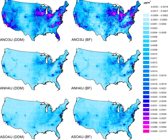
Total PM2.5by precursor appears to be dominated by sensitivity to NOxon a national scale, but sensitivities to individual precursors are much more balanced near airports (figure A11). In general, aircraft from DDM model runs showed over-prediction of nitrate-based aerosol and slight over-prediction of ammonium aerosol (especially in the southwestern US) and an

under-prediction of sulfate aerosol when compared with brute force model runs (figure 4). Because of differences in the two base models—runs conducted with CMAQ v4.7.1 used the Aero5 aerosol module, while those conducted with CMAQ v5.0.1 used the Aero6 module—some of the differences between these two sets of runs may be more attributable to differences in the base model rather than the sensitivity analysis technique used. CMAQ v4.7.1 produced more winter nitrate aerosol overall in the southwestern US when base model runs between the two modeling setups are compared (figure 6).

Secondary PM2.5plumes—particularly nitrate aerosol—over Iowa, central California, southeastern North Carolina, and Upstate New York can be explained by excess free ammonia emissions in those regions (figure A7) (Woody et al., 2011). In general, the magnitude of both PM2.5and O3sensitivities was greater in July, likely due to increases in both aviation activity and photochemical ozone and secondary PM2.5production.

It is important to keep in mind that the subtractive source-specific concentrations obtained

(28)

μg/m3

-0.0033 - -0.0018 -0.0017 - -0.0007 -0.0006 - -0.0002 -0.0001 - 0.0000 0.0001 - 0.0002 0.0003 0.0004 - 0.0005 0.0006 0.0007 0.0008 0.0009 0.0010 0.0011 0.0012 0.0013 0.0014 0.0015 - 0.0016 0.0017 0.0018 - 0.0019 0.0020 - 0.0021 0.0022 - 0.0024 0.0025 - 0.0026 0.0027 - 0.0030 0.0031 - 0.0035 0.0036 - 0.0041 0.0042 - 0.0048 0.0049 - 0.0057 0.0058 - 0.0067 0.0068 - 0.0094 0.0095 - 0.0173

ANO3IJ (DDM) ANO3IJ (BF)

ANH4IJ (DDM) ANH4IJ (BF)

ASO4IJ (DDM) ASO4IJ (BF)

Figure 4: Spatial comparison of secondary PM2.5species from annual average DDM model runs (reported in

sensi-tivities, left) and brute force model runs (reported as differences in concentration between base and sensitivity cases, right). See table A4 for species compositions.

(29)

μg/m3

-0.0001 - 0.0000 0.0001 - 0.0000 0.0001 - 0.0000 0.0001 0.0002 - 0.0001 0.0002 - 0.0001 0.0002 - 0.0001 0.0002 0.0003 - 0.0002 0.0003 - 0.0002 0.0003 0.0004 - 0.0003 0.0004 0.0005 0.0006 0.0007 - 0.0009 0.0010 - 0.0013 0.0014 - 0.0045

AOMIJ (DDM) AOMIJ (BF)

AECIJ (DDM) AECIJ (BF)

O3 (DDM) O3 (BF)

ppbV

-0.66 - -0.54 -0.53 - -0.16 -0.15 - -0.07 -0.06 - -0.01 0.00 0.01 0.02 0.03 0.04 - 0.06

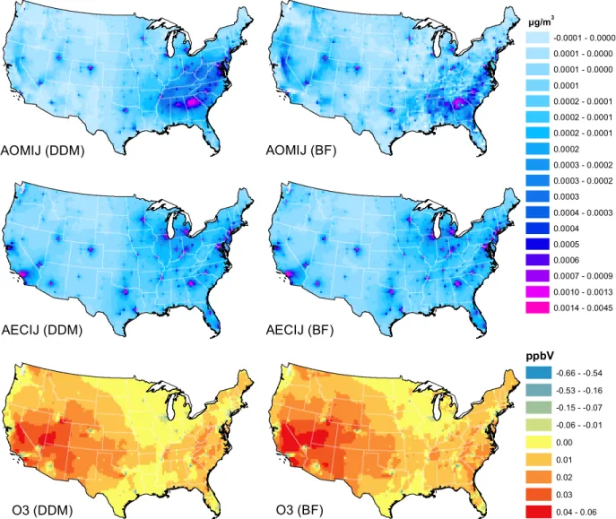
Figure 5: Spatial comparison of primary elemental carbon, organic PM2.5and O3from pseudo-annual average (i.e.,

January and July averaged together) DDM model runs (reported in sensitivities, left) and brute force model runs (reported as differences in concentration between base and sensitivity cases, right). See table A4 for species composi-tions.

(30)

ANO3IJ ug/m3

0.31 - 0.86 0.87 - 1.23 1.24 - 1.67 1.68 - 2.15 2.16 - 2.68 2.69 - 3.31 3.32 - 4.07 4.08 - 5.02 5.03 - 6.22 6.23 - 8.36

CMAQ v4.7.1 (JAN) CMAQ v5.0.1 (JAN)

CMAQ v4.7.1 (JUL) CMAQ v5.0.1 (JUL)

Figure 6: Comparison between seasonal overall (i.e., including emissions from all sources) NO₃aerosol production from CMAQ v4.7.1 (left) and CMAQ v5.0.1 (right) in January (top) and July (bottom). Note the higher January NO₃ concentrations in the southwestern US produced by CMAQ v4.7.1.

(31)

from brute force methodologies do not necessarily reflect their real-life contributions to air quality more accurately than do sensitivities obtained from DDM. In some cases, results obtained from DDM runs are more reasonable than similar brute force runs (Napelenok et al., 2006). When DDM outputs calculating the sensitivity across the domain to single airports were compared to similar outputs conducted using a brute force methodology, the DDM outputs displayed substantially less numeric noise at long distances from the airport (figure 8).

(32)

January July

30 All 30 Grp./ All All Apt./ 30 All 30 Grp./ All All Apt./

Groups Airports All Apt. Sources All Src. Groups Airports All Apt. Sources All Src.

O₃(8-hr max ppbV) -0.0030 -0.0041 74% 42.16 -0.010% 0.0299 0.0401 75% 57.26 0.070%

O₃(NO_x) -0.0035 -0.0052 68% 0.0292 0.0389 75%

O₃(VOC) 0.0013 0.0022 57% 0.0011 0.0017 68%

PM2.5(µg/m3) 0.0019 0.0028 69% 6.96 0.040% 0.0017 0.0021 79% 5.81 0.036%

PM2.5(Pri.) 0.0001 0.0001 75% 2.89 0.005% 0.0001 0.0001 119% 2.69 0.005%

PM2.5(Sec.) 0.0018 0.0026 69% 4.06 0.065% 0.0015 0.0020 77% 3.12 0.063%

PM2.5(NOx) 0.0017 0.0025 68% 0.0011 0.0015 71%

PM2.5PEC 0.0001 0.0001 74% 0.0001 0.0001 112%

PM2.5(POC) 0.0000 0.0001 75% 0.0001 0.0001 129%

PM2.5(PSO4) 0.0000 0.0000 87% 0.0001 0.0001 111%

PM2.5(SO2) 0.0000 0.0000 95% 0.0003 0.0003 83%

PM2.5(VOC) 0.0001 0.0001 81% 0.0000 0.0000 732%

Annual Average

30 All 30 Grp./ All All Apt./

Groups Airports All Apt. Sources All Src.

O₃(8-hr max ppbV) 0.0135 0.0180 75% 49.71 0.036%

O₃(NO_x) 0.0128 0.0169 76%

O₃(VOC) 0.0012 0.0019 61%

PM2.5(µg/m3) 0.0018 0.0024 73% 6.38 0.038%

PM2.5(Primary) 0.0001 0.0001 95% 2.79 0.005%

PM₂.5(secondary) 0.0017 0.0023 72% 3.59 0.064%

PM2.5(NOx) 0.0014 0.0020 69%

PM2.5PEC 0.0001 0.0001 91%

PM2.5(POC) 0.0001 0.0001 99%

PM2.5(PSO4) 0.0001 0.0001 104%

PM2.5(SO2) 0.0002 0.0002 84%

PM2.5(VOC) 0.0000 0.0000 131%

Table 2: Domain average contributions over the continental United States from 30 aggregated group runs, all airports in a single run, and the percentage of all airport activity represented by the 30 groups; followed by total all-sector concentrations, and the percentage of all-sector concentrations caused by aviation LTO.

(33)

Sector-wide and NAS-wide results compare reasonably well with previous estimations of aviation’s contribution to air quality in the US. Woody et al. estimate a total contribution from 99 major US airports of 3.2×10−3µg/m3, or about 0.05% of total PM₂.5, where we find a value for all airports in the NAS (roughly 2,000, though only a few hundred have significant activity) of 2.4×10−3µg/m3, or about 0.04% of total PM2.59. Recall that the 30 groups represent 66 individual airports that burn approximately 76% of fuel burned by all aviation activity in the domain, and thus we expect that the 30 groups are responsible for approximately this same proportion of pollutant concentration when compared to results from all aviation activity.

Percentages of greater than 100% (e.g., PMIJ sensitivities to VOC) are likely due to accumulated noise caused by adding up small numbers from a large number of individual runs (table 2).

Impacts near airports were substantially higher, with monthly PM2.5sensitivities reaching as high as 0.030 µg/m3downwind of Los Angeles International Airport during July. Primary PM2.5sensitivities show a largely monotonic decrease as distance from the airport increases; in contrast, peaks in secondary particulate sensitivity—usually due to sensitivities to NO_x—are often located up to several hundred kilometers from the airport site.

3.2 Individual airport analyses

The aggregated group of thirty individual DDM runs captured about 95% of primary PM2.5, 72% of secondary PM2.5, 73% of total PM2.5and 75% of O3relative to the sector-wide DDM model run; recall that our group of thirty runs comprised about 77% of fuel burn (table 2).

When each group’s sensitivity plume is separated into its constituent airports, it is possible to observe the effects each of the 66 airports and six precursor species individually

(figures 10, 11). Larger airports show sensitivities that extend quite far from their home grid cells, with thirteen airports showing sensitivities of greater than 10−3µg/m3at distances of over 250km away. Los Angeles International Airport (LAX) shows both the highest peak annual average PM2.5 sensitivities (0.025 µg/m3) and most negative O3sensitivities (-0.6 ppbV) at its home grid 9_{Estimations of total all-source PM}

2.5differ between the two studies; Woody et al. used CMAQ v4.6, using the Aero4

module for aerosol chemistry.

(34)

cell. In contrast, Atlanta’s Hartsfield-Jackson International Airport (ATL) has the most

far-reaching effects, with annual average PM2.5sensitivities of greater than 10−2µg/m3occurring more than 100km away from the airport.

! (

ATL ATL!( ATL!(

! ( ATL !

(

ATL ATL!(

NOx μg/m3

0.0000 - 0.0001 0.0002 0.0003 0.0004 - 0.0006 0.0007 - 0.0009 0.0010 - 0.0016 0.0017 - 0.0028 0.0029 - 0.0049 0.0050 - 0.0090 0.0091 - 0.0135

VOC μg/m3

0.0000 0.0001 - 0.0000 0.0001 - 0.0000 0.0001 - 0.0000 0.0001 - 0.0000 0.0001 - 0.0000 0.0001 0.0002 - 0.0001 0.0002 0.0003 - 0.0004

SO2

μg/m3

0 0.0001 - 0 0.0001 - 0 0.0001 - 0 0.0001 - 0 0.0001 0.0002 - 0.0001 0.0002 0.0003 - 0.0004 0.0005 - 0.0007

PEC μg/m3

0.000 0.001 - 0.000 0.001 - 0.000 0.001 - 0.000 0.001 - 0.000 0.001 0.002 - 0.004

POC μg/m3

0.000 0.001 - 0.000 0.001 - 0.000 0.001 - 0.000 0.001 - 0.000 0.001 0.002

PSO4

μg/m3

0.000 0.001 - 0.000 0.001 - 0.000 0.001 - 0.000 0.001 0.002 - 0.001 0.002 - 0.004

Figure 7: Annual average sensitivity of total PM2.5to emissions from ATL by precursor. Note the downwind secondary

NO_xsensitivity plumes over eastern North Carolina.

Several of the smaller airports in the dataset did not produce sensitivities above 10−3µg/m3at any range, indicating contributions to PM2.5concentrations below the range detectable by monitoring equipment.

Secondary PM2.5can form far downwind of the emissions site, forming

non-monotonically-decreasing sensitivity plumes. Large airports located in the northeastern US (Boston, MA (BOS); Newark, NJ (EWR); New York, NY (JFK), Washington, DC (DCA)) have a distinct “dip” in PM2.5sensitivities in the 50–100km range; at their home cells, primary

PM2.5dominates but quickly undergoes deposition, while slow increases in secondary

PM2.5sensitivity are seen as unreacted precursor species reach new free reagents in urban areas downwind from the emitting airport. These airports typically havenegativesensitivity of PM2.5to

(35)

NO_xat the grid cell containing the airport, indicating a NO_x-limited environment (figure 9). At the individual airport level, the ability of the DDM module to capture small changes in input emissions species without the noise generated by otherwise equivalent brute force runs is evident (figure 8). Regression-based modeling efforts at a similar scale (emissions from

electricity-generating units, rather than airports) showed that in some cases,

statistically-determined sensitivity coefficients from a series of model runs may produce spurious sensitivities far downwind from the emissions source (Foley et al., 2014). Given the degree of model noise present in our brute force efforts, it is very plausible that a few downwind peaks could be propagated through a set of RSM training runs. The “smoother” results from

corresponding DDM model outputs may suggest that DDM the superior method for modeling contributions of small-scale emitters.

! DEN

μg/m3

-0.0076 - -0.0033 -0.0032 - -0.0019 -0.0018 - -0.0012 -0.0011 - -0.0007 -0.0006 - -0.0004 -0.0003 - -0.0001 0.0000 - 0.0001 0.0002 - 0.0003 0.0004 - 0.0005 0.0006 - 0.0009 0.0010 - 0.0013 0.0014 - 0.0019 0.0020 - 0.0029 0.0030 - 0.0068 0.0069 - 0.0114

! DEN

Figure 8: Comparison of total PM2.5sensitivities (DDM, left) and concentrations (BF, right) from single-airport runs

of group 5 (containing Denver International Airport) in January. The brute force model displays substantially more noise several states away. Note the exaggerated and nonlinear—but common—scale.

3.3 Health impacts

To provide an approximate estimate of the health impacts of aviation-attributable PM2.5, we merge population density data with our PM2.5sensitivity grids. We adapt the formula used by Fann et al. (2012) to calculate excess all-cause mortality for use with sensitivity coefficients

(36)

LAX ATL CLT DEN PHX ORD IAD DFWDTWMSP LAS SLC JFK IAH MEMSAN MIA SFO PHL MCORDUEWR BWI IND SMF SEA SNA BOS MCI LGA CVG SJC DCA

0.005

0.000

0.005

0.010

0.015

0.020

0.025

0.030

Annual Average PM

2 .

5 (

µg/m

3 )

NO

x

VOC

SO

2

PSO

4

POC

PEC

PDX SYR BDL PIT BOI FLL RNO ALB AUSMDWHPNDSM SAT GEGABQ TUS ELP LIT MSN DAL TUL BTVPWM ICT BIL FAT BUR COS LGB PSP BFI ISP ONT

Airport (Home Cell)

0.004

0.004 PM

2.

5

S

en

sit

ivi

ty

(

µg

/m

3)

DFW CLT AUS MCO BDL RNO LIT IAH ELP RDU ATL COS ABQ DSM BIL BTV SLC PWMDCA ICT TUL MSN PSP HPN ALB TUS DAL GEG FAT ISP BOI BFI SYR

0.1

0.0

Annual Average O

3

(8-hr max. ppbv)

LGB IAD PHX BUR SAT SNA SMF MEM BWI MCI MDW FLL CVG PIT DTW LGA SJC PDX IND ONT MSP BOS PHL SAN MIA LAS EWR SEA DEN SFO ORD JFK LAX

Airport (Home Cell)

0.6

0.5

0.4

0.3

0.2

0.1

0.0 NO

x

VOC

O

3

S

en

sit

ivi

ty

(p

pb

V)

Figure 9: Speciated annual average PM2.5(top) and annual average 8-hour max O3(bottom) sensitivities to individual

precursor emissions from cell containing the airport. (See figures A13–A15 for monthly values.)

(37)

ABQ

ALB

ATL

AUS

BDL

BFI

BIL

BOI

BOS

BTV

BUR

BWI

CLT

COS

CVG

DAL

DCA

DEN

DFW

DSM

DTW

ELP

EWR

FAT

FLL

GEG

HPN

IAD

IAH

ICT

IND

ISP

JFK

LAS

LAX

LGA

LGB

LIT

MCI

MCO

MDW

MEM

MIA

MSN

MSP

ONT

ORD

PDX

PHL

PHX

PIT

PSP

PWM

RDU

RNO

SAN

SAT

SEA

SFO

SJC

SLC

SMF

SNA

SYR

TUL

TUS

10

−2

10

−3

10

−4

10

−5

_µg/m

3

Figure 10: Airport maximum average January PM2.5 sensitivity in µg/m3 to all precursors by range from grid cell

containing airport. Each ring represents an additional 50km radius from the airport; color represents the highest PM2.5concentration found within the “doughnut” formed by the bounding radii.

(38)

ABQ

ALB

ATL

AUS

BDL

BFI

BIL

BOI

BOS

BTV

BUR

BWI

CLT

COS

CVG

DAL

DCA

DEN

DFW

DSM

DTW

ELP

EWR

FAT

FLL

GEG

HPN

IAD

IAH

ICT

IND

ISP

JFK

LAS

LAX

LGA

LGB

LIT

MCI

MCO

MDW

MEM

MIA

MSN

MSP

ONT

ORD

PDX

PHL

PHX

PIT

PSP

PWM

RDU

RNO

SAN

SAT

SEA

SFO

SJC

SLC

SMF

SNA

SYR

TUL

TUS

10

−2

10

−3

10

−4

10

−5

_µg/m

3

Figure 11: Airport maximum average July PM2.5sensitivity in µg/m3to all precursors by range from grid cell

contain-ing airport. Each rcontain-ing represents an additional 50km radius from the airport; color represents the highest PM2.5

con-centration found within the “doughnut” formed by the bounding radii.

(39)

obtained from DDM output:

∆M_i_,_j_,_k=M_k·(eβi∆xjCi,j₋₁₎_·_Population k

whereM_kis the base mortality at grid cellk,βiis the concentration-response coefficient for

speciesi(in our case, PM2.5),∆xjCi,j,kis the sensitivity coefficient linking output speciesiwith

scaled parameterxj10 in grid cellk.

Summing across species, parameters, and grid cells gives us:

Excess Deaths=

_∑

i

∑

j

∑

k

∆M_i_,_j_,_k

We assume a baseline mortality rate of .0084 annual deaths per person (Martin et al., 2009). Concentration-response estimates usually indicate an approximately 1% increase in mortality per µg/m3of PM2.5; we use aβ value of 1.16 ( 95% CI: 1.07–1.26) obtained by Laden et al. in their followup of the original Harvard Six Cities study (2006).

Population in each grid cell11 is calculated from area-weighted 2001 US Census population estimates, scaled to 2005 population levels by using the ratio between the total US population in the years 2001 and 2005 (ESRI, 2002).

This methodology produces a total excess mortality of 131 (95% CI12: 121–142) deaths per year, with the maximum number of excess deaths per year (8) occurring in the grid cell containing Manhattan Island in New York, NY. Additional granularity in health impact estimates could be achieved by using varying risk factors based on demographic composition.

This estimate falls within the range of previous estimations. Brunelle-Yeung et al. (2014) 10_Where_x_{∈ {airport groups}_×_{sensitivity parameters}.}

11_{While 36km is a relatively large area over which to aggregate air quality and population data, decreasing the grid cell}

size—at least between 36km, 12km and 4km grids—was not found to increase estimations of health effects from airborne pollutants (Arunachalam et al., 2011).

12_{This interval is solely a propagation of the uncertainty reported with the concentration-response coefficient}_β_{; other}

sources of uncertainty present but not accounted for include modeling assumptions made in the course of this work and in the generation of input data.

(40)

! ! ! ! ! ! ! ! ! ! ! ! ! ! ! ! ! ! ! ! ! ! ! ! ! ! ! ! ! ! ! ! ! ! ! !! ! ! ! ! ! ! ! ! ! ! ! ! ! ! ! ! ! ! ! ! ! ! ! ! ! ! ! ! ! Excess Mortality Deaths/year < 0.01 0.02 - 0.04 0.05 - 0.09 0.10 - 0.17 0.18 - 0.27 0.28 - 0.42 0.43 - 0.75 0.76 - 1.36 1.37 - 2.48 2.49 - 8.01

! Airport Locations

Figure 12: Annual excess mortality due to PM2.5precursor emissions from LTO operations for all airports in the NAS

domain is 131 deaths per year.

used an RSM-based CMAQ model including 310 US airports to predict 210 excess deaths per year (90% CI: 130–340) attributable to similar aviation LTO activity in 2005. Levy et al. (2012) used another CMAQ model calibrated against monitoring data13and including LTO emissions from 99 US airports to predict 75 excess deaths due to PM2.5per year in 2005; uncalibrated model outputs from the same study predicted 180 excess deaths per year.

3.4 Limitations

Modeling of secondary aerosol formation continues to be a challenging exercise,

especially for nitrate (model speciesANO3) and ammonium (model speciesANH4) species. Use of higher-order DDM instrumentation would potentially improve estimations of sensitivities to nonlinear reactions, such as cross-sensitivities between NO_x, NH₄and SO₂, but at the cost of 13_{Using the Speciated Model Attainment Test (SMAT), a process that applies scale factors to individual model species}

output based on spatiotemporally-resolved monitor data.

(41)

adding many more sensitivity parameters to the model and therefore substantially increasing runtime. The DDM module predicted high sensitivities to NO_xin general, but when chloride (model speciesACL) and sodium (model speciesANA) were included in total PM₂.5, extremely unusual model output occurred, generally near coastal areas or over the ocean. Since there is no plausible mechanism for formation of these species from aircraft emissions, they were omitted from the final results.

Even with the removal of these species, the model predicted high sensitivities to NO_x, especially in the southwestern US and off the pacific coast. In general, the DDM instrument produced a relative lack of negative sensitivities when compared to brute force runs.

Adding additional airports to the analysis could increase coverage to the amount of fuel burn captured to over 90% in as few as ten additional groups. Extension of modeling temporal domain to quarterly (April and October) or full annual (12-month) periods could increase the accuracy of annual estimates. Conducting similar work with tagged-species methodology such as ISAM would provide further insight into the relative usefulness of DDM, brute force and other methods for modeling impacts from relatively small sources.

(42)

4 CONCLUSIONS

Use of the CMAQ-DDM method allowed generations of sensitivity coefficients for PM2.5and O3generated by emissions from 66 large and medium airports in the United States, as well as emissions from NAS-wide aviation activity. Annual average PM2.5concentrations over the continental US were found to increase by 2.4×10−3µg/m3, while O₃8-hr maximum

concentrations were found to increase by about 1.8×10−2ppbV. Individual airports were found to have varying spatial extents of influence, with the largest airports producing sensitivities of PM₂.5to emissions in excess of 10−2µg/m3at distances in excess of 100km away. All-cause mortality due to PM2.5formed by aircraft emissions during LTO activities was estimated at 131 excess deaths per year (95% CI: 121-142).

Model outputs showed that near airports, primary and secondary PM2.5sensitivities were relatively balanced; further from the airports, primary PM2.5sensitivities fell off quickly while secondary PM2.5plumes occurred downwind wherever new sources of reactants were available. As a result, total PM2.5sensitivities in most areas of the country (i.e., those comparatively far from airports) were dominated by secondary components of PM₂.5.

The DDM-instrumented CMAQ model proved to have two main advantages over brute force or regression-based methods. First, DDM outputs were comparable with brute force runs conducted with the same model inputs, but were substantially less noisy than their brute force counterparts for small perturbations. This result highlights the only-one-run-required advantage of the DDM-instrumented model. Secondly, the DDM-instrumented model was able to generate individual airport-level estimations of PM2.5and O3sensitivities in substantially fewer model runs than would be required for equivalent results using brute force or regression-based methodologies. This work can be used to inform policy at the airport-by-airport level, allowing the health

(43)

impacts of both absolute and relative, airport-by-airport growth in aviation activity to be modeled. For example, a shift in air operations from a small local airport to a larger, more distant one can be modeled in terms of its effect on air quality both locally and across the domain. Since

additional scenarios do not require additional re-running of the model, a versatile and flexible set of data can be made available to researchers seeking to quantify the health and economic impacts of changing operations in the aviation industry.

(44)

APPENDIX

List of airport groups . . . 34 Emissions inventory . . . 37 Model configuration . . . 41 Model output variable composition . . . 43 CMAQ layer heights . . . 44 Monthly spatial sensitivities . . . 45 Model evaluation scatterplots . . . 48 Selected additional plots . . . 50 Selected airport scatterplots . . . 57 Comparison with monitor data . . . 65 Spatial plots for all precursors and groups (O₃) . . . 73 Spatial plots for all precursors and groups (PM2.5) . . . 93

(45)

List of airport groups

Group # ICAO code Name City State Column Row % Flights % Fuel Burn

1 ORD Chicago O’hare Chicago IL 97 66 3.44 5.14

1 LGB Long Beach Long Beach CA 23 46 0.15 0.17

2 ATL Hartsfield-Jackson Atlanta GA 109 41 3.56 5.05

2 SLC Salt Lake City Salt Lake City UT 42 64 1.30 1.24

3 EWR Newark Liberty Newark NJ 129 67 1.61 2.80

3 SAT San Antonio San Antonio TX 73 26 0.53 0.51

3 GEG Spokane Spokane WA 34 87 0.21 0.16

4 IAH George Bush Houston TX 81 28 2.17 2.69

4 BUR Bob Hope Burbank CA 23 47 0.34 0.33

4 ALB Albany Albany NY 128 74 0.24 0.19

5 DEN Denver Denver CO 58 59 2.11 2.48

6 PHL Philadelphia Philadelphia PA 127 64 1.81 2.28

6 SNA John Wayne Santa Ana CA 23 45 0.51 0.56

6 LIT Adams Field Little Rock AR 89 43 0.27 0.18

7 MSP Minneapolis–St. Paul Minneapolis MN 85 74 1.68 2.18

7 SJC Norman Y. Mineta San Jose CA 16 59 0.60 0.64

8 LGA LaGuardia New York NY 130 68 1.45 2.00

8 ONT Ontario Ontario CA 24 46 0.40 0.53

8 DSM Des Moines Des Moines IA 84 63 0.26 0.18

9 MCO Orlando Orlando FL 119 26 1.26 1.74

9 TUS Tucson Tucson AZ 40 37 0.27 0.24

10 BWI Baltimore Washington Baltimore MD 125 61 1.00 1.19

10 ICT Dwight D. Eisenhower Wichita KS 75 51 0.23 0.14

10 BFI Boeing Field/King Co. Seattle WA 24 89 0.19 0.10

11 FLL Fort Lauderdale–Hollywood Fort Lauderdale FL 124 20 0.94 1.13

11 SMF Sacramento Sacramento CA 18 62 0.45 0.52

12 CVG Cincinnati–N. Kentucky Cincinnati KY 106 58 1.24 0.96

12 COS Colorado Springs Muni. Colorado Springs CO 58 56 0.18 0.13

13 BDL Bradley Windsor Locks CT 131 72 0.43 0.46

Table A1: List of 66 modeled airports and grouping.

(46)

13 ABQ Albuquerque Sunport Albuquerque NM 52 45 0.37 0.39

14 PIT Pittsburgh Pittsburgh PA 115 64 0.81 0.67

14 DAL Love Field Dallas TX 77 36 0.63 0.52

15 PDX Portland Portland OR 22 83 0.84 0.75

15 ELP El Paso El Paso TX 52 35 0.24 0.25

15 MSN Dane County Madison WI 94 69 0.17 0.12

15 PWM Portland Jetport Portland ME 135 78 0.16 0.11

16 LAX Los Angeles Los Angeles CA 22 46 2.24 3.89

16 SYR Syracuse Hancock Syracuse NY 123 73 0.23 0.19

17 DFW Dallas–Fort Worth Dallas–Fort Worth TX 76 37 2.54 3.78

17 BOS Logan Boston MA 135 74 1.34 1.76

17 PSP Palm Springs Palm Springs CA 27 45 0.16 0.09

18 SEA Seattle–Tacoma Seattle WA 24 89 1.23 1.60

18 DCA Reagan Washington Washington VA 124 60 1.01 1.14

19 SFO San Francisco San Francisco CA 16 60 1.27 2.07

19 RDU Raleigh–Durham Raleigh NC 122 50 0.71 0.64

20 MCI Kansas City Kansas City MO 82 56 0.62 0.69

20 ISP Long Island MacArthur Islip NY 131 68 0.14 0.12

21 JFK John F. Kennedy New York NY 130 67 1.36 3.43

21 RNO Reno–Tahoe Reno NV 23 64 0.28 0.28

22 LAS McCarran Las Vegas NV 32 51 1.81 2.48

22 HPN Westchester Co. White Plains NY 130 69 0.40 0.24

23 PHX Phoenix Sky Harbor Phoenix AZ 38 41 1.82 2.31

23 BTV Burlington Burlington VT 128 79 0.15 0.09

24 DTW Detroit Wayne Co. Detroit MI 107 68 1.71 2.30

24 SAN San Diego San Diego CA 24 42 0.79 0.97

25 MDW Midway Chicago IL 98 65 0.97 1.11

25 FAT Fresno Yosemite Fresno CA 21 56 0.16 0.07

26 MIA Miami Miami FL 124 19 1.33 2.09

26 BOI Boise Air Terminal Boise ID 34 74 0.28 0.19

27 CLT Charlotte Douglas Charlotte NC 117 47 1.79 1.69

27 AUS Austin Bergstrom Austin TX 75 28 0.50 0.50

Table A1: List of 66 modeled airports and grouping.

(47)

27 BIL Billings Logan Billings MT 52 78 0.16 0.07

28 IAD Washington Dulles Washington VA 123 60 1.44 1.53

28 TUL Tulsa Tulsa OK 79 47 0.29 0.22

29 MEM Memphis Memphis TN 94 44 1.34 2.16

30 IND Indianapolis Indianapolis IN 102 59 0.71 0.95

Total 60.8 77.4

Table A1: List of 66 modeled airports and grouping, along with percentage of domain-wide AEDT flights and fuel burn for 2006. The database contains about 14 million flight operations (each takeoff and landing event constituting separate operations) in that year, using about 9.4 billion gallons of jet fuel during arrival and departure operations.

(48)

Emissions budget

NO_x NH₃ SO₂ VOC POC PEC PSO₄

January NAS-wide aircraft emissions 6,799 0 591 687 14 20 18

All emissions 2,086,816 182,521 1,532,992 1,041,920 111,597 47,759 20,103

Percent aircraft 0.33% 0.00% 0.04% 0.07% 0.01% 0.04% 0.09%

July NAS-wide aircraft emissions 7,356 0 641 726 15 21 20

All emissions 2,313,145 578753.6 1,521,256 4,328,150 106,543 57,226 20,048

Pseudo-annual NAS-wide aircraft emissions 84,927 0 7,393 8,477 177 248 226

All emissions 26,399,764 4,567,648 18,325,485 32,220,418 1,308,839 629,910 240,905

Table A2: January and July total background (including aircraft) and NAS-wide aircraft total LTO activity emissions in tons. Pseudo-annual emissions calculated as the average of January and July, multiplied by 12.

(49)

Figure A1: Total January background emissions for NH₃, all sectors.

(50)

Figure A2: Total January background emissions for NO_x(as defined in table A3), all sectors.

Figure A3: Total January background emissions for volatile organic compounds (as defined in table A3), all sectors.

(51)

Figure A4: Total January background emissions for SO₂, all sectors.

Figure A5: Total January background emissions for primary PM2.5species (as defined in table A3), all sectors.

(52)

Model configuration

Group Species Name

PSO₄ PSO4 Primary sulfate