Fabio van Dissel1
1Institute Lorentz of Theoretical Physics, Leiden University, 2333 CA Leiden, The Netherlands
(Dated: July 20, 2020)
Oscillons, localized oscillating configurations in nonlinear field theories, have been known
to exist since the mid 1990’s. Since then a lot of research has been done to understand these
exotic solutions. They can emerge under rather general conditions and have been found to
exist in well-motivated physical models. Although they have been studied extensively in
single-field models, not a lot is known about them in theories where fields interact. In this
thesis I try to gain insights into the complicated questions surrounding multi-field oscillons.
In the first chapters I start by reviewing what oscillons are in the context of single-field
models. I also show why it is generally expected that oscillons might have an impact on early
Universe cosmology. In the last chapters I tackle multi-field oscillons in the context of two
coupled scalar fields. I manage to find stable oscillons in a model with a specific ”exchange”
symmetry and find a criterion to assess their stability by extending the Vakhitov-Kolokolov
criterion. Oscillons in this system can both exist in in-phase and out-of-phase configurations,
highlighting an interesting characteristic of oscillons in multi-field theories. Finally, I analyse
oscillons in more general models of scalar fields, showing the influence of a mass mismatch on
the oscillon solution and discussing its influence on stability. I conclude with some expected
differences between symmetric and asymmetric couplings between the fields that need to be
CONTENTS
I. Introduction 4
A. What are oscillons? 4
B. History 6
C. This Thesis 8
II. Single-Field Oscillons 9
A. Dispersion 9
B. Restrictions on the nonlinear potential 11
C. Oscillon analytical construction 12
1. Localized solutions of the profile equation 16
2. Scaling dependence ofand free parameters 17
D. Radiation 20
E. Linear Stability Analysis 25
1. Short Wavelengths: Floquet theory 26
2. Long Wavelengths: the V-K criterion 28
F. Summary 32
III. Oscillons in the physical world 33
A. Slow-Roll Inflation 33
B. Reheating 36
C. Oscillon Formation During Preheating 37
1. Finding instability bands: Floquet again 39
2. Including expansion 40
D. Estimating the number density of oscillons 42
E. Role of oscillons after Inflation 44
F. Summary 45
IV. Symmetric Multi-Field Oscillons 46
A. The Model 46
B. Two-timing analysis 48
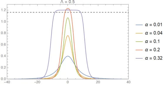
C. Localized solutions and dependence onα 51
E. Extension of the V-K criterion 54
1. a(x) =b(x) 55
2. a(x) =−b(x) 57
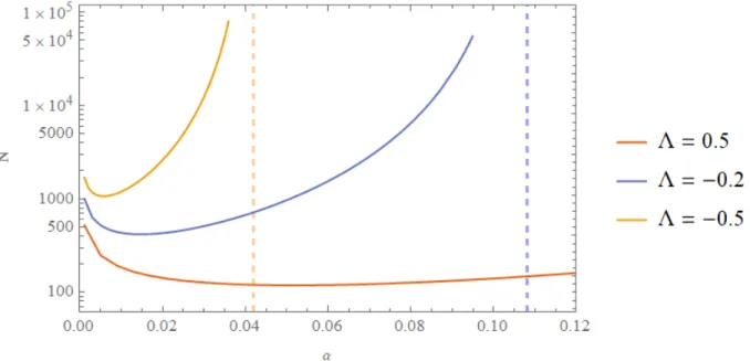
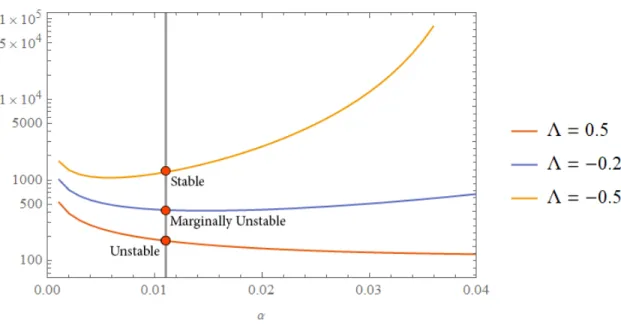
F. Numerical analysis 58
G. Summary and discussion 63
V. General Multi-Field oscillons 65
A. Symmetric potentials with quartic interactions 66
1. m1=m2 67
2. m21−m22 = ∆2· 68
3. m21−m22 = ∆2·2 69
4. Localized solutions 69
5. Numerical stability analysis 70
B. Qualitative discussion and considerations for asymmetric couplings 72
VI. Conclusion and Future Directions 75
VII. Acknowledgements 76
I. INTRODUCTION
What do fundamental particles, atoms and molecules have in common? All of them represent extremely stable configurations containing high concentrations of localized energy. It is therefore obvious that localization of energy is an all-encompassing concept that is fundamental to under-standing the natural world. In fact, in the last 50 years, physicists and mathematicians alike have found a plethora of nonlinear field theories capable of supporting a wide variety of localized structures. The family of such structures that is expected to be most relevant to physics are those that have a stable character. Intuitively this simply means that, once these structures are formed, they will continue to exist for long periods of time. Only when this is the case can we expect that they have a role to play in cosmic history.
Although many of such configurations exist, their characteristics vary quite a bit. In some cases they are completely static, like the Sine-Gordon solitons; while in other cases they oscillate in time, like Q-balls. They can be either stable because the nonlinear potential introduces some sort of conserved charge in the system, or because of specific interactions between nonlinearities in the potential and dispersive effects. In this thesis I will be investigating those objects that are called oscillons. These are oscillating (hence the name) localized structures that can exist in nonlinear scalar field theories if the potential satisfies certain conditions. Since a large plethora of stable and static configurations have been discovered in nonlinear field theories it might now be wise to spend some time outlining the properties of oscillons, what makes them different from other localized structures, and what their relevance might be in the physical world.
A. What are oscillons?
dispersive effects. Oscillons are oscillating (hence the name) and have no known conserved charges.
Examples of solutions falling into other categorizations are Q-balls and Sine-Gordon solitons [1, 2], although a lot more have been found. Q-balls are also oscillating but have a conserved charge that causes them to be stable. The same can be said of Sine-Gordon soliton kinks although they are also completely static. To see how a conserved charge can lead to stable configurations let’s consider a typical Q-ball configuration. Starting from a potential that hasU(1) symmetry
L=|∂µφ|2−U(|φ|) (1) The Q-ball is then defined as a region where the field is not equal to the global minimum ofV(|φ|) (or vacuum) and oscillating with frequency ω: φ = Φ0eiωt. The energy within the region is then simply
E= (ω2Φ20+U(Φ0))V (2)
Where V is the volume of the region. Now, because of the U(1) symmetry of the system there is a conserved charge in the region given by Q =ωΦ20V. Plugging this back in and minimizing the energy with respect to the volume we obtain a new expression forE
E =Q s
2U(Φ0) Φ2
0
(3)
It becomes clear that, sinceQis conserved the Q-ball configuration is stable if 2U(Φ0)
Φ2 0
is minimized by Φ0 6=φvac, since any decay would then be energetically unfavorable. Clearly, conserved charges can cause structures in nature to become stable in this way. What’s interesting about oscillons is that they exist solely due to non-trivial interactions between nonlinearities and dispersion. They do not require any additional symmetries in order to exist which makes them much more general.
B. History
The first indication for the existence of oscillating, localized structures in nonlinear scalar field theories, came in the 70’s [3]. They were initially dubbed pulsons and were found to emerge naturally after bubble collapse in a very constrained nonlinear scalar field model. These findings didn’t gain much traction initially. With the emergence of Cosmology as a data-driven science in the following decades however, and the potential importance of phase transitions and symmetry breaking in the early Universe became apparent, interest in relativistic nonlinear field theories piqued. Solitons became a central theme in scientific debate because of their supposed natural for-mation under cosmological circumstances. This lead to the (re)discovery of a wide range of stable field configurations like Q-balls, Peakons and Solitonic kinks [1, 4, 5]. Eventually it was shown in 1994 that extremely stable, oscillating structures emerge under very general conditions during bubble collapse in nonlinear field theories. These were subsequently named oscillons by the au-thor, M. Gleiser of the original paper. This is where the history of oscillons, albeit short, begins [6].
Although a lot is still unclear about the precise workings of oscillons, steady progress in un-derstanding them has been made in the last twenty years. Initially, most work focused on sim-plistic models, where the oscillon is approximated as a pure Gaussian oscillating harmonically: φosc ∼ e−r
2
cosωt [7, 8]. The whole oscillon profile is essentially reduced to two parameters: its width and its amplitude. These two can then be taken as probes for measuring the degree in which the oscillon ”feels” the nonlinearities in the potential. It was quite clear that these weren’t the real oscillon solutions, since numerical simulations showed that the Gaussian first relaxed into a configuration with a different asymptotic behavior: φ(r)∼e−r asr→ ∞, before reaching stability. However, since the model was simple, one was able to make predictions about the stability and eventual collapse of the oscillon. With this ansatz it was shown that oscillons are present in a wide variety of models. They exist in the Sine-Gordon potential, they electroweak sector of the Standard Model, in the SU(2) gauged Higgs model and all sort of nonlinear scalar field theories [9–11].
were tackled early on using the Gaussian models highlighted above. Numerical and analytical techniques led some scientists to conclude that the oscillon is indeed unique and loosely attractive. However, the simplicity of these models carries an inherent imprecision and rigorous mathematical arguments to tackle these problems are still needed to this day. The issue did inspire the use of a perturbative technique called the two-timing analysis in order to analytically construct the oscillon spatial profile. There now was a way to systematically find an equation, often called the profile equation, that the spatial envelope of the oscillon should solve. The problem of finding oscillons was now reduced to finding zero-mode solutions of this equation which resolved the uniqueness problem somewhat [12].
Application of perturbation theories in this way was an important step in understanding os-cillons. Oscillon solutions could now be constructed, either analytically or numerically, which made it possible to study their stability more precisely. Through the rediscovery of older mathe-matical work, it became apparent that the oscillon solution is merely an asymptotic solution and that it will always lose energy through outgoing radiation. It was shown that this radiating tail was exponentially suppressed however, leading to the first clear mathematical explanation for the longevity of oscillons. It was also shown that this might not be the case for quantum mechanical radiation. Now that the spatial profiles of oscillons were known physicist could assess the stability of oscillons against small perturbations. This can be done by application of Floquet theory, but is in general very complicated. The Vakhitov-Kolokolov criterion has since been used to address specific initial conditions, but the problem has never been solved for generic perturbations [13, 14].
Oscillons in models with multiple interacting fields are more complicated to study [9, 11, 21, 22]. The amount of literature on this topic is therefore somewhat lacking which is a problem since fields in the physical world tend to interact with each other. Oscillons do in fact exist in these multi-component systems, and have even been shown to form in hybrid Inflation models. A better understanding of their properties is needed in the future. The goal of this thesis is to take the first steps in the right direction, outlining where these type of oscillons might differ from single-field oscillons, but also what similarities they share. A lot of research is still needed but in this work are the first indications as to where potential solutions can be found.
C. This Thesis
II. SINGLE-FIELD OSCILLONS
In general it should not be expected that isolated scalar fields exist in nature. Only if a system has very specific symmetries in place, or certain symmetries are broken, it is impossible for (quantum) fields to couple. In all other cases, the general field theoretic approach dictates that all possible couplings between the fields are present. The study of oscillons in these types of isolated systems is therefore most likely a purely mathematical exercise and I aim to study more realistic models in later sections. However, for the uninitiated reader it can be helpful to understand the exact workings of oscillons in these simplified systems. Furthermore, since these type of oscillons are understood relatively well, they might give intuition about the more complicated models I will consider in later sections. So in this chapter we will investigate the world of oscillons in isolated scalar fields. First, we’ll have to understand what conditions the system must satisfy in order to support stable oscillons.
A. Dispersion
In section I it was already mentioned that not all models support oscillons. To illustrate this, let’s consider a free field theory. The potential of such a theory contains no nonlinear terms by definition. The Lagrangian of the field φcan then be written
L= 1 2∂µφ∂
µφ−1 2m
2φ2 (4)
Resulting in an equation of motion that is in fact the Klein Gordon equation
(∂2+m2)φ= 0 (5)
Oscillons, by definition are localized, oscillating configurations in the field that remain stable for timescales that are orders of magnitude bigger than the natural timescales of the system (like the oscillation time). However, any configuration that evolves with equation (5) will tend to spread out over space, a phenomenon probably familiar to the reader as dispersion. Ultimately this is due to the fact that in a free theory all Fourier modes are decoupled and therefore all k-modes travel independently at different speeds during the time evolution of the system. This will delocalize the original configuration. Let’s see how this works in more detail. Switching to Fourier space, equation (5) becomes
¨
Clearly, each Fourier mode evolves independently as a plane waveφk∝ei(kx−ωt), whereω is given by the dispersion relation
ω(k) =pk2+m2 (7)
Let’s now see what happens to an initially localized configuration. We consider a wave-packet in one spatial dimension such that initially
φ(x,0) =e−
1 2
x−x
0
σx
2
(8)
The field is a Gaussian centered aroundx0with widthσx. Fourier transforming this initial condition is straightforward
φ(k,0) = σx 2√πe
−σ2x
2 k 2
eikx0 (9)
Now, using equations (6) and (7) the general solution at some later time can be readily found
φ(x, t) = Z
dk σx 2√πe
−σ2x
2 k 2
eikx0ei(kx−
√
k2+m2t)
(10)
From equation (9) it becomes evident that large k-modes are exponentially suppressed in this approximation. This allows us to Taylor expand the dispersion relation in equation (10) to second order and obtain an exact solution
φ(x, t) = Z
dk σx 2√πe
−σ2x
2 k 2
eikx0ei(kx−m2t−k 2 2mt)
φ(x, t) = exp − 1 2
(x−x0)
q σ2
x−im1t
2 e−im
2t
φ(x, t) = exp "
−1 2
(x−x0) σ(t)
2# eiγ(t)t
(11)
Clearly, the solution remains Gaussian, but now with a time-evolving width
σ(t) =σx
s
1 + 1 m2σ4
x
t2 (12)
And modulated by a phase
γ(t) =−m2t− tm t2+σ4
xm2
(13)
We are mainly interested in the implications of equation (12) which tells us that the solution will spread out over time
σ(t)2−σx2 = t 2 m2σ2
x
So σ(t) → ∞ as t → ∞. The spreading happens over timescales that are comparable to the natural timescales of the theory∼mσx2. So the initial localized packet will spread out and become delocalized.
The argumentation listed above can be generalized to any theory with a clearly defined disper-sion relation forω(k), since we can always just Taylor expand the relation for smallk and obtain similar results. In fact, if there is a clearly defined relation for ω(k) that is not purely linear, the speed of the different k-modesvk = ω(k)k will vary, which makes it impossible for a localized solu-tion to stay exactly that: localized. Clearly, any linear field theory (like the free example discussed above) will have a well-defined dispersion relation. Also, if we’re considering massive relativistic theories the dispersion relation will never be purely linear. From these considerations we conclude that we must look for nonlinear field theories in order to find oscillons. In nonlinear field theories the different k-modes of the field couple in non-trivial ways. There is therefore no clear way to write down a dispersion relation. Simply adding nonlinearities to the theory is not enough however. We’ll explore the relevant conditions in the next section.
B. Restrictions on the nonlinear potential
We are looking for scalar potentials that support localized, oscillating solutions. Oscillons don’t require conserved charges to exist and therefore there are no symmetry restrictions on the potential. A scalar field in an expanding background will evolve with the equation of motion
¨
φ+Hφ˙−∇ 2 a2φ+V
0(φ) = 0 (15)
Where H is the Hubble constant. Plugging in an ansatz for the oscillon solution as φosc = Φ(x) cosωt, equation (15) becomes
−ω2Φ(x)−HωΦ(x) tanωt−∇ 2 a2Φ +
V0(φ)
cosωt = 0 (16)
Since we’re looking for localized solutions of Φ(x), we must have that Φ(x) → ∞ asx → ∞. We can therefore throw away all nonlinear terms
−ω2Φ(x)−HωΦ(x) tanωt− ∇ 2
a2Φ(x) +m
2Φ(x) = 0 (17)
Since this equation should be valid at all times, and a localized solution decays asx→ ∞(leading to the conclusion that ∇2Φ>0 in the asymptotic region), it is straightforward to conclude
Plugging in (18) into equation (16) we obtain
κ2Φ(x)−(Hωtan(ωt) + ∇ 2
a2)Φ(x) +
(V0(φ)−m2Φ cosωt)
cosωt = 0 (19)
Where κ2 = m2−ω2 > 0. Again this should be valid at all times; setting t = 2πω, the equation becomes
κ2Φ(x)− ∇ 2
a2Φ(x) + (V
0(Φ)−m2Φ) = 0 (20)
If smooth localized solutions exist than necessarily there is a region near the center of the solution where ∇a22Φ(x)<0. This imposes a heuristic condition on the potential of the scalar field. Namely,
V0(Φ)−m2Φ<0 (21)
For at least some region of the potential. Furthermore the region should be probed by field values that are of the same order of magnitude as the oscillon itself. Although the most straightforward way to satisfy (21) is to add nonlinear terms to the potential, it has been shown that the same effect can be produced in a system with non-canonical kinetic terms [23].
Many physically motivated potentials that satisfy condition (21) exist. In particular, oscillons have been found in several systems similar to the Standard Model [9, 11]. Furthermore, slow-roll Inflation can be sourced by a scalar field that supports oscillons as well. This idea will be inves-tigated in the next chapter. In the next two sections I will focus on the analytical construction of the oscillon. First, I’ll find the spatial profile of oscillons in a particular scalar field model via a perturbative technique called the two-timing analysis. Then we’ll focus on the asymptotic behavior of this oscillon in the far distance regime, outlining why the oscillon can be so extremely long-lived. The analysis is done for a particular model but the techniques and conclusions can be easily generalized to other systems.
C. Oscillon analytical construction
Let’s consider the action of a scalar field minimally coupled to gravity
Sscalar=
Z
dd+1x√−g[1 2g
µν∂
µφ∂νφ+V(φ)] (22)
With a potential given by
V(φ) = 1 2m
2φ2−1 4λφ
4+1 6gφ
Where m, λ, g > 0 and m, λ, g ∼ O(1). In what follows I will assume the Universe to be static (H = 0) and set a= 1 without loss of generality. Clearly, the potential in (23) satisfies condition (21) for some range ofφ. The sextic term is added to assure that the field remains bounded from below. The equation of motion of the scalar field can be readily obtained by extremizing the action (22). It is
¨
φ− ∇2φ+m2φ−λφ3+gφ5 = 0 (24)
Assuming the field is spherically symmetric
¨
φ−∂r2φ−(d−1)
r ∂rφ+m
2φ−λφ3+gφ5 = 0 (25)
Since equation (25) is nonlinear it isn’t obvious how to find localized field configurations that behave like oscillons. There exists a perturbative approach to this problem however, often referred to as the Two-timing analysis in the literature. The idea is that the oscillon has relevant behavior on two distinct time scales. The technique can be understood intuitively by imagining a completely uniform field oscillating in a purely quadratic potential. The theory is then linear and the field simply oscillates at its natural frequency m. Adding nonlinear terms to the potential as in (23) will alter this frequency, but if the amplitude of the configuration is small, the nonlinearities are only probed perturbatively. Two different time scales can therefore be identified: a short time scale associated with the natural frequency of the system and a long time scale over which the nonlinearities of the potential become significant. Localized, oscillating solutions (oscillons) can therefore be found by perturbatively moving away from a uniform field moving in a quadratic potential. The solution is then also expected to be wide, so that the gradient terms also only enter perturbatively. These considerations inspire the following change of variables
τ =2t (26)
ρ=r (27)
where 1. Here τ is the ”slow” time scale associated with the deviation from the natural frequency andρwith the ”long” spatial width that the oscillon has. Since the oscillon has behavior on both the slow and natural time scales, we sendφ(x, t)→φ(ρ, τ, t). The time derivatives in (25) thus become full derivatives
∂t→dt=∂t+2∂τ
∂t2→d2t =∂t2+ 22∂τ∂t+O(4)
Finally, plugging all of this into the equation of motion in (25) we obtain
∂t2φ+ 22∂τ∂tφ−2∂ρ2φ−2
(d−1)
ρ ∂ρφ+m
2φ−λφ3+gφ5+O(4) = 0 (29)
This is all we need to perturbatively find our oscillon solution. As in standard perturbation theory we introduce an ansatz φ=φ0+φ1+2φ2+...and solve the equations order by order. However, in this case we should not allow for a zero-order term since by assumption the nonlinearities in the potential can only by probed perturbatively in order for the two-timing analysis to be valid. So
φ(ρ, τ, t) =
∞ X
n=1
nφn(ρ, τ, t) (30)
Inserting the expansion in (30) into (29) we can write down the first three order equations O():
∂t2φ1+m2φ1= 0 (31)
O(2):
∂t2φ2+m2φ2= 0 (32)
O(3):
∂2tφ3+m2φ3=−2∂τ∂tφ1+∂ρ2φ1+
(d−1)
ρ ∂ρφ1+λφ 3
1 (33)
The first and second order equations, (31) and (32), are immediately identified as the equations for a harmonic oscillator with massm. It is straightforward to write down a general solution, requiring the result to be real
φ1(ρ, τ, t) = Re{A(ρ, τ)eimt} φ2(ρ, τ, t) = Re{B(ρ, τ)eimt}
(34)
Where A(ρ, τ) and B(ρ, τ) can be imaginary functions. These functions capture the behavior of the solution on long time- and spatial scales, and can thus be thought of as encompassing the oscillon behavior. They are therefore often referred to as the envelope functions of the oscillon in the literature. To find equations governing these envelopes we plug in the solution φ1(ρ, τ, t) = Re{A(ρ, τ)eimt}= Aeimt+A2∗e−imt into equation (33)
∂t2φ3+m2φ3 =
−im∂τA+ 1 2∂
2 ρA+
(d−1) 2ρ ∂ρA+
3 8λ|A|
2A
This is nothing more than the equation of a harmonic oscillator of massmwith a parametric driving force. Notice that the term between brackets is then a resonant term since it oscillates with the natural frequency m. This term will amplify φ3 due to resonance. However, by assumption this can not be the case since the oscillon remains small. The term between brackets has to equate to 0, resulting in the envelope equations of the oscillon
−im∂τA+ 1 2∂
2 ρA+
(d−1) 2ρ ∂ρA+
3 8λ|A|
2A= 0 (36)
Equation (219) is of the Non-linear Schrodinger type and governs the behavior of the oscillon on long time- and spatial scales. Since we’re interested in finding the spatial profiles of the oscillon we perform a separation of variables: A(ρ, τ) =a(ρ)eicτ, wherecis some arbitrary constant and a(ρ) a real function of the spatial profile of the oscillon. Inserting this in the envelope equation gives us the profile equation
−m2a+∂ρ2a+(d−1) ρ ∂ρa+
3 4λa
3 = 0 (37)
Where we set c = −m
2. A few remarks about the parameter c are in order. c is in essence a free parameter, as long as it is not too large. This is simply because it can be absorbed into a redefinition of , since τ =2t. We don’t lose any generality by setting c=−m
2. We also require c <0 for the solutions to decay as a→0 and ρ→ ∞. In this asymptotic regime (221) reduces to ∂ρ2a=−cma, and localized solutions must therefore havec <0.
The oscillon spatial profile are localized solutions of (221). Finding the solutions aloc(ρ) al-lows us to write down the analytical form of the oscillon up to first order in
φoscillon(x, t)≈φ1(x, t) =Re{a(ρ)eim(t− τ
2)}=aloc(x) cos
mt(1− 2 2)
(38)
The frequency of the oscillon is therefore ω = m(1− 2
problem will be tackled in section II D. For now, let’s focus on finding the localized solutions of the profile equation (221).
1. Localized solutions of the profile equation
We managed to reduce the problem of finding oscillons to finding localized solutions of the profile equation (221). This can in some cases be done analytically but will in general require numerical methods. Before we do this, we might want to ask ourselves how many of such solutions exist. Here we focus strictly on the zero-mode solutions, meaning that they are strictly positive (or negative). This is best understood by first examining the one-dimensional case for which d= 1. The profile equation reduces to
−m2a+∂ρ2a+3 4λa
3 = 0 (39)
If we interpret ρ as a temporal instead of spatial variable, equation (39) looks like the equation of motion of a point particle of unit mass, moving in zero-dimensional space under influence of a conservative potentialV(a) =−1
2m
2a2+ 3 16λa
4. The equation therefore has a ”conserved energy”
Eρ= 1 2(∂ρa)
2+V(a) (40)
For localized solutions as ρ → ∞ we have that ∂ρa → 0 and a→ 0. We conclude that localized solutions must have 0 energy. Requiring the solution to be smooth at the origin,∂ρa(0) = 0, and using (40), completely fixes the localized solution of the second order PDE in (39)
V(a(0)) = 0→a(0) = 0∨a(0) =±m r
8
3λ (41)
We conclude that there are exactly two localized solutions of the profile equation in one di-mension, sincea(0) = 0 just gives a(ρ) = 0 everywhere, which is not very interesting. These two solutions satisfya1(ρ) =−a2(ρ). In fact, in one dimension the profile equation can be solved ana-lytically. The solution is a sech function, and for this specific model reads a(ρ) =m
q
8
3λsec(mρ). The situation is a little more tricky in higher dimensions since there is now a friction term in the ”equation of motion” (∝∂ρa) and the energy of the solution is no longer conserved. We can rewrite the profile equation using the energy defined in (40)
dEρ dρ =−
d−1
ρ (∂ρa(ρ))
2 (42)
far-distance regime we conclude thatEρ≥0 atρ= 0. We again require the solution to be smooth at the origin; this puts a bound ona(0)
|a(0)|> m r
8
3λ (43)
So what kind of solutions that satisfy this condition exist, and how many of them are localized (a→0 as ρ→ ∞)? It is best to think about this in terms of the trajectories of solutions in phase space (a, ∂ρa). Since we’re interested in functions that are smooth at the origin, all trajectories start on the ∂ρa = 0 axis. Any trajectory will continuously intersect Eρ = k curves, and due to relation (42), the k-value of these curves must decrease asρ → ∞. The k= 0 curve then defines the boundary between localized and non-localized solutions. Namely, a localized solution must intersect this curve in the origin.
It turns out that only a countable set an(ρ) of these kind of trajectories can be drawn in phase space [24]. Here n is the amount of nodes of the solution. We conclude that there is exactly one zero-mode solution of the profile equation (really two since again−a0(ρ) is also a solution), even in three dimensions. This simply means that for every choice ofthere exists exactly one zero-mode oscillon. However, since the only requirement foris that it is a small number, the model defined in (22) still has an infinite amount of oscillon solutions, all oscillating at frequencies defined by the specific choice of : ω=m(1−2
2). To find the exact spatial profiles ford6= 1 we are restricted to numerical methods. These were found ford= 3 using the shooting method.
2. Scaling dependence of and free parameters
In our quest of finding the profile equations through the two-timing analysis, we’ve implicitly made some assumptions about the scalings of our perturbative approach. To be completely general we should write
τ =δτt ρ=δρr
φ=
∞ X
n=1 δnφφn
FIG. 1: The path in phase space (a, a0) of three different solutions of the profile equations that are smooth at the origin. Once the path intersects theEρ= 0 curve it can never leave the region enclosed by it due to relation (42). A localized solution must intersect this curve in the origin. It
turns out there are a countable set of such solutions.
Where δτ, δρ and δφ are just small numbers. In our derivation we set δτ = 2 and δρ = δφ = ; but there is no a-priori reason to believe that this is the only option. To see why these scalings are correct consider a schematic form of the equation of motion after inserting (44) (in d= 1 for simplicity’s sake)
∂t2φ+ 2δτ∂t∂τφ+δτ2∂2τφ−δ2ρ∂ρ2φ+m2φ+ [nonlinear] = 0 (45) To find well-defined profile equations the slow time scale δτ needs to enter at the same order in perturbation theory as the long space scale δρ. From inspection of (45) we immediately conclude δτ =αδ2ρ, withα∼O(1). Furthermore, to have well defined localized solutions, the first nonlinear term in (45) should also enter at this order. Since in the potential under consideration this is a cubic term we conclude δφ3 = β2δφδρ2, with β2 ∼ O(1), and thus δφ = βδρ. Setting δρ = completely fixes the other scalings up to two free parametersα andβ. To see how the introduction of these parameters influences the oscillon spatial profile, consider the envelope equation under these scalings (in one dimension for simplicity)
−imα∂τA+ 1 2∂
2 ρA+λ
3 8β
Using separation of variables and plugging in A = a(ρ)eicτ = a(ρ)eicα2t, gives us the modified profile equation of the oscillon
2mαca(ρ) +∂ρ2a(ρ) +λ3 4β
2a(ρ)3= 0 (47)
Naively, We must conclude that for each choice of the the small parameter, which fixes the width of the oscillon through the parameter ρ, there is a family of profile equations, all with different zero-mode solutions, that when solved might yield stable oscillons. However, this is in fact not true, and these are ”phantom” parameters. To see this suppose we have a solutiona1(ρ) for specific choices β1 and κ1 = αc. Let’s now suppose we’re looking for a solution a2(ρ) corresponding to choicesβ2 and κ2. This solution should off course solve
2mκ2a2(ρ) +∂ρ2a2(ρ) +λ 3 4β
2
2a2(ρ)3= 0 (48)
Then plugging in the ansatz solutiona2(ρ) =Ba1(Aρ), we obtain (after some rewriting)
2mκ2
A2a2(Aρ) +∂ 2
Aρa1(Aρ) + B2 A2λ
3 4β
2
2a1(Aρ)3= 0 (49) So we reach the conclusion that A = pκ2/κ1 and B = ββ12
p
κ2/κ1. So how does the oscillon solution look like in real space for the choices β2 and κ2. Using the solution we found for a2(ρ) and (38)
φosc(x, t) =β1
p
κ2/κ1a1(
p
κ2/κ1x) cos (m+κ22)t
(50)
Now it becomes evident that the actual oscillon solution is exactly the same as the solution we found for parameters β1 and κ1, just for a different. Namely, write ˜=
p
κ2/κ1to obtain
φosc(x, t) = ˜β1a1(˜x) cos (m+κ1˜2)t
(51)
The two-timing analysis reduces the problem of finding oscillon solutions to that of finding zero-mode solutions of the profile equation. The amount of free parameters might differ between zero-models, but the technique remains robust in general. It is in essence a special application of perturbation theory, which means that to any order solutions can only be asymptotically correct. Since oscillons have been observed to be extremely long lived, the corrections to the perturbative expansion can not be too large. In fact, in the next section we’ll see that they produce outgoing radiation that is exponentially suppressed.
D. Radiation
The two-timing analysis highlighted in the previous section is a clear-cut procedure that allows one to find localized oscillating solutions of a given theory. One simply chooses a small scaling parameter and solve the equations of motion perturbatively. Spatial profiles are then found by requiring that resonant terms cancel at each order, resulting in the so-called profile equations from the previous section. It was understood quite early on by mathematicians that this procedure will in general not converge to a perfect breather solution [25]. Breathers are localized oscillating solutions of a nonlinear theory [26? ]. It misses an exponentially small radiating tail∼e−1 that is beyond all orders in perturbation theory. An important exception is the Sine-Gordon breather. In recent years physicists realized that this principle should also apply to oscillons, and it was shown that in fact they lose energy via radiation. In this section we’ll see why the oscillon solution must in fact have a small radiating tail, and how to find it.
The fact that (most) oscillons have a radiating tail is ultimately tied to the fact that the se-ries expansion in is only asymptotically correct. To any order in perturbation theory the series expansion will not exactly solve the equation of motion: there will always be a remainder term that acts as a source for radiation. To see this, consider a scalar field theory with potential
V(φ) = 1 2φ
2−1 4φ
4+ 1 6φ
6 (52)
Clearly this potential satisfies condition (21) and this theory supports oscillons. It is just the theory considered in the previous section, with all couplings set to 1.
¨
Now consider the oscillon solution truncated to order N
φ(x, t) = N
X
n=1
nφn(x, t) (54)
where all individual φn are found by perturbatively solving the equation of motion as explained in the previous section. At each order the equation of motion is a (forced) harmonic oscillator equation of which the solution can be found exactly. Eachφn can therefore be written in the form φn∼a(ρ) cos(nωt) +...whereω= 1−
2
2 andn= 1,3,5 since the potential is symmetric. Plugging this solution into the equation of motion it is clear that all terms up to∼O() cancel. Furthermore, all terms proportional to cos(ωt) also cancel by construction. However, there now clearly remain terms that are of higher order inand don’t oscillate at frequencyω. In this specific potential the remainder term can schematically be written as
J(x, t) =N+2j(x)cos(3ωt) +h.h.+O(N+3) (55)
which will in general not be 0 (albeit very small). The only way to solve this discrepancy is to add a perturbation to the oscillon solution. Writingφ(x, t) =φosc+δ(x, t) and linearizing the equation of motion we see thatJ(x, t) acts as a source
¨
δ− ∇2δ+δ =J(x, t) (56)
Where I’ve ignored a parametric resonance term∝Vφφ(φosc)δthat is suppressed relative toJ(x, t). The remainder of the asymptotic oscillon expansion thus sources a perturbation and we’ll see that this results in outgoing radiation. The full derivation involves complex analysis and some readers might satisfy themselves with the hand-wavy argumentation presented here. All they should know is that the solution of δ(x, t) is exponentially small δ(x, t) ∼ e−1 making oscillons extremely long-lived. In what follows I present a more nuanced analysis[27–29].
The perturbative expansion of the field φ(x, t) =P
are given by
φ1 =f1(x) cos(ωt)
φ3 =f3(x) cos(ωt) +F(x) cos(3ωt)
φ5 =f5(x) cos(ωt) +G(x) cos(3ωt) +H(x) cos(5ωt)
(57)
Where allfn can be found by cancelling resonant terms and the functionsF, G, H... can be found by solving the forced harmonic oscillator equations at each order
F(x) = 1 32f
3 1 G(x) = 1
8
3 4f
2 1f3−
5 16f 5 1 + 6 128f 5 1
H(x) = 1 24 3 128f 5 1 − 1 16f 5 1 (58)
All φn in the peturbative expansion are time-periodic in ω; and all spatial functions in (58) are uniquely defined. It is therefore natural to search for a solution in terms of Fourier modes and use the functions in (58) as boundary conditions near the central part of the oscillon. We look for solutions
φ(x, t) =
∞ X
n=0
Φn(x) cos(nωt) (59)
Plugging these into the equations of motion and gathering terms oscillating at the same frequency, we obtain equations for the spatial part of the Fourier modes (working in d = 1 and assuming spherical symmetry)
−n2ω2Φn−∂r2Φn+ Φn=Fn (60)
Where Fn is a nonlinear function of the (other) Fourier modes. In a symmetric potential Fn = 0 for evennand there are no localized solutions for the corresponding modes. The small amplitude expansion actually gives expressions for the different Fourier modes.
Φ1=f1+3f3+5f5+... Φ3=3F +5G+... Φ5=5H+....
(61)
We’ve seen that with the potential in (52), f1(x) =
q
8
3sech(r). We can analytically con-tinue this function to the complex plane. Here the sec function has a pole at x = iπ2. Sim-ilarly there is one at x = −iπ
2. The sech-function can be expanded around its upper pole sech x=R+ iπ2 =−Ri +iR6 +O(R3) for small |R|. The Laurent series around the upper pole of f1(x) can then be written as
f1(y) =−
r 8 3
i y+i
r 8 3
y 6 +O(
3y3) (62)
WhereR=y=r−iπ2. The matching region is defined asy → ∞. For R to remain small we also send → 0. From (61) we learn that to lowest order in the Fourier modes Φn are proportional tonf1n. In the matching region they satisfy
Φ1=−
r 8 3 i y +O(
2,1/y2)
Φ3= 8 3 r 8 3 i
y3 +O(
2,1/y4)
Φ5=− 64 9 r 8 3 i
y5 +O(
2,1/y6)
(63)
In the matching region the mode-equations (60) can be written as
−n2Φn−∂y2Φn+ Φn=Fn (64)
We need to find solutions of (64) that can be matched upon the boundary conditions in (63). The asymptotic expansion converges nowhere and it is not clear how to find a correction to the series. Notice however that for Re(y) = 0 the imaginary part of the series converges trivially; namely Im(Φn) = 0. In order to find a correction to the series that satisfies this condition we split the modes into real and imaginary parts Φn= Ψn+iΩn. Plugging this into (64)
−n2Ωn−∂y2Ωn+ Ωn= Im(Fn) (65)
In the matching region we see that all Φn → 0 and we can approximate the solution by ignoring the nonlinear terms ∝Fn. To first order the solutions are then
Ω1 =ν1y Ω3 =ν3exp
−i √
8y
Ω5 =ν5exp
It becomes clear that only the solutions for n≥3 can be matched to the expansion on the real axis as Im(y) → −∞. Switching back to the coordinate y = r− iπ
2 we find corrections of the expansion beyond all orders
δΦ1= 0 δΦ3=iν3exp
−i√8r
exp
−√8π 2
δΦ5=iν5exp
−i√24rexp−√24π 2
(67)
So that the correction to the real part of the expansion is δΦ1 = 0
δΦ3 =ν3sin
√
8rexp−√8π 2
δΦ5 =ν5sin
√
24r
exp
−√24π 2
(68)
Since these corrections are exponentially suppressed we can approximate the full oscillon solution as a superposition of these corrections and the standardexpansion. We get a final expression for the oscillon
φosc=
X
n=1
nφn+ν3sin
√
8rexp−√8π 2
cos(3ωt) +h.h. (69)
The corrections will only dominate the solution asr → ∞since in this regime allφn→0. We can then obtain an approximate expression for the radiation tail of the oscillon
φrad ≈
X
n=3 νnsin
p
n2−1r+nt) exp−pn2−1π 2
(70)
Where the sum only runs over odd n. Since the radiation tail is suppressed, the energy loss in the oscillon is extremely slow. Since the energy in the radiation is proportional to the squared amplitude of the tail, it becomes clear that
dE dt ∝exp
−pn2−1π
(71)
E. Linear Stability Analysis
In the previous sections we’ve constructed oscillon solutions perturbatively using the two-timing analysis. These solutions lose energy via a small radiating tail that will dominate the solution in the far-distance regime. The rate of energy loss is very small however, which results in an extremely long-lived oscillon. In this section we’ll be interested in the behavior of small perturbations living atop the ’core’ part of the oscillon, which means we won’t be interested in the small radiating tail. The main question we would like to answer is what conditions an oscillon should satisfy in order to be stable against small perturbations. This is an important question since it is expected that perturbations arise naturally, both through radiation and coupling to other fields. If the oscillon is not robust to such perturbations, it might decay rapidly.
To analyse the stability of oscillon solutions we again work in a scalar field model with potential
V(φ) = 1 2φ
2−1 4φ
4+ 1 6φ
6 (72)
Resulting in equations of motion
¨
φ− ∇2φ+φ−φ3+φ5 = 0 (73)
Although the analysis performed in this section can easily be extended to other models supporting oscillons. In a first step we perturb the field around the oscillon solutionφosc∼a(r) cos(ωt) found via the two-timing analysis
φ(x, t) =φosc(x, t) +δ(x, t) (74)
We assume that the field δ(x, t) is small. Plugging this ansatz into the equation of motion and linearizing the result we obtain the equation thatδ(x, t) satisfies
¨
δ− ∇2δ+δ−3φ2
oscδ+ 5φ4oscδ = 0 (75)
made by separating the analysis for perturbations in two categories. On the one side we analyse perturbations of very short wavelengths (relative to the oscillon), while on the other side we analyse perturbations that are about the same size as the oscillons. For short wavelengths the oscillon only varies very slowly with respect to the perturbation itself. Near the center of the oscillon we can approximate the oscillon as a constant oscillating background. The equation of motion (75) can then be solved in Fourier space using Floquet theory. Perturbations that are about the same size of the oscillon can be analysed using a criterion discovered by mathematicians in the 70’s, called the Vakhitov-Kolokolov criterion. Both analyses will be performed separately.
1. Short Wavelengths: Floquet theory
The two-timing analysis automatically gives oscillons that are quite wide via the introduction of the variableρ=r. The width of the oscillon is thus ofO(1/) in real space, meaning that in Fourier space it has a width ofO() (sincek∝λ−1). When speaking of short wavelength perturbations we mean those k-modes for which k . These modes don’t ”feel” the large scale spatial variation of the oscillon solution and it can therefore be approximated as a constant oscillating background. For perturbations living near the center of the oscillon we writeφosc as
φosc(x, t) =a(0) cos(ωt) =a0cos(ωt) (76)
In this approximation the oscillon has no complicated spatial structure, and there is nothing stop-ping us from analysing the problem in Fourier space. Plugging in the approximation (76) into the equation of motion (75) and switching to Fourier space we obtain
¨ δk+
1 +k2−32a20cos(ωt)2+ 54a40cos(ωt)4δk= 0 (77)
SettingA(t) = 1 +k2−32a20cos(ωt)2+ 54a40cos(ωt)4, equation (77) becomes ¨
δk+A(t)δk = 0 (78)
Now clearly the functionA(t) is periodic. Namely,A(t+2πω) =A(t). Equation (78) is a particular formulation of what is known as ”Hill’s equation”, named after mathematician George Hill, who introduced it in 1886. The equation can be solved using Floquet theory. Setx1=δk and x2 = ˙δk, then equation (78) can be written in matrix form
˙
Where x= x1 x2
, A(t) =
0 1
−A(t) 0
(80)
Floquet theory can be applied to systems which satisfy equation of the form (79) when A is periodic, which clearly is the case here. Floquet theory then tells us that the solutions ofx are of the formx∝eµtp(t) wherep(t) is a periodic function with the same period asA(t). µis referred to as the Floquet exponent and controls whether the solution grows or oscillates. This prompts us to seach for solutions of the form
δk=
∞ X
n=0
cn(t) cos(nωt) +bn(t) sin(nωt) (81)
Where it is assumed that the functioncn(t) and bn(t) are slowly varying with respect to the period T ∼ 2π
ω since the solutions of (77) are purely oscillatory for → 0. To solve this system using Floquet theory we rewrite equation (77)
¨
δk+ Ω2k+2(βcos(2ωt) +γcos(4ωt)
δk= 0 (82)
Where
Ω2k= 1 +k2−2(3 2a
2 0+2
15 8 a
4 0) β =−3
2a 2 0+2
5 2a
4 0 γ =25
8a 4 0
(83)
The Floquet exponent for this set of equations system was found approximately in [18] in the context of oscillon formation during preheating. The derivation of the solution will be given precisely in the next chapter, when we discuss the role of oscillons in cosmic history. For now, the reader must content himself with simply the result:
µk=± 1 4ω
q
β2−4(ω2−Ω2
k)2 (84)
In the region in phase-space (a0, k) where the Floquet exponentµk is real perturbations will grow, and have a chance of destroying the oscillon. Thus we want to find the region where
β2−4(ω2−Ω2k)2 >0∧k (85)
2. Long Wavelengths: the V-K criterion
Applying Floquet theory to perturbations that live on the same spatial scale as the oscillon is a lot more complicated since we now have to consider the spatial structure of the oscillating background. This can in general not be done analytically. Luckily, Vakhitov and Kolokolov de-veloped a clever way to assess the stability of localized configurations in nonlinear field theories. This criterion was later extended to assess the stability of oscillons to exactly these type of large scale perturbations. In what follows I will show how to apply the V-K criterion in this context, and how to derive it exactly.
Since we’re interested in perturbations that are about the same width as the oscillon itself, we again switch variables
r→ρ=r (86)
Assuming that the perturbationδ(x, t) is spherically symmetric and plugging in the oscillon solution φosc(x, t) =a(x) cos(ωt), the equation of motion (75) becomes
¨
δ−2∂ρ2δ−2d−1
r ∂ρδ+δ−3
2a2cos(ωt)2
δ+O(4) = 0 (87)
Where ω = 1 +κ2 (since m = 1 in this specific theory). Remember that κ is a free parameter of O(1) that is negative and enters during the two-timing analysis. Since the perturbations are small. Now, intuitively it is expected that the perturbation will have behavior on two time scales. On the one hand it will oscillate with the oscillon on time scales of order 1/ω while it might also start to grow slowly. This is analogous to the two time scales found in the two-timing analysis and prompts the introduction of two new variables
T =ωt τ =2t
(88)
So in the equations of motion we must change∂t→dtand therefore∂t2 →ω2∂T2+22ω∂T∂τ+4∂τ2 = ∂2
T +2∂τ∂T + 2κ2∂T2 +O(4). Finally we have ∂T2δ+2∂τ∂Tδ+ 2κ2∂T2δ−2∂ρ2δ−2
d−1
r ∂ρδ+δ−3
2a2cos(T)2
δ+O(4) = 0 (89)
order by order. So we write
χ=δ0+δ1+.... (90)
The zeroth and second order equation then become respectively
∂T2δ0+δ0 = 0 (91)
∂T2δ2+δ2=−
∂T∂τ−∂ρ2− d−1
ρ ∂ρ−3a
2cos(T)2
+ 2κ∂T2
δ0 (92)
The most general solution of the zeroth order equation can be written as
δ0(T, τ, ρ) =u(ρ, τ) cos(T) +v(ρ, τ) sin(T) (93)
As expected the perturbation oscillates with the oscillon itself at frequency ω. The potential growth of the perturbations is entirely encoded in the functions u(τ, ρ) andv(τ, ρ). The question is thus there are solutions for u(τ, ρ) and v(τ, ρ) that grow on timescales ∼ τ. By assumption, the perturbation δ(x, t) is small, and there can therefore be no resonant terms at each order in perturbation. Plugging in (93) into (92) and gathering secular terms on the right hand side
∂T2δ2+δ2 =−
∂τv−∂ρ2u− d−1
ρ ∂ρu− 9 4a
2−2κu
cos(T)
+
∂τu+∂ρ2v+ d−1
ρ ∂ρv+ 3 4a
2v+ 2κv
sin(T) +h.h.
(94)
And cancelling the secular terms gives us two linear equations for u(τ, ρ) and v(τ, ρ)
∂τu=−Lv (95)
∂τv=M u (96)
Where L = ∂ρ2+ d−ρ1∂ρ+ 34a2 + 2κ and M = ∂ρ2+d−ρ1∂ρ+ 9 4a
2+ 2κ are linear operators. Since these equations are linear we can perform a separation of variables and writeu(τ, ρ) =u(ρ)eΩτ and v(τ, ρ) =v(ρ)eΩτ. With this assumption equations (95) and (96) reduce to one ”master” equation
−Ω2u=LM u (97)
be real; the perturbation will grow and eventually force the oscillon away from its stable configu-ration. The Vakhitov-Kolokolov criterion can tell us if max(Ω2)>0. I will derive it in what follows.
To find the smallest eigenvalue of LM we would like to invert the operator L. Notice how-ever that L acting on the oscillon spatial profile function a(ρ) is actually nothing more than the profile equation itself. The functiona(ρ) is an eigenvector ofLwith eigenvalue 0. This means that L can not be inverted in the full vector space. However, from (95) and (96) it follows that
Ωhu|ai=h−Lv|ai=− hv|Lai= 0 (98)
Where I’ve made use of the fact thatL is a real operator. Since we’re interested in functionsu(ρ) for which Ω 6= 0, it is sufficient to consider the subspace of functions that is orthogonal to a(ρ). Since a(ρ) is non-vanishing L is non-negative and has exactly one eigenvector with eigenvalue 0, namely a(ρ). This means that on the subspace orthogonal to this function L is positive definite and we can rewrite (97) as
−Ω2= hu|M|ui
hu|L−1|ui (99) So we need to find out if there is a functionu(ρ) orthogonal to a(ρ) for which the right hand side (99) is negative. In particular, since L−1 is positive definite, this is the case when
G= min(hu|M|ui)<0 (100)
So all we need to do is to check this condition on G. To find G we use the method of indefinite Lagrange multipliers. Namely, if we write
M|ui=λ|ui+α|ai (101)
Then G is the smallest value ofλfor which there exists a functionu(ρ) orthogonal toa(ρ) and anα such that (101) is solved. To find the exact value of this particularλone would need to check this for a complete set of functions u(ρ). However we are only interested in the sign of λ. Expanding |uiand|aiin a complete set of orthogonal eigenfunctions|ψni(with corresponding eigenvaluesλn) of M, we obtain an expression for |ui
|ui=α
∞ X
n=1 cn λn−λ
|ψni (102)
Wherecn=hψn|ai. However, since we requireha|ui= 0 and ha|=cnhψn|, we must also have
α
∞ X
n=1 c2n λn−λ
So either α = 0 or f(λ) = 0. From numeric investigations it turns out that M has exactly one negative eigenvalue and that the corresponding eigenvector is non-vanishing. Since forα = 0, the functionu(ρ) is an eigenfunction ofM and sincea(ρ) is also non-vanishing we conclude thatλ≥0 in order for hu|ai = 0. The situation where α 6= 0 might therefore be a bit more interesting. In this casesλis determined by the smallest root of the equation
f(λ) =
∞ X
n=1 c2n λn−λ
= 0 (104)
Since we just concluded that c1 6= 0 corresponding to the only eigenvalue for which λn < 0, we conclude that the smallest root must lie between λ1 < λmin < λ2. Since the function f(λ) only increases between these two values ofλ, it suffices to know the value atλ= 0 in order the know if the smallest root of f(λ) is negative. In particular, if f(0)>0 then λmin <0. We can then write
f(0) =
∞ X
n=1 c2n λn
=
∞ X
n=1
ha|ψni hψn|ai hψn|M|ψni
=ha|M−1|ai (105)
So we are essentially interested in sgn(ha|M−1|ai). To find this let’s derive the full profile equation with respect to the free parameterκ. So
∂La
∂κ = 0 =M ∂a
∂κ+ 2a (106)
Thus we conclude thatM−1|ai=−1 2
∂a
∂κ. PLugging this into equation (105) and rewriting we come to the conclusion
ha|M−1|ai=−1 2 a ∂a ∂κ =−1
4 ∂
∂κha|ai (107)
Finally we have derived the illustrious Vakhitov-Kolokolov criterion
G=−sgn∂I
∂κ (108)
Where I =R dρda(ρ)2 is the definition of the inner product in our vector space. In particular, if G <0, there are perturbative modes of about the same size as the oscillon that will grow and force the field configuration away from the oscillon solution.
perspective, this simply means that κ controls the effective mass of the particles in the oscillon. Since κ must be negative for oscillons, this also explains why oscillons are stable under the V-K criterion: the particles in the oscillon can lower their mass by becoming part of it. Therefore the criterion tells us that, if the oscillon loses particles (approximately governed by I) by decreasing the mass of the individual particles, the solution will be unstable. The individual particles will tend to decrease their own effective mass, which decreases the total amount of particles in the oscillon. The oscillon decays thus decays. Off course, this explanation isn’t perfect, it is just meant to give some intuition about the interpretation of the criterion.
F. Summary
III. OSCILLONS IN THE PHYSICAL WORLD
The reader should at this point have a solid grasp of (single-component) oscillons. Namely, how to construct them, under what conditions they are stable and why they are so extremely long-lived. The reader would at this point be excused in thinking that oscillons are nothing more than mathematical oddities, arising as non-trivial solutions of nonlinear PDE’s. Although it has been shown that oscillons are supported in certain sections of the Standard Model, and it is a real possibility that the Inflaton supports oscillons as well, there is no a priori reason to assume that there are natural processes that create them. At this point it is therefore not at all clear if they have a role to play in cosmic history.
Since this thesis is being written in the context of Physics and not Mathematics it might be wise to spend some time outlining the role of oscillons in the physical world. Namely, during what processes they are formed and what empirical imprints they might leave behind. While much work has been done in this regard, the most interesting claims come from their potential formation during the parametric resonance phase of (p)reheating. In fact, (Slow-Roll) Inflation is one of the most famous examples where nonlinear scalar field dynamics play an important role (together with the Higgs mechanism of course). It is therefore to be expected that oscillons are an eminent figure during this period. In this chapter I will mainly focus on this period, briefly outlining some other cases where oscillons become important in later sections. It will now be useful to shortly recap what Slow-Roll Inflation and (p)reheating entail exactly.
A. Slow-Roll Inflation
the curvature of the Universe to such an extent that the initial conditions of the Universe become in fact irrelevant to the late time observation of cosmological curvature. Finally, the monopole problem highlights the contradiction between the theoretical formation of magnetic monopoles at some GUT-scale and the lack of observation of such particles. Accelerated expansion in the early Universe would dilute these particles, making it nearly impossible to detect them in our time. Besides the resolution of these problems, Inflation also offers a natural way to introduce scalar (and tensor) perturbations in the hot Big Bang model. I will not go further into explaining the appeal of Inflation here and instead refer the reader to the many pages of literature dedicated to this topic.
Although many theoretical models exist that explain how an era of accelerated expansion could occur in the early Universe, I will focus here on the simplest one. This model, referred to as Slow-roll Inflation, involves a single scalar field, called the Inflaton, that is minimally coupled to Gravity. The action is given by
S = Z
d4x√−g[1 2R+
1 2g
µν∂
µφ∂νφ+V(φ)] (109)
Assuming a FRW background geometry and an homogeneous scalar field, the dynamics of the system are given by the Friedmann equation
H2 = 1 3
1 2 ˙
φ2+V(φ)
(110)
and the equation of motion of the scalar field
¨
φ+ 3Hφ˙+Vφ(φ) = 0 (111)
Finally, the energy momentum tensor, defined as δSδφ shows that the scalar field behaves as a perfect fluid with
ρφ= 1 2 ˙
φ2+V(φ) (112)
Pφ= 1 2 ˙
φ2−V(φ) (113)
It is now important to realize that all of the above equations are very general statements about homogeneous scalar fields in a FRW geometry. We will need certain restrictions on our potential in order to cause a period of accelerated expansion. Namely, the acceleration equation in this system becomes
¨ a a =−
1
In order to have a period of accelerated expansion, the right hand side of this equation needs to be positive and we therefore require
ρφ Pρ
= 1 2φ˙
2+V(φ) 1
2φ˙2−V(φ)
>−3 (115)
From (115) we obtain a heuristic argument for Slow-roll Inflation: if there is a region of the potential that is shallow, so that the scalar field kinetic energy is small and the potential energy dominates, equation (115) will always be satisfied. The field is than ”slowly rolling” towards the potential minimum. In this case, where ˙φV(φ), the Hubble parameter given by equation (110) becomes approximately constant
H2 ≈ 1
3V(φ) (116)
Such that the expansion of the Universe is quasi-exponential
a(t)∼eHt (117)
And H is slowly varying. The fact that the accelerated expansion of the Universe needs to persist for a certain amount of e-folds in order to solve the aforementioned empirical problems puts even more heuristic restrictions on the Inflaton potential. These restrictions are summarized in the slow-roll parameters
V = Mpl2
2
Vφ V
2
(118)
ηV =Mpl2
Vφφ
V 2
(119)
Where subscripts signify derivatives with respect toφ. In the region of the potential where slow-roll inflation occurs we must then have
V,|ηV| 1 (120)
FIG. 2: The slow-roll Inflation scenario: the scalar Inflaton slowly rolls down a potential hill sourcing accelerated expansion. As the field reaches its minimum, it starts to oscillate and
deposit energy into other fields. This is the start of reheating.
governed by Quantum Mechanics), the scalar field loses homogeneity and starts to ”fragment”. This stage in cosmic history, referred to as (p)reheating, is the birthplace of the particles of the Standard Model and the start of the Hot Big Bang. In the next sections we’ll see that if the Inflaton supports oscillons, we should expect a significant amount of energy to be frozen in the form of oscillons as well.
B. Reheating
As the Inflaton slowly rolls down the potential, sourcing accelerated expansion of the Universe, there will be a point where the conditions (120) are no longer met and Inflation stops. The Inflaton φthen starts to oscillate around some global or local minimum of the potentialV(φ). The Inflaton φthen satisfies approximately
φ(t) =φ0+ Φ(t) cos(ωt) (121)
Universe evolves as if it was matter dominated. The Hot Big Bang model requires thermal initial conditions however. In standard Inflationary lore this happens through coupling of the Inflaton to gravity and other (Standard Model) fields [30]. This can be modelled approximately by adding an extra friction term to the equation of motion of the scalar Inflaton
¨
φ+Hφ˙+ Γ ˙φ+Vφ(φ) = 0 (122)
Where Γ is the decay rate of the Inflaton into other fields. This equation can be interpreted as follows: the Inflaton loses energy both through coupling to other fields (through Γ) and through expansion (throughH). Since expansion slows down as the Universe expands (we’re in an matter dominated phase), there will be a moment in time where Γ =H. This fixes the temperature scale at which the Hot Big Bang start, since most energy in the Inflaton will decay into particles after this moment in time.
In general, using equation (122) will not give very accurate results. In particular, it neglects fluctuations in both the Inflaton and the metric. Furthermore, finding the decay rate of the Infla-ton through the creation of particles from some vacuum state requires a full quantum mechanical calculation. Both of these points lead to an inhomogeneous decay of the Inflaton where particles and fluctuations are created locally. This epoch of ”local” decay is referred to as preheating. Only after interactions between the locally created particles, does the Universe thermalize. In what follows I’ll show how fluctuations in the field can be enhanced during preheating, forming oscillons.
C. Oscillon Formation During Preheating
As the Inflaton oscillates at the bottom of its potential during preheating it can excite fluctu-ations that eventually become oscillons. To analyse this process we approximate the Inflaton as a homogeneous background field. For oscillons to form the Inflaton potential should satisfy condition (21). Near the vacuum of the field we therefore approximate it as
V(φ) = 1 2m
2φ2−λ 4φ
4+g 6φ
6 (123)
Where we follow the analysis in [18] and [17] by choosingλ, m ∼O(1) and g 1. The equation of motion of the background oscillating field ¯φis then given by
¨ ¯
We can find an approximate solution for the homogeneous oscillating background if we assume the field to be small. Looking at our ansatz in (121) we see that the energy density of the background scales withV( ¯Φ(t))≈ 12m2Φ(t)¯ 2. Since the background is effectively in a matter-phase we conclude
¯
Φ(t) = √Φi¯
a(t)3. This allows us to write down an approximate form for our background oscillating
Inflaton
¯
φ(t) = pΦ¯i
a(t)3 cos(ωt) (125)
Furthermore
H = pHi
a(t)3 (126)
Since we’re in a matter-dominated epoch. Since the background fieldΦ(t) is small by assumption¯ we can plug inΦ(t) =¯ Φ0(t) (where1) into (124) and conclude concludeω2 =m2−2(3λ4 Φ20+ κ58Φ40) +O(3). Here I’ve used the fact that g 1 and set g = κ2. The question now is how
fluctuations of the field are amplified in this oscillating background. The analysis is closely related to the linear stability analysis performed in the last chapter where a key difference is that we are now dealing with a homogeneous background. Adding a fluctuation atop of the background field
¯
φ(t)→φ(t) +¯ δφ(x, t). The equations of motion forδφ(x, t) then are
¨ δφ−∇
2
a2 δφ+ 3Hδφ˙ +Vφφ( ¯φ)δφ= 0 (127) Since this equation is linearized we can best switch to Fourier space
¨ δφk+
k2
a2δφk+ 3Hδφ˙k+Vφφ( ¯φ)δφk= 0 (128) Finding the solutions for the different modesδφkcan thus be done using Floquet theory. We’ll first solve the problem in a static background (H = 0 anda= 1) and extend the solution to understand the behavior in an expanding background afterwards. In a static background
¨
δφk+k2δφk+Vφφ( ¯φ)δφk= 0 (129)
If the background is static the Inflaton oscillates as
¯
φ≈Φ0cos(ωt) (130)
Whereω2 ≈m2−2(3λ4 Φ20+κ58Φ40). We thus need to solve the following equation ¨
Where again I’ve set g = κ2. This equation can clearly be solved using Floquet theory. An
approximate solution for the Floquet exponents of this equation will be found in the next section. These define instability bands in which fluctuations will grow (and maybe even form oscillons). A final remark regarding equation (127) is now in order. A complete analysis of the growth of fluctuations should also consider fluctuations in the metric∼δgµν. This will add an extra term to the equation of motion. We choose here to focus solely on growth through parametric resonance of the background field and ignore these extra terms. Some interesting work regarding the effect of metric fluctuations during preheating has been done in [31, 32].
1. Finding instability bands: Floquet again
Finding the instability bands of equation (131) can be done using Floquet theory. In fact, it can be rewritten into equation (132), and thus has similar solutions for the Floquet exponents. We are now not limited by the assumption thatk, so that fluctuations can grow on all scales. We will now see how to find the exact form of the Floquet exponents µk. We rewrite the equation in (131) as we did before in chapter II. It becomes
¨
δφk+ Ω2k+2(βcos(2ωt) +γcos(4ωt)
δφk= 0 (132)
Where
Ω2k=m2+k2−2(λ3 2a
2 0+κ
15 8 a
4 0) β =−λ3
2a 2 0+κ
5 2a
4 0 γ =κ5
8a 4 0
(133)
In [18] the instability bands were found by looking for solutions of the form
δφk=
X
n=1,2,3
an(t) cos(Ωkt) +bn(t) sin(Ωkt) (134)
˙
x= 1
4ωA·x+O(
2) (135)
Where x= a1 b2
, A=
0 β+ 2(ω2−Ω2k) −β+ 2(ω2−Ω2k) 0
(136)
A has an infinite period (it is constant). This tells us that the solutions of this equation are given byx=eµktp where pis a constant vector. Inserting this into equation (135) we obtain the
following expression
µkx= 1
4ωAx (137)
We conclude that the Floquet exponents are simply the eigenvalues of the matrix 4ω1 A!. They are now readily found to be
µk=± 1 4ω
q
β2−4(ω2−Ω2
k)2 (138)
Finally we obtain an analytic expression for the (growing) Floquet exponent to lowest order in
µk= k 2 v u u t 3λ 2 ¯ φ m 2 1− ¯ φ φi 2! − k m 2 (139)
Where I’ve set ¯φ = Φ0 and φi =
q
3λ
5g. When the expression in (139) is real, modes will be amplified. Using it we can find instability bands in thek−φ¯plane. In a static background modes will forever stay inside the instability bands and grow until they become nonlinear. However the situation is a bit more complex during preheating. In fact during preheating the Universe continues to expand, which we’ve ignored so fat. Both the physical length scale of a perturbation and the amplitude of the Inflaton change. Co-moving modes can therefore enter and an instability band, get amplified for some time, and stop growing once it exits the band again. We’ll now see how amplification works in an expanding background.
2. Including expansion