TREE-BASED METHODS FOR SURVIVAL ANALYSIS AND HIGH-DIMENSIONAL DATA
Ruoqing Zhu
A dissertation submitted to the faculty of the University of North Carolina at Chapel Hill in partial fulfillment of the requirements for the degree of Doctor of Philosophy in the Department of Biostatistics.
Chapel Hill 2013
Approved by:
Dr. Michael R. Kosorok Dr. Jianwen Cai
c ⃝ 2013 Ruoqing Zhu
Abstract
RUOQING ZHU: Tree-based methods for survival analysis and high-dimensional data
(Under the direction of Dr. Michael R. Kosorok)
I dedicate this dissertation work to my parents,
Dr. Lixing Zhu and Qiushi Tian,
who have loved and supported me throughout my life,
and to my beloved wife,
Xian Cao,
Acknowledgments
My graduate experience at University of North Carolina at Chapel Hill has been an amazing journey. I am grateful to a number of people who have guided and supported me throughout the research process, and cheered me during my venture.
My deepest gratitude is to my advisor, Dr. Michael R. Kosorok, for his guidance, support, patience, and also the freedom he gave me to explore on my own. I have been very fortunate to have an advisor like him. And I would not have been able to achieve this accomplishment without him.
I gratefully thank Dr. Donglin Zeng for his tremendous help in my dissertation. His patience and experience helped me overcome many difficult problems.
I would also like to thank my committee members Dr. Jianwen Cai, Dr. Jason P. Fine, Dr. Stephen R. Cole and Dr. Yufeng Liu for their insightful comments and constructive criticisms at different stages of my research. These comments motivated many of my thinking.
I am grateful to Dr. Haibo Zhou who supported me in my first year. The experience of collaboration under his guidance was invaluable.
I would like to thank Dr. Kristen Hassmiller Lich and Elizabeth Holdsworth La. My collaboration with them has been a very enjoyable part of my graduate study.
This department provides the ideal environment for learning and doing research, it is the best in the world!
Table of Contents
List of Tables . . . . xii
List of Figures . . . . xiii
1 Literature Review . . . . 1
1.1 Introduction . . . 1
1.2 Tree-based methods . . . 2
1.2.1 Single tree model . . . 2
1.2.2 Ensemble methods . . . 4
1.3 Theoretical justification . . . 8
1.4 Extending tree-based methods to censored survival data . . . 10
2 Recursively imputed survival trees . . . . 11
2.1 Introduction . . . 11
2.2 Data set-up and model . . . 13
2.3 Proposed Method and Algorithm . . . 14
2.3.1 Motivation and Algorithm outline . . . 14
2.3.2 Survival tree model fitting . . . 15
2.3.3 Conditional survival distribution . . . 17
2.3.4 One-step imputation for censored observations . . . 17
2.3.6 Final prediction . . . 19
2.4 Simulation Studies . . . 19
2.4.1 Simulation settings . . . 20
2.4.2 Tuning parameter settings . . . 22
2.4.3 Prediction Error . . . 22
2.4.4 Simulation results . . . 24
2.5 Data Analysis . . . 28
2.5.1 Breast Cancer Data . . . 28
2.5.2 PBC Data . . . 30
2.6 Discussion . . . 33
2.6.1 Why RIST works . . . 33
2.6.2 Other Issues . . . 36
3 Reinforcement learning trees . . . . 38
3.1 Introduction . . . 38
3.2 Statistical model . . . 40
3.3 Reinforcement learning trees . . . 41
3.3.1 Reinforcement learning trees . . . 42
3.3.2 Embedded model . . . 44
3.3.3 Variable importance . . . 44
3.3.4 Variable muting . . . 46
3.3.5 High-dimensional cuts . . . 48
3.4 Theoretical results . . . 50
3.5 Numerical studies . . . 56
3.5.1 Competing methods and parameter settings . . . 56
3.5.2 Simulation scenarios . . . 57
3.5.4 Data analysis example . . . 59
3.5.5 Numerical study conclusion . . . 64
3.6 Discussion . . . 64
3.6.1 Choosing the tuning parameters . . . 65
3.6.2 Computational intensity and R package “RLT” . . . 65
4 Reinforcement learning trees for survival data . . . . 67
4.1 Introduction . . . 67
4.2 Notation and the survival model . . . 68
4.3 Proposed Method and Algorithm . . . 69
4.3.1 Reinforcement learning trees for right censored survival data . . 69
4.3.2 Embedded survival model . . . 70
4.3.3 Variable importance for survival tree model . . . 72
4.3.4 Variable muting . . . 74
4.4 Simulation Studies . . . 76
4.4.1 Data generator . . . 77
4.4.2 Tuning parameters . . . 78
4.4.3 Prediction error . . . 79
4.4.4 Simulation results . . . 79
4.5 Discussion . . . 81
4.5.1 linear combination split . . . 81
4.5.2 Variable importance measures of correlated variables . . . 82
4.5.3 Computational issues . . . 83
5 Conclusion and future research plan. . . . 84
List of Tables
2.1 Algorithm for tree fitting . . . 16
2.2 Integrated absolute error for survival function † . . . 26
2.3 Supremum absolute error for survival function ‡ . . . 26
2.4 C-index error . . . 27
2.5 Integrated Brier score . . . 27
3.1 Algorithm for reinforcement learning trees . . . 43
3.2 Variable Importance . . . 46
3.3 Parameter settings . . . 56
3.4 Prediction Mean Squared Error . . . 61
3.5 Diagnostic Wisconsin Breast Cancer Dataset misclassification rate . . . 63
3.6 Computational time of RLT (in seconds) . . . 66
4.1 Reinforcement learning trees for right censored survival data . . . 70
4.2 Embedded survival model . . . 72
4.3 Variable importance . . . 74
4.4 Prediction Errors: Scenario 1 ( Cox model ) . . . 80
List of Figures
2.1 A Graphical demonstration of RIST . . . 15
2.2 Proportional Hazards Model . . . 28
2.3 Non-Proportional Hazards . . . 28
2.4 Relative Brier score . . . 30
2.5 Integrated Brier score . . . 30
2.6 Relative Brier score . . . 33
2.7 Integrated Brier score . . . 33
2.8 Diversity and forest averaging . . . 35
3.1 Box plot of prediction Mean Squared Error . . . 60
3.2 Misclassification rate by increasing dimension . . . 63
Chapter 1
Literature Review
1.1 Introduction
1.2 Tree-based methods
Tree-based methods originate from decision trees, which are commonly used tools in operation research. Based on initial work by Hunt et al. (1966) and many others, Quinlan (1983) invented the Iterative Dichotomiser 3 (ID3) algorithm to generate deci-sion trees. This method utilizes a binary splitting mechanism and the idea of entropy, or information gain. This algorithm later on led to the trade mark algorithm C4.5, which is one the most famous decision tree learners. An independent work by Breiman et al. (1984) introduced Classification and Regression Trees (CART) to the statistics community. This method immediately drew a lot of interests in the statistics research community because this tree-based method is fully non-parametric, highly predictive, and easy to interpret. There are many versions of tree based methods, their differ-ences primarily lie on splitting rule, pruning mechanism, and the use of ensembles and randomization.
1.2.1 Single tree model
1.2.1.1 Building a tree model
eventually creates disjoint subsets (terminal nodes) in the predictor feature space X, and predictions can be uniquely determined by identifying which terminal node the test sample belongs to. The prediction for regression modeling is obtained by averaging the training samples in that terminal node. In classification, however, the most prevalent class label is used. A graphic demonstration of the fitted model looks like an upside-down growing tree, by which the method was named. From a practical prospective, this type of model is easy to interpret because of its categorizing nature that each terminal node assigns a single prediction value to a subspace of the feature space. Moreover, since it is fully non-parametric, trees generally require fewer assumptions than classical methods and handle a wide variety of data structures.
1.2.1.2 Tree pruning
There are several pruning methods in the literature, including cost-complexity prun-ing, critical value prunprun-ing, pessimistic prunprun-ing, MDL pruning and many others. Most of the pruning algorithms aim at reducing the misclassification error in a classification problem. Breiman et al. (1984) proposed cost-complexity pruning, which, as its name suggested, takes both the cost (prediction error) and the complexity (size) of the tree into consideration and gives an overall score for further selection; Critical value pruning (Mingers, 1987) calculates a goodness-of-split measure, where the value of the measure reflects how well the chosen attribute splits the data. By setting a critical value on this measurement, any branch in the tree that does not reach the critical value will be pruned and become a terminal node. Pessimistic error pruning proposed by Quinlan (1986) is a different type of pruning procedure that does not require a test data-set. It utilizes a binomial distribution to obtain an estimate of the misclassification rate. Although the statistical justification of this method is dubious, it does have some ad-vantages over other methods in the early history of the development of tree methods. Minimum Description Length (MDL) pruning was proposed by Mehta et al. (1995). They define a measurement which involves the code length, or the stochastic complex-ity, which has specific optimality properties (Rissanen, 1996). LeBlanc and Tibshirani (1998) also suggested to use lasso on CART which leads to both shrinking of the n-ode estimates and pruning of branches in the tree. This method performs better than cost-complexity pruning in some problems. For a comparison of many different tree punning methods and also many other issues on this topic, please refer to Mingers (1989); Niblett (1987); Quinlan (1987).
1.2.2 Ensemble methods
are locally and adaptively chosen. In early 1990’s, the research community found that learning and combining multiple versions of the model can substantially improve classi-fication error rate as compared to the error rate obtained by learning a single model of the data (Ali and Pazzani, 1996; Kwok and Carter, 1990). Breiman (1996) proposed a bootstrap aggregating procedure called “bagging”. This bagging predictor takes mul-tiple versions of the bootstrap sample (Efron and Tibshirani, 1993) from the training dataset and fits an unpruned single tree model to each bootstrap sample. The final predictor is obtained by averaging over different versions of the model. This procedure works surprisingly well and out performs its competitors in most situations. Some in-tuitive explanations of how and why this works were given in Breiman (1998): “Some classification and regression methods are unstable in the sense that small perturbations in their training sets or in construction may result in large changes in the constructed predictor ... ,” however, “unstable methods can have their accuracy improved by per-turbing and combining, that is, generating multiple versions of the predictor ... .” This idea has motivated much subsequent work including random forests (Breiman, 2001), a general framework for tree ensembles.
1.2.2.1 Splitting rules and variant of random forests
by Dietterich (2000), which randomly selects from K best splits. Ho (1998) proposed a random subspace method which selects a random subspace of the feature space to grow the tree. Amit and Geman (1997) search over a random selection of features for the best split at each node. Breiman’s random forests was largely influenced by these works, especially Amit and Geman (1997). In random forests, a random subset (mtry) of features is selected at each internal node, then the best split, which produces the best score, is selected as the splitting rule. In regression modeling, variance reduction is used to calculate the score, while in classification modeling, Gini index is commonly used.
Variants of random forests differ in their choices of splitting rules. Geurts et al. (2006) proposed to use a different cutting point generating method which leads to computational advantages. In their proposed extremely randomized trees, a random cutting point is generated for each selected feature, and the splitting rule is decided by choosing the best among them. Comparing to searching the best cutting point for each feature, this method substantially reduces computational intensity. Recent methods (Ishwaran et al., 2008) further extended this idea by generating multiple cutting points (nsplit) for each feature and comparing different splits. In our proposed methods, randomized splitting rule is implemented due to its computational advantages.
proposed by Chipman et al. (2010) select prior information to optimize the tree fitting result. A sequence of MCMC draws of single trees is averaged to obtain the posterior inference.
1.2.2.2 On randomization
It is now generally acknowledged by the research community that a certain level of randomization along with constructing ensembles in tree-based methods can sub-stantially improve performance. A concern addressed by many researchers was the instability of each unpruned tree (Hothorn et al., 2004). However, the idea of random-ization relieves this concern: As enlighten by Breiman (1998), perturbing single trees and taking averages over forests can substantially increase performance. It is actually the independence between each tree that helps diminish the over all averaged instabil-ity. Simulation results from Cutler and Zhao (2001) reveal that one reason why their proposed method, PERT, works well although individual tree classifiers are extremely weak. The reasoning behind the extremely randomized trees (ERT) method is almost the same: although the entire sample is used to fit each tree, the dependence between any two individual trees are very weak since the splitting value is drawn at random.
1.2.2.3 Tuning parameters
The aforementioned tuning parameters such as mtry, nmin and nsplit play an important role in the performance of tree-based models. mtry largely controls the di-versity of trees. A largemtrycompares almost all features and, with a high probability, uses the same variable to construct splitting rules in the early stage of a tree. nmin
controls the depth of each tree. Selecting a small nmin is oftentimes beneficial, how-ever, theoretical results show that nmin should also grow with sample size n. nsplit
is also related to diversity since a largensplit is equivalent to an exhaustive search for cutting points. In our simulation studies, we always use the same parameter tuning so that the results are comparable. However, we also demonstrate that the advantage of reinforcement learning trees is beyond the reach of parameter tuning.
1.3 Theoretical justification
Following the discussions by Lin and Jeon (2006) and Breiman (2004) on a special type of purely random forest, Biau (2012) proved consistency and showed that the convergence rate only depends on the number of strong variables which, collectively and completely define the true model structure. The proof for the convergence rate result in his paper can serve as a guideline for future analysis of random forests under more general structures. However, behind this celebrated result, two key components require a careful further investigation. First, the probability of using a strong variable to split at an internal node depends on the within-node data (which possibly depends on an independent sample as suggested in Biau (2012)). With rapidly reduced sample sizes toward terminal nodes, this probability is unlikely to behave well for the entire tree. However, a large terminal node size is likely to introduce increased bias which may also harm the error rate. Second, identifying strong variables in a high dimensional surface can still be very tricky. The counterexample of consistency given by Biau et al. (2008) can potentially lead to blinding of the selection criteria so that strong variables may not be chosen. The rationale behind the above argument is that one cannot fully explore a high dimensional surface from a viewpoint which only assesses the marginal effect of each variable. Hence if the marginal effect of a strong variable is behaving like a noise variable, then the selection process may fail.
1.4 Extending tree-based methods to censored survival data
Chapter 2
Recursively imputed survival trees
2.1 Introduction
My first dissertation topic is recursively imputed survival tree (RIST) regression for right-censored data. This new nonparametric regression procedure uses a novel im-putation approach combined with extremely randomized trees that allows significantly better use of censored data then previous tree based methods, yielding improved model fit and reduced prediction error. The proposed method can also be viewed as a type of Monte Carlo EM algorithm which generates extra diversity in the tree-based fitting process. Simulation studies and data analyses demonstrate the superior performance of RIST compared to previous methods. This work is published in Journal of the
Amer-ican Statistical Association, 2012. The content of this part remains mostly unchanged
from the published version, although some new findings and interpretations are added in the discussion section.
treated as uncensored. This basic idea is also motivated by the nature of tree model fitting which requires a minimum number of observed failure events in each terminal node. Consequently, censored data is in general hard to utilize, and information carried by censored observations is typically only used to calibrate the risk sets of the log-rank statistics during the splitting process. Motivated by this issue, we have endeavored to develop a method that incorporates the conditional failure times for censored obser-vations into the model fitting procedure to improve accuracy of the model and reduce prediction error. The main difficulty in doing this is that calculation and generation of the conditional failure times requires knowledge of model structure. To address this problem, we propose an imputation procedure that recursively updates the censored observations to the current model-based conditional failure times and refits the model to the updated dataset. The process is repeated several times as needed to arrive at a final model. We refer to the resulting model predictions as recursively imputed survival trees (RIST).
Although imputation for censored data has been mentioned in the non-statistical literature (as, for example, in Hsieh (2007); and Tong et al. (2006), the proposed use of censored observations in RIST to improve tree-based survival prediction is novel. The primary benefits of RIST are three-fold. First, since the censored data is modified to become effectively observed failure time data, more terminal nodes can be produced and more complicated tree-based models can be built. Second, the recursive form can be viewed as a Monte Carlo EM algorithm Wei and Tanner (1990) which allows the model structure and imputed values to be informed by each other. Third, the randomness in the imputation process generates another level of diversity which contribute to the accuracy of the tree-based model. All of these attributes lead to a better model fit and reduced prediction error.
methods, we utilize four forms of prediction error: Integrated absolute difference and supremum absolute difference of the survival functions, integrated Brier score (Graf et al., 1999; Hothorn et al., 2004) and the concordance index (used in Ishwaran et al. (2008)). The first two prediction errors for survival functions can be viewed as L1
and L∞ measures of the functional estimation bias. Note that the Cox model uses the hazard function as a link to the effect of covariates, so one can use the hazard function to compare two different subjects. Tree-based survival methods, in contrast, do not enjoy this benefit. To compare the survival of two different subjects and also calculate the concordance index error, we propose to use the area under the survival curve which can be handy in a study that runs for a limited time. Note that this would also be particularly useful for Q-learning applications when calculating the overall reward function based on average survival (Zhao et al., 2009).
The remainder of this part of the dissertation is organized as follows: In Section 2.2, we introduce the data set-up, notation, and model. In Section 2.3, we give the detailed proposed algorithm and some additional rationale behind it. Section 2.4 uses simula-tion studies to compare our proposed method with existing methods such as Random Survival Forests (Ishwaran et al., 2008), conditional inference Random Forest (Hothorn et al., 2006), and the Cox model with regularization (Friedman et al., 2010), and discusses pros and cons of our method. Section 2.5 applies our method to two cancer datasets and analyzes the performance. The paper ends with a discussion in Section 2.6 of related work, including conclusions and suggestions for future research directions.
2.2 Data set-up and model
The failure time T given X = x is generated from the distribution function Fx(·).
For convenience, we denote the survival function as Sx(·) = 1−Fx(·). The censoring time C given X = x has conditional distribution function Gx(·). The observed data
are (Y, δ, X), where Y = min(T, C) and δ = I{T ≤ C}. Throughout this article we assume a conditionally independent censoring mechanism which posits that T and C
are independent given covariatesX. We also assume that there is a maximum length of follow-up timeτ. A typical setting where this arises is under progressive type I censoring where survival is measured from study entry, and one observes the true survival times of those patients who fail by the time of analysis and censored times for those who do not. In this case, the censoring time Ci can be viewed as the maximum possible
duration in the study for subject i, i = 1, . . . , n. The survival time Ti for this subject
follows survival distribution Sxi which is fully determined by Xi = (Xi1, ..., Xip). If Ti
is less than Ci, then Yi = Ti and δi = 1 is observed; otherwise, Yi =Ci and δi = 0 is
observed. Using a random sample of size n, RIST can estimate the effects of covariate
X on both the survival function and expectation of T (truncated at τ).
2.3 Proposed Method and Algorithm
2.3.1 Motivation and Algorithm outline
In this section we give a detailed description of our proposed recursively imputed survival tree (RIST) algorithm and demonstrate the unique and important features. One of the important ideas behind this method is an imputation procedure applied to censored observations that more fully utilizes all observations. This extra utilization helps improve the tree structures through a recursive form of model fitting, and it also enables better estimates of survival time and survival function.
survival time T is larger than study time τ so that we would not observe it even if the subject started at time 0 and was followed to the end of study; Alternatively, the true survival time T is less than τ so that we would observe the failure if the subject started at time 0 and there was no censoring prior to end of study. However, such a fact is masked whenever a subject is censored. Hence, the key questions are how to classify censored observations and how to impute values for them if they fall into either category.
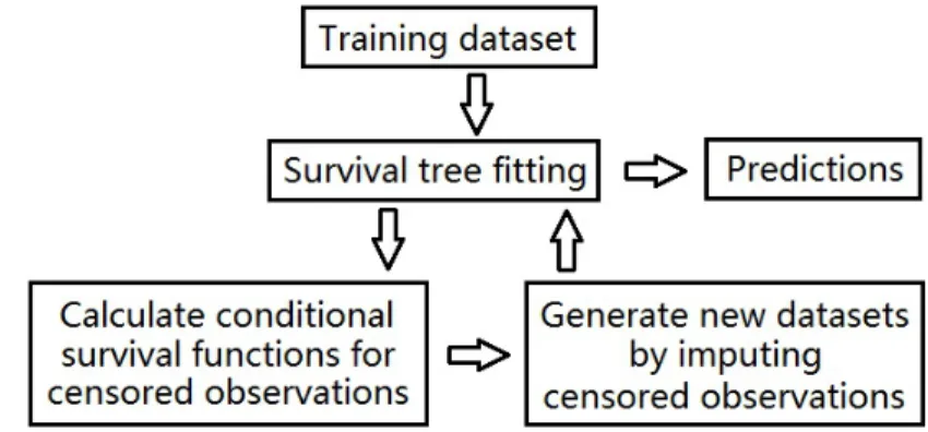
Figure 2.1: A Graphical demonstration of RIST
We will begin our algorithm with a graphical view (Figure ??) followed by a high-level illustration of the framework (Table 2.1), then a detailed description of each step will be given in subsequent sections: Survival tree model fitting (Section 2.3.2), Con-ditional survival distribution (Section 2.3.3), One-step imputation for censored obser-vations (Section 2.3.4), Refit imputed dataset and further calculation (Section 2.3.5), and Final prediction (Section 2.3.6).
2.3.2 Survival tree model fitting
Table 2.1: Algorithm for tree fitting
1. Survival tree model fitting: Generate M extremely randomized survival trees for the raw training data set under the following settings:
a) For each split, K candidate covariates are randomly selected from p covariates, along with random split points. The best split, which provides the most distinct daughter nodes, is chosen.
b) Any terminal node should have no less thannmin>0 observed events.
2. Conditional survival distribution: A conditional survival distribution is calcu-lated for each censored observation.
3. One-step imputation for censored observations: All censored data in the raw training data set will be replaced (with correctly estimated probability) by one of two types of observations: either an observed failure event with Y < τ , or, a censored observation withY =τ.
4. Refit imputed dataset and further calculation: M independent imputed datasets are generated according to 3, and one survival tree is fitted for each of them using 1.a) and 1.b).
5. Final prediction: Step 2–4 are recursively repeated a specified number of times before final predictions are calculated.
(2001)’s Random Forests approach are that, first, the splitting value is chosen fully at random; second, the whole training set is used instead of only bootstrap replicates. M
independent trees are fit to the entire training dataset as follows. For each tree, when reaching a node to split, K covariates along with one random split point per covariate are chosen from all non-constant covariates (splitting will stop if all covariates are constant). In our model fitting, the log-rank test statistic is used to determine the best split among the K covariates which provides the most distinct daughter nodes. Once a split has been selected, each terminal node is split again using the same procedure until no further splitting can be done without causing a terminal node to have fewer than nmin events (i.e. observations with δ= 1). We will treat each terminal node as a
2.3.3 Conditional survival distribution
Calculations of conditional survival functions will be made first on the node level, then averaged over all M trees. For the lth terminal node in the mth tree, since there
are at leastnmin failure events, a Kaplan-Meier estimate of the survival function can be
calculated within the node, which we denote by ˆSl
m(t), where t ∈[0, τ]. Noticing that
for any particular subject, that subject eventually falls into only one terminal node for each fitted tree model, we can drop the index “l”. Hence we denote the single-tree survival function by ˆSi
m for theith subject. Averaging over M trees, we have the forest
level survival function ˆSi = M1
∑M m=1Sˆ
i
m. Now, given a subject i that is censored at
time c, i.e., Yi = c and δi = 0, one can approximate the conditional probability of
survival, P(Ti > t|Ti > c), by
s∗i =
1 if t∈[0, c]
ˆ
Si(t)/Sˆi(c) if t∈(c, τ]
(2.1)
Furthermore, we forces∗i(τ+) = 0 by imposing a point mass at timeτ. This point mass will represent the probability that the conditional failure time is larger thanτ.
2.3.4 One-step imputation for censored observations
When subject i is censored, the true survival time Ti is larger than Ci. However, if
in Section 2.3.3. To do so, we generate a new observation Yi∗ from this distribution function and treat it as the observed value if the subject were followed from time 0. Due to the construction of s∗i, Yi∗ must be between Yi and τ. If Yi∗ < τ, then we assume
that Ti is less than τ, and we replace Yi by this new observation Yi∗ with censoring
indicator δ∗i = 1. If Yi∗ = τ, then we assume that the subject has Ti greater than τ,
and we replace Yi by τ with censoring indicator δ∗i = 0. This updating procedure is
independently applied to all censored observations. This gives us a one-step imputed dataset. Note that the observed failure events in the dataset are not modified by this procedure.
2.3.5 Refit imputed dataset
Using the imputation procedure that we introduced in section 2.3.4, we indepen-dently generate M imputed datasets, and fit a single extremely randomized tree to each of them. We pool the M trees to assess the new model structure and survival function estimations. Subsequently, the new conditional censoring distribution can be calculated for each censored observation in the original dataset conditional on their corresponding original censoring value. The original censored observations can thus be again imputed. A new set of imputed datasets can be then generated to assess the next cycle model structure. Hence, a recursive form is established by repeating the model fitting procedure and imputation procedure. Note the term “original” here refers to the raw dataset before imputation. In other words the “conditional survival function” is always conditional on the original censoring time Yi.
This recursive approach can be repeated multiple times prior to the final step. Each time, the imputation is obtained by applying the current conditional survival function estimate to the original censored observations. We denote the process involving q
imputations as q-fold RIST, or simply RISTq.
2.3.6 Final prediction
The final prediction can be obtained by calculating node level estimation and then averaging over all trees in the final model fitting step. For a given new subject with covariates Xnew = (Xnew
1 , ..., Xpnew), denote Snew(·) to be the true survival function
for this subject. Dropping this subject down the mth tree, it eventually falls into a
terminal node (which we label as node l). Note that all the observations in this node are either observed events beforeτ, or censored atτ, and we will treat all observations in a terminal node as i.i.d. samples from the same distribution. To estimate Snew(t),
we employ an empirical type estimator which can be expressed, in the mth tree, as ˆ
Smnew(t) = ∑
i∈node l
I{Yi>t}
φm(l) where φm(l) denotes the size of node l in the m
th tree. Then
the final prediction can be calculated as follows:
and Sˆnew(t) = 1
M M
∑
m=1
ˆ
Smnew(t). (2.2)
2.4 Simulation Studies
(RF) approach utilizes inverse probability of censoring (IPC) weights (Van der Laan and Robins, 2003) and analyzes right censored survival data using log-transformed survival time. The above two methods are implemented through R-packages “random-SurvivalForest” and ”party”. It also interesting to compare our method to the Cox model with regularization. Although the Cox model has significant advantages over tree-based models when the proportional hazards model is the true data generator, it is still important to see the relative performance of tree-based models under such cir-cumstances. The Cox model fittings are implemented through the R-package “glmnet” (Friedman et al., 2010; Simon et al., 2011).
2.4.1 Simulation settings
To fully demonstrate the performance of RIST, we construct the following five scenarios to cover a variety of aspects that usually arise in survival analysis. The first scenario is an example of the proportional hazards model where the Cox model is expected to perform best. The second and third scenarios represent mild and severe violations of the proportional hazards assumption. The censoring mechanism is another important feature that we want to investigate. In Scenario 4, both survival times and censoring times depend on covariate X, however, they are conditionally independent. Scenario 5 is an example of dependent censoring where censoring time not only depends on X but is also a function of survival time T. Although this is a violation of our assumption, we want to demonstrate the robustness of RIST. Now we describe each of our simulation settings in detail:
Scenario 1: A proportional hazards model adapted from Section 4 of Ishwaran et al. (2008), we let p = 25 and X = (X1, ..., X25) be drawn from a multivariate
normal distribution with covariance matrix V, where Vij = ρ|i−j| and ρ is set to 0.9.
µ=b0×
∑20
i=11xi, whereb0 is set to 0.1. Censoring times are drawn independently from
an exponential distribution with mean set to half of the average of µ. Study length τ
is set to 4. Sample size is 200 and the censoring rate is approximately 30%.
Scenario 2: We draw 10 i.i.d. uniform distributed covariates and use link function
µ= sin(x1×π) + 2× |x2−0.5|+x33 to create a violation of the proportional hazards
assumption. Survival times follow an exponential distribution with meanµ. Censoring times are drawn uniformly from (0, τ) whereτ = 6. Sample size is 200 and the censoring rate is approximately 24%.
Scenario 3: Letp= 25 andX = (X1, ..., X25) be drawn from a multivariate normal distribution with covariance matrix V, whereVij =ρ|i−j| and ρ is set to 0.75. Survival
times are drawn independently from a gamma distribution with shape parameter µ= 0.5 + 0.3×|∑15i=11xi|and scale parameter 2. Censoring times are drawn uniformly from (0,1.5×τ) and the study length τ is set to 10. Sample size is 300 and the censoring rate is approximately 20%.
Scenario 4: We generate a conditionally independent censoring setting where p= 25 and X = (X1, ..., X25) are drawn from a multivariate normal distribution with covariance matrix V, where Vij =ρ|i−j| and ρ is set to 0.75. Survival times are drawn
independently from a log-normal distribution with mean set to µ= 0.1× |∑5i=1xi|+ 0.1× |∑25i=21xi|. Censoring times follow the same distribution with parameterµ+ 0.5. Study length τ is set to 4. Sample size is 300 and the censoring rate is approximately 32%.
Scenario 5: This is a dependent censoring example. We let p = 10 and X = (X1, ..., X10) be drawn from a multivariate normal distribution with covariance matrix
V, whereVij =ρ|i−j|andρis set to 0.2. Survival timesT are drawn independently from
an exponential distribution with meanµ= (1+eex1+x1+x2+x2+x3x3). A subject will be censored at
size is 300 and the censoring rate is approximately 27%.
2.4.2 Tuning parameter settings
All three tree-based methods offer a variety of tuning parameter selections. To make our comparisons fair, we will equalize the common tuning parameters shared by all methods and set the other parameters to the default. According to Geurts et al. (2006); Ishwaran et al. (2008) the number of covariates considered at each splitting,
K, is set to the integer part of√p where pis the number of covariates. For RIST and RSF, the minimal number of observed failures in each terminal node,nmin, is set to 6.
The counterpart of this quantity in the RF, minimal weight for terminal nodes is set to the default. For RSF and RF, 1000 trees were grown. Two different splitting rules are considered for RSF: the log-rank splitting rule and the random log-rank splitting rule (see Section 6 in Ishwaran et al. (2008)). In the RF, a Kaplan-Meier estimate of the censoring distribution is used to assign weights to the observed events. The imputation process in RIST can be done multiple times before reaching a final model. Here we consider 1, 3, and 5 imputation cycles withM = 50 trees in each cycle (namely 1-fold, 3-fold, and 5-fold RIST).
The Cox models are fit with penalty termλPα(β) =λ[(1−α)/2||β||22+α||β||]. We
use the lasso penalty by setting α = 1. The best choice for λ is selected using the default 10-fold cross-validation.
2.4.3 Prediction Error
To be more specific, let S(t) denote the true survival function and let ˆS(t) denote its estimate. Integrated absolute error is defined as∫0τ|S(t)−Sˆ(t)|dt and Supremum ab-solute error is defined as sup
0≤t≤τ|
S(t)−Sˆ(t)|. Noticing that both measurements require knowledge of the true data generator, which is typically not known in practice, we also utilize the widely adopted integrated Brier score (Graf et al., 1999; Hothorn et al., 2006) as a measure of performance since it can be calculated from observed data only. The Brier score for censored data at a given time t >0 is defined as
BS(t) = 1
N N
∑
i=1
{ ( ˆS(t|Xi))2I(Yi ≤t∧δi = 1) ˆG(Yi)−1
+(1−Sˆ(t|Xi))2I(Yi > t) ˆG(Yi)−1 }, (2.3)
where ˆG(·) denotes the Kaplan-Meier estimate of the censoring distribution. The inte-grated Brier score is further given by
IBS =max(Yi)−1
∫ max(Yi)
0
BS(t)dt. (2.4)
In the simulation study validation set, where the failure times are fully observed, ˆG(t) reduces to 1 andδ = 1. The integrated Brier score can then be viewed as a degenerate version of an L2 measure of the survival function estimation error. In our simulations, the Brier score is only calculated up to the maximum study length τ since there is no information available beyondτ in the training dataset. Hence the integrated Brier score in our simulation study is defined byIBS =τ−1∫τ
0 BS(t)dt. Note that this definition
will also prevent errors at larget from dominating the results.
selected subjects. To compare the risks of two subjects, RIST uses area under the predicted survival curve; RSF uses cumulative survival function; the RF uses predicted survival time; and the Cox model uses the link function. A detailed calculation of the C-index algorithm is given in Ishwaran et al. (2008), and the prediction error is defined as 1 minus the C-index.
2.4.4 Simulation results
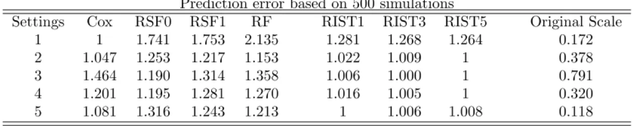
Each simulation setting is replicated 500 times and results are presented in the following tables. For convenience, within each scenario, we use the best method in terms of performance as the reference group which we rescale to 1. Prediction errors for all other methods are scaled and presented as a ratio to the reference group, i.e. prediction errors larger than 1 will indicate a worse performance. The last column is the original scale multiplier. Major findings are summarized below:
1. In all simulation settings with survival function prediction error, RIST performs better than the other two tree-based methods and the improvements are sig-nificant. For example, under the proportional hazards model (Scenario 1) with integrated absolute error of the survival function (Table 2), RSF0 and RF perfor-m 37.7% and 68.9% worse than RIST respectively. In all other scenarios, RIST performs at least 19% better than RSF and the improvements can be up to 31.4% better in terms of this error measurement. For supremum error, RIST performs 21.6∼ 55.5% better than RF and improvements over RSF generally lie between 10 ∼ 20%. Improvements in terms of integrated Brier score are less impressive due to the large variability when generating the survival times, however, perfor-mances of RIST are uniformly better than RSF and RF.
violated, performance of the Cox model can be over 40% worse than RIST in terms of both integrated and supremum survival error. On the other hand, un-der the proportional hazards model, the Cox model performs 26.4% better than RIST. However, when compared to RSF0 and RF (which 74.1% and 113.5% worse than the Cox model), RIST still shows a much stronger performance relative to the other tree-based methods.
3. If we focus on the worst performing scenario for each method, we can see that the robustness of RIST is superior to any competing methods. In fact, RIST is the most robust in terms of all three survival function estimation errors. And RIST never falls into the “worst two” category in any situation using any error measurement, whereas all other methods always, at some point, fail to compete with the others (i.e., has largest prediction error).
4. 3-fold and 5-fold RIST generally perform better than 1-fold RIST, however, higher-fold imputation does not always further improve the performance. The reason is that after several cycles of imputation, the model structure tends to have stabilized. This might also possibly be due to overfitting in certain settings. Scenario 5 represents a dependent censoring case which violates our model as-sumptions, and slight overfitting can be seen. This phenomenon indicates that our imputation procedure is somewhat sensitive to the information carried by censored observations, but not excessively so. Nevertheless, severe violation of the independent censoring assumption could further downgrade the performance of RIST.
clearly superior to any tree-based models, RSF1 still shows an even lower C-index error than the Cox model. Hence interpretability of the C-index is sometimes unclear.
6. Performance of the RF method is generally not as strong as the other approaches. The likely reason is that this method utilizes inverse probability of censoring (IPC) which relies heavily on the assumption that G(T|X) = P(C > T|X) is strictly greater than zero almost everywhere. However, in real life study designs, such as in clinical trials running for a predefined period, this assumption is violated (Hothorn et al., 2006). Under such circumstances, the estimation of mean survival time would be expected to be biased.
Table 2.2: Integrated absolute error for survival function† Prediction error based on 500 simulations
Settings Cox RSF0 RSF1 RF RIST1 RIST3 RIST5 Original Scale
1 1 1.741 1.753 2.135 1.281 1.268 1.264 0.172
2 1.047 1.253 1.217 1.153 1.022 1.009 1 0.378
3 1.464 1.190 1.314 1.358 1.006 1.000 1 0.791
4 1.201 1.195 1.281 1.270 1.016 1.005 1 0.320
5 1.081 1.316 1.243 1.213 1 1.006 1.008 0.118
Table 2.3: Supremum absolute error for survival function ‡ Prediction error based on 500 simulations
Settings Cox RSF0 RSF1 RF RIST1 RIST3 RIST5 Original Scale
1 1 1.364 1.361 1.788 1.151 1.150 1.151 0.073
2 1.075 1.120 1.014 1.216 1.002 1.003 1 0.112
3 1.438 1.113 1.157 1.375 1.001 1 1.001 0.139
4 1.250 1.134 1.103 1.340 1.002 1.000 1 0.142
5 1 1.323 1.238 1.399 1.198 1.204 1.206 0.082
†: Integrated absolute error for survival function is defined as∫τ
0 |S(t)−Sˆ(t)|dt.
‡: Supremum absolute error for survival function is defined as sup
0≤t≤τ
|S(t)−Sˆ(t)|.
RSF0 and RSF1 are Random Survival Forests using logrank and random logrank splitting rules respectively. RIST1, RIST3, and RIST5 are 1-fold, 3-fold, and 5-fold RIST respectively.
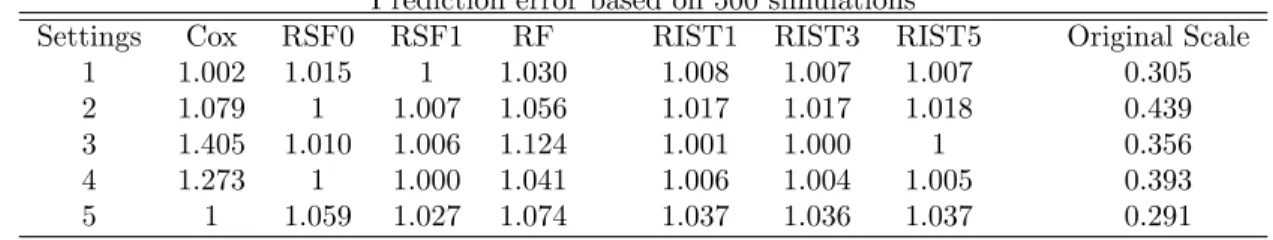
Table 2.4: C-index error Prediction error based on 500 simulations
Settings Cox RSF0 RSF1 RF RIST1 RIST3 RIST5 Original Scale
1 1.002 1.015 1 1.030 1.008 1.007 1.007 0.305
2 1.079 1 1.007 1.056 1.017 1.017 1.018 0.439
3 1.405 1.010 1.006 1.124 1.001 1.000 1 0.356
4 1.273 1 1.000 1.041 1.006 1.004 1.005 0.393
5 1 1.059 1.027 1.074 1.037 1.036 1.037 0.291
Table 2.5: Integrated Brier score Prediction error based on 500 simulations
Settings Cox RSF0 RSF1 RF RIST1 RIST3 RIST5 Original Scale
1 1 1.038 1.037 1.135 1.018 1.017 1.017 0.125
2 1.009 1.008 1.007 1.020 1.000 1.000 1 0.130
3 1.101 1.022 1.041 1.094 1.000 1.000 1 0.128
4 1.044 1.018 1.032 1.063 1.001 1.000 1 0.124
5 1.059 1.021 1.014 1.028 1.000 1 1.001 0.116
RSF0 and RSF1 are Random Survival Forests using logrank and random logrank splitting rules respectively. RIST1, RIST3, and RIST5 are 1-fold, 3-fold, and 5-fold RIST respectively.
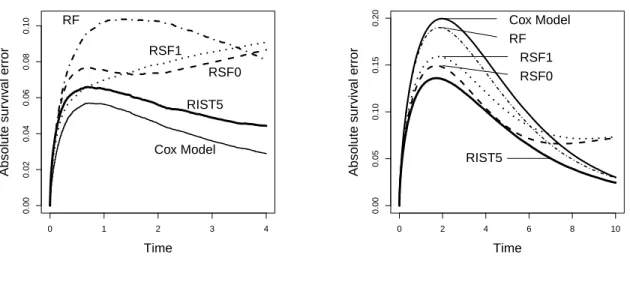
Figure 2.2: Proportional Hazards Model
0 1 2 3 4
0.00 0.02 0.04 0.06 0.08 0.10 Time Absolute sur viv al error RF RSF1 RSF0 RIST5 Cox Model
Figure 2.3: Non-Proportional Hazards
0 2 4 6 8 10
0.00 0.05 0.10 0.15 0.20 Time Absolute sur viv al error Cox Model RF RSF1 RSF0 RIST5
2.5 Data Analysis
In this section we compare RIST with RSF, RF, and the Cox model on two datasets: the German Breast Cancer Study Group (GBSG) data and the Primary Biliary Cir-rhosis (PBC) data. We use Brier score and integrated Brier score as the criteria for comparison. The integrated Brier score, as we observed in the simulation studies, pro-vides a slightly more sensitive measurement than the C-index. A random assignment algorithm (a slight modification from Ishwaran et al. (2008)) is also being introduced to handle missing covariate data in the PBC data section.
2.5.1 Breast Cancer Data
2.5.1.1 Data description
By March 31, 1992, median follow-up time was 56 months with 197 events for disease-free survival and 116 deaths observed. The recurrence-free survival times of the 686 patients (with 299 events) who had complete data were analyzed in Sauerbrei and Royston (1999). The p = 8 observed factors are age, tumor size, tumor grade, number of positive lymph nodes, menopausal status, progesterone receptor, estrogen receptor, and whether or not hormonal therapy was administered. There is no missing data. This data-set has been studied by both Ishwaran et al. (2008) and Hothorn et al. (2006) for tree types of model fitting, hence we also utilize this dataset in our paper.
We randomly divide the dataset into two equal sized subsets, and then use one as a training set and the other as a validation set. 500 independent training datasets were thus generated and prediction error calculated according to the corresponding validation sets. All parameter settings are identical to those given in Section2.4.2.
2.5.1.2 Results
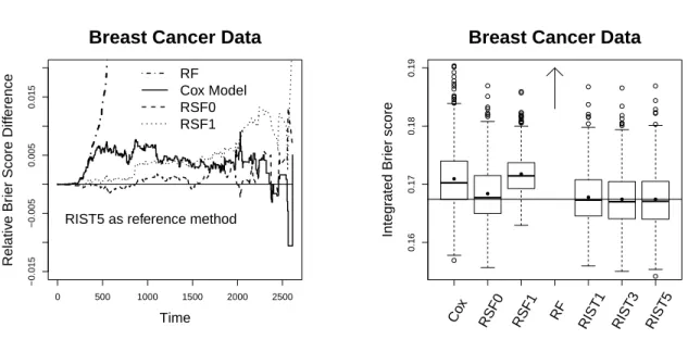
We present the relative over-time Brier scores in Figure 4 (using 5-fold RIST as the reference group, and subtracted from each method accordingly). The plot is constructed so that worse performance compared to 5-fold RIST is above 0. The Brier score for RF is significantly distinct from other methods and its relative Brier score is over 0.15 more than RIST towards the end of study. Among all other methods, RIST and RSF0 performs similar, while RIST has lower Brier score at a majority of time points across the entire range. The Cox model and RSF1 perform worse than the above two; however, they both perform significantly better than RF.
The boxplot for integrated Brier scores are shown in Figure 5. The boxplot for RF is above the upper bound (with mean 0.2535 and 1st, 2nd, and 3rdquartiles 0.2438, 0.2529,
terms of both mean and median integrated Brier score. The improvement compared to the Cox model, RSF1 and RF, is significant. RSF0 performs close to RIST, however RIST5 has lower integrated Brier score than RF0 in 62.2% of the simulations, and out-performs the Cox model and RSF1 in 78.8% and 93.8% of the simulations respectively. A variable importance (Breiman, 2001; Ishwaran, 2007) analysis is done by using the validation set to assess the variable importance measure. However, similar results were found among all tree-based methods.
Figure 2.4: Relative Brier score
0 500 1000 1500 2000 2500
−0.015
−0.005
0.005
0.015
Time
Relativ
e Br
ier Score Diff
erence
RIST5 as reference method RF Cox Model RSF0 RSF1 Breast Cancer Data
Figure 2.5: Integrated Brier score
Integr
ated Br
ier score
0.16
0.17
0.18
0.19
Co x
RSF0 RSF1 RF RIST1 RIST3 RIST5 Breast Cancer Data
2.5.2 PBC Data
2.5.2.1 Data description
This Mayo clinical trial study was conducted between 1974 and 1984 and the study analysis time was in July, 1986. A total of 424 PBC patients, referred to the Mayo clinic during that ten-year interval, met the eligibility criteria for the randomized tri-al. 312 cases in the dataset participated in the randomized trial and contain largely complete data and hence will be used in our analysis. The additional 112 cases did not participate in the clinical trial and these data will not be used. The data contains 17 co-variates including treatment, age, sex, ascites, hepatomegaly, spiders, edema, bilirubin, cholesterol, albumin, urine copper, alkaline phosphatase, SGOT, triglicerides, platelets, prothrombin time, and histologic stage of disease.
As with the breast cancer example, we randomly divide the PBC data set into a training dataset and a validation set with equal sample size and independently repeat this 500 times. Model parameter settings here are also the same as in the breast cancer example.
2.5.2.2 Missing covariate method
Missing data is an issue in the PBC dataset. Among the 312 subjects, there are 28 subjects with missing cholesterol measurements, 30 with missing triglicerides surements, 2 with missing urine copper measurements and 4 with missing platelet mea-surements. There are 276 subjects with complete measurements for all covariates. Our algorithm for handling missing data is very similar to Ishwaran et al. (2008), where the missingX values are randomly generated from the empirical distribution of the in-bag observations in a node. Ishwaran et al. (2008)’s method will be implemented in both RSF0 and RSF1.
is calculated by omitting the subjects that have missing Xp value. When the splitting
variable is chosen and daughter nodes are built, those subjects with missing splitting variable are randomly assigned to either daughter node with probabilities proportional to the sizes of the daughter nodes. This random assignment algorithm is also applied during the prediction process. Suppose we drop a subject with missing covariate Xp
down a single tree. Whenever Xp is required to determine which further node it falls
into, we randomly throw this subject into either node with probability proportional to node size as described above.
2.5.2.3 Results
Similar to the Breast Cancer data analysis, we present the relative over-time Brier scores in Figure 6 using 5-fold RIST as the reference group. The Brier score of RF increases dramatically as time increases. We restrict our plotting frame so that we can focus more on the differences between the other methods. The Brier score of the Cox model and RSF1 is higher than RIST5 at almost every time over the entire study duration. RSF0 has higher prediction error than RIST5 at most time points, however, it out-performs RIST5 towards the end of study.
Figure 2.6: Relative Brier score
0 1000 2000 3000 4000
−0.02 0.00 0.01 0.02 0.03 0.04 0.05 Time Relativ e Br
ier Score Diff
erence
RIST5 as baseline
Cox Model RSF1
RF
RSF0
PBC Data
Figure 2.7: Integrated Brier score
0.11 0.12 0.13 0.14 0.15 0.16 0.17 Integr ated Br ier score Co x
RSF0 RSF1 RF RIST1 RIST3 RIST5
PBC Data
2.6 Discussion
In this paper, we introduced recursively imputed survival trees (RIST), a novel cen-soring imputation approach integrated with a tree-based regression method for right-censored survival data. While preserving information carried by the right-censored observa-tions (by calculating conditional survival distribution), the imputation method extends the utility of censored observations and uses the updated conditional failure information to improve model prediction. The regression procedure is built on the newly developed tree method, extremely randomized trees (Geurts et al., 2006), which is an alternative to Breiman’s popular random forests method. Through a recursive algorithm, both the model fitting processes and the imputation processes affect each other, and the performances of both improve simultaneously.
2.6.1 Why RIST works
further understand this new approach.
One potential advantages of RIST comes from the tree-based modeling point of view. Since the entire training set is used to build each single tree, extremely randomized trees can build larger models (i.e with more terminal nodes) compared to Random Forests which use bootstrap samples. Furthermore, after the first imputation cycle, additional observed events are created which allow each tree to grow even deeper. One may wonder whether this could cause over-fitting; however, the random generation of the imputed values provides sufficient diversity which will help eliminate over-fitting.
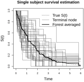
Moreover, we found that the Monte Carlo EM (MCEM) algorithm (Wei and Tanner, 1990; McLachlan and Krishnan, 2007) is the best way to explain our proposed procedure theoretically. The random generation of imputed values can be viewed as the Monte Carlo E-step without taking the average of all randomly generated sample points, while the survival tree fitting procedure is explicitly an M-step to maximize the nonparametric model structure. The “random E-step” imputation procedure does not only preserve the information carried by censored observations, but it also introduces an extra level of diversity into the next-level of model fitting. As is well known, diversity is one of the driving forces behind the success of ensemble methods as has been addressed by many researchers, including Breiman (2001); Dietterich (2000). An interesting phenomenon of diversity can be seen when averaging the terminal node survival function estimation over the forest. Figure 8 (of a subject from Scenario 2) shows that even though an individual terminal node estimation (using nmin observed events) could have a high
conditional survival function estimations can therefore be even further improved.
Figure 2.8: Diversity and forest averaging
0 1 2 3 4 5 6
0.0
0.2
0.4
0.6
0.8
1.0
Time
S(t)
True S(t) Terminal node Forest averaged Single subject survival estimation
The effect that we have seen over the imputation cycle can also be visually explained as a “blurring effect” in optics: While each model fitting step sums up all information from adjacent observations of the target point in the feature space, similar effects also happen to other adjacent observations simultaneously. The next imputation step allows information from remote observations to be carried into adjacent censored observations which can be used in calculating the target survival function estimation. Hence, over several imputation cycles, the overall information that defines the target prediction does not come solely from the partitioned neighborhood of the target point, it comes instead from a “blurred” neighborhood that reaches out to a much wilder range.
initial model is not detecting the true signal correctly, such as in a high-dimensional setting or when the model structure is too complicated. My third topic, reinforcement learning trees for survival data, is proposed to solve this problem.
2.6.2 Other Issues
In multi-fold RIST, most of the improvement is gained during the first several imputation cycles. Additional recursive steps of RIST can help adjust the imputed value and the fitted model structure; however, the increments of improvement tend to be small since the model structure stabilizes fairly quickly. Unfortunately, we do not yet have explicit convergence criteria for RIST. However, based on our simulation experience, it appears that 3-fold to 5-fold RIST generally performs best. Although higher fold imputations perform reasonably well and may even be optimal in some settings, over-fitting also appears to be a possibility. In addition, as fold level increasing, the computational intensity also increases. Hence, we do not recommend going beyond 5-fold RIST.
Another issue that has been addressed frequently in tree-based model fitting is the choice of splitting statistics. During our research, we examined the performance of several alternatives to the log-rank statistic, including the supremum log-rank (Kosorok and Lin, 1999) statistics. However, no significant differences in performance of RIST were detected under the simulation settings that we presented.
Chapter 3
Reinforcement learning trees
3.1 Introduction
number p0, where p0 is an educated guess of the number of strong variables which is
usually much smaller than the total number of variables pbut at least as large as the true number of strong variablesp1. Hence whenp0 is properly chosen, the error bounds
can be significantly improved.
We introduce a new philosophy—reinforcement learning—into the tree-based model framework. For a comprehensive review of reinforcement learning within the artificial intelligence field in computer science and statistical learning, we refer to Sutton and Barto (1998). An important characteristic of reinforcement learning is the “peek-at-the-future” notion which benefits the long-term performance rather than short-term performance. The main features we will employ in the proposed method are: first, to choose variable(s) for each split which will bring the largest return from future branching splits rather than only focusing on the immediate consequences of the split. Such a splitting mechanism can break any hidden structure and avoid inconsistency by forcing splits on strong variables even if they do not show any marginal effect; second, progressively muting noise variables as we go deeper down a tree so that even as the sample size decreases rapidly towards a terminal node, the strong variable(s) can still be properly identified from the reduced space. One consequence of the new approach, which we call reinforcement learning trees (RLT), as we will show later, is that the convergence rate should not depend on p, but instead, it depends on a pre-specified valuep0 which is much smaller than p and larger than p1. Hence, whenp0 is properly
chosen, the convergence rate can be greatly improved.
simulation studies and data analyses presented later, we will examine the performance of the newly proposed RLT with both one-dimensional and high-dimensional cuts and show that the benefit can be profound in some situations.
The part of the dissertation is organized as follows. In Section 3.2, we introduce the underlying model and notation to facilitate the formulation of our method. In Section 3.3, we give details of the methodology for the proposed approach. Theoretical results and their interpretation are given in Section 3.4. Most of the details of the proofs will be deferred to the last section. In Sections 3.5 we compare RLT with popular statistical learning tools, such as random forests (Breiman, 2001), BART (Chipman et al., 2010), gradient boosting (Friedman, 2001) and GLM with LASSO (Friedman et al., 2010), using simulation studies and real datasets. Section 3.6 contains some discussion and gives rationale for both the method and asymptotic behaviors. Future research directions are also discussed. The paper concludes with the proofs.
3.2 Statistical model
We consider a regression or classification problem from which we observe a sam-ple of i.i.d. training observations Dn = {(X1, Y1),(X2, Y2), ...,(Xn, Yn)}, where each Xi = (X
(1) i , ..., X
(p)
i )T denotes a set of p variables from a feature space X. For the
regression problem, Y is a real valued outcome with E(Y2)< ∞; and for the
classifi-cation problem, Y is binary outcome that takes values of 0 or 1. We also assume that the expected value E(Y|X) is completely determined by a set of p1 < p variables. We
refer to these p1 variable as “strong variables”, and refer to the remaining p2 =p−p1
variables as “noise variables”. Without loss of generality, we assume that the strong variables are the first p1 variables, which means E(Y|X) = E(Y|X(1), X(2), ..., X(p1)).
the set{1,2, ..., p}.
3.3 Reinforcement learning trees
In short, the proposed reinforcement learning trees are traditional random forests with a special type of splitting variable selection and noise variable muting at each internal node. These features are made available by implementing a reinforcement learning mechanism. Let us first consider an example which demonstrates the impact of reinforcement learning: Assume thatE(Y|X) = I(X(1) >0.5)I(X(2) >0.5), so that
p1 = 2 and p2 = p−2. The difficulty in estimating this structure with conventional
random forests is that neither of the two strong variables show marginal effects. The immediate reward, i.e. reduction in prediction errors, from splitting on these two variables is identical to the reward obtained by splitting on one of the noise variables. Hence, it unlikely that, whenpis relatively large, eitherX(1) orX(2)would be chosen as
the splitting variable. However, if we know in advance that splitting on either X(1) or
X(2) would yield significant rewards down the road for later splits, we could confidently force a split on either variable regardless of the immediate rewards.
How we identify the most important variable at any internal node is to first fit at that node an embedded random forest and acquire the associated variable importance measures for all the covariates. Then we proceed to split the node using the most important variable(s). When doing this recursively for each daughter node, we can focus the splits on the variables which will be very likely to lead to a tree yielding the smallest prediction error in the long run.
have a good idea about which variables are strong and which are not. Therefore, we will utilize this information to progressively mute noise variables during the tree construction process and to gradually restrict the search for splitting variables within a subspace of the entire feature space as the internal node sample sizes get smaller.
The remainder of this section is structured as follows: We first give a higher level algorithm outlining the main features of the RLT method in Section 3.3.1 without specifying the definitions of the subcomponents: embedded model, variable importance, variable deletion, and high-dimensional split. Detailed definitions of these components are given in subsequent subsections. In Sections 3.3.2 and 3.3.3 we give details of how to fit the embedded model and calculate variable importance at each internal node. In Section 3.3.4, we introduce a variable screening method that progressively mutes noise variables at each internal node. In Section 3.3.5, we extend one dimensional splits to high-dimensional splits by utilizing the available variable importance information at each internal node.
3.3.1 Reinforcement learning trees
Table 3.1: Algorithm for reinforcement learning trees
1. DrawM bootstrap samples fromD.
2. For them-th bootstrap sample, wherem∈ {1, ..., M}, fit one RLT modelfbm, using
the following rules:
a) At an internal node A, fit an embedded model fbA∗ to the data in A, restricted to the set of variables{1,2, ..., p}\Pd
A, i.e. P\PAd, where wherePAd is the set of muted
variables at the current nodeA. Details are given in Section 3.3.2.
b) UsingfbA∗, calculate the variable importance measureV IcA(j) for each variableX(j),
wherej∈ P. Details are given in Section 3.3.3.
c) Split nodeA into two daughter nodes using either i) or ii).
i) For a one-dimensional split, use the variable with the largest variable importance measure, namely arg maxjV IcA(j), as the splitting variable. The cut point c is
chosen randomly and uniformly. We call this method RLT1.
ii) For a high-dimensional split, a linear combination of variables is used. Details are given in Section 3.3.5. We call this method RLTk, wherekis the number of variables used in the linear combination.
d) Update the set of muted variable setPd for the two daughter nodes by adding the
variables with the lowest variable importance measures at the current node. Details are given in Section 3.3.4.
e) Apply a)–d) on each daughter nodes until node sample size is smaller than a pre-specified valuenmin.
3. AverageM trees to get a final model fb=M−1∑M
m=1fbm. For classification,fb= I
(
0.5< M−1∑M
m=1fbm )
3.3.2 Embedded model
To assess the variable importanceV IcA(j) for each variablej at any internal nodeA,
we must first fit an embedded model to the internal node data. Note that at the root node, where the set of muted variablesPm =∅, all variables in the setP ={1,2, ..., p}
are considered in the embedded model and their variable importance measures will be assessed. However, as we move further down the tree, some variables will be muted and Pm ̸= ∅, then the embedded model will be fit using only the non-muted variable set P\Pd
A. For the choice of the embedded model, we use random forests (Breiman,
2001). It is not necessary that random forests be used here. Alternatively, any learning method which is verified to be consistent with a certain convergence rate, for example, purely random forests, can be used to estimate the embedded model.
Suppose we are at an internal node A in the tree building process. To be specific, when a one-dimensional split is used, any internal nodeAcan be expressed as a hyper-cube in the feature space, i.e. A={(X(1), ..., X(p)) :X(j)∈(aj, bj]⊆[0,1], forj ∈ P}. Denote the samples at this internal node asDA={(Xi, Yi) :Xi ∈A}. We fit a random
forests model, denoted by fbA∗, to the internal node data DA with only variables that
are in the set P \ Pd
A. For convenience, we use all the default settings in Breiman
(2001) for the embedded random forests. To facilitate our later arguments, we denote the number of trees in the embedded model as M∗ and denote each tree as fbA,m∗ , for
m∈(1,2, ..., M∗).
3.3.3 Variable importance