ISSN: 2302-9285, DOI: 10.11591/eei.v10i1.2007 299
Discretization methods for Bayesian networks in the case
of the earthquake
Devni Prima Sari1, Dedi Rosadi2, Adhitya Ronnie Effendie3, Danardono4
1
Department of Mathematics, Universitas Negeri Padang, Indonesia
2,3,4
Department of Mathematics, Universitas Gadjah Mada, Indonesia
Article Info ABSTRACT
Article history: Received Aug 31, 2019 Revised Dec 10, 2019 Accepted May 5, 2020
The Bayesian networks are a graphical probability model that represents interactions between variables. This model has been widely applied in various fields, including in the case of disaster. In applying field data, we often find a mixture of variable types, which is a combination of continuous variables and discrete variables. For data processing using hybrid and continuous Bayesian networks, all continuous variables must be normally distributed. If normal conditions unsatisfied, we offer a solution, is to discretize continuous variables. Next, we can continue the process with the discrete Bayesian networks. The discretization of a variable can be done in various ways, including equal-width, equal-frequency, and K-means. The combination of BN and k-means is a new contribution in this study called the k-means Bayesian networks (KMBN) model. In this study, we compared the three methods of discretization used a confusion matrix. Based on the earthquake damage data, the K-means clustering method produced the highest level of accuracy. This result indicates that K-means is the best method for discretizing the data that we use in this study.
Keywords: Bayesian networks Earthquake Equal-frequency Equal-width K-means
This is an open access article under the CC BY-SA license.
Corresponding Author: Devni Prima Sari,
Department of Mathematics, Universitas Negeri Padang,
Prof Dr H mk Air Tawar Barat, Padang, Indonesia. Email: [email protected]
1. INTRODUCTION
The Bayesian networks (BN) show a causal probabilistic relationship between a set of random variables, conditional dependency, and a depiction of the joint probability distribution. The two main parts of the Bayesian network are directed acyclic graph (DAG) and a set of conditional probability distributions (CPD). In directed acyclic graphs, nodes represent random variables and causal probabilistic dependency relationships between random variables in the graph are represented by directed arcs [1]. BN can accommodate various sources of knowledge and data types, such as prior experience and expert information [2]. These advantages make the Bayesian networks widely applied in various fields, both in the medical [3, 4], education [5], and economics [6]. BN has also been applied to several disaster cases, such as an earthquake [7-12], flood [13-15], hurricanes [16], and tsunamis [17, 18].
Based on the types of variables, there are three types of BN model; discrete Bayesian networks (DBN) [19], continuous Bayesian networks (CBN) [20], and hybrid Bayesian networks (HBN) [21, 22]. Discrete and continuous Bayesian networks are respectively applied to discrete and continuous variables, whereas hybrid Bayesian networks are applied in cases consisting of a mixture of the two variables. In its application, data is often found with a combination of two variables. If the process is continued with hybrid
Bayesian networks, we will be faced with a problem if the data from continuous variables are not normally distributed.
To simplify the process of research, we offer a solution, which is to assume all discrete variables. Therefore, we carry out a method of discretization for all continuous variables and continue the process using discrete Bayesian networks. Discretization methods commonly used include equal-width [23] and equal frequency [24, 25]. Both of these discretization methods are often found in applied research related to Bayesian networks. However, both of these methods have weaknesses, where equal width is less suitable to be applied to data containing outliers, and equal frequency will be confused if used in experiments containing multiple data with the same values. Therefore, in this study, the authors discretizes using k-means method. Discretization with k-means results in a higher level of model accuracy than that of the two previous discretization methods where the level of accuracy for each of these methods are obtained from a confusion matrix. The combination of BN and k-means is a new contribution in this study called the k-means Bayesian networks (KMBN) model. In this study, we implement discrete Bayesian networks in the case of an earthquake disaster. In particular, we determine the risk of damage to buildings due to an earthquake by considering several factors including, construction, risk of landslides, peak ground acceleration (PGA), distance to faults, slope, earthquake center distance, etc.
2. RESEARCH METHOD
Discretization is a process of changing a continuous variable into a discrete variable. This process is often carried out in data analysis to group several continuous attribute values and to divide these values into intervals so that they do not overlap [26]. We can do variable discretization with two approaches, which are supervised learning and unsupervised learning. Supervised learning is an approach where data is trained, and variables are targeted so that the proposed approach is to group data based on existing data. Meanwhile, if we do not have trained data so that the available data can be grouped into two, three, and so on, then this approach is called unsupervised learning. In this study, we use the method of discretizing unattended learning. This method divides the object into several intervals, where intervals represent the results of variable discretization. The unsupervised discretization process consists of two steps, which decide how many categories to use and map the continuous attribute value to the category value. The following are given three unsupervised discretization methods that can be combined with Bayesian networks, namely equal-width, equal-frequency, and K-means.
2.1. Equal-width
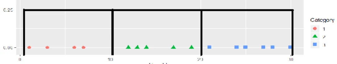
Equal-width is simple discretization methods that divide the range of values observed in each variable, with being the value specified by the user. This process involves sorting the values of continuous variables that are observed by determining the minimum ( ) and maximum ( ) values. The interval can be calculated by dividing the observed value in the same size range using the following equation,
(1)
with a threshold on , . The equal-width method can be applied to discretizing continuous variables [27]. However, this discretization method is sensitive to outliers. The limitation of this method occurs if the distribution of data is uneven, which results in some intervals having more data points than others. A description of the results of discretization with the equal-width method can be identified from Figure 1.
Figure 1. Illustration equal-width method
2.2. Equal-frequency
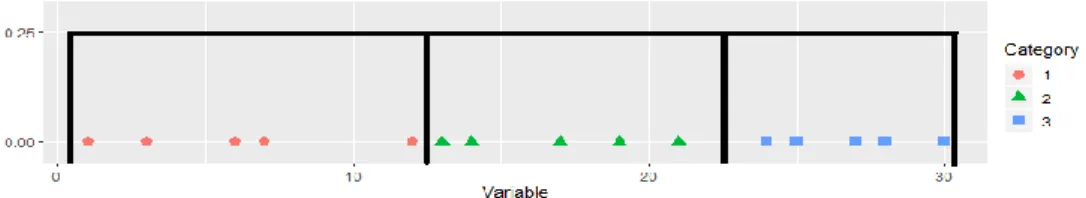
The equal-frequency method determines that the amount of data in each interval is the same. The first step is to sort the value to be discretized from minimum to maximum. Then, divide continuous values sorted
into interval . Each interval contains data with adjacent values, where is the amount of data. Figure 2 shows an illustration of this method in detail. The disadvantage of the equal-frequency method is that it allows the equal value is placed at different intervals.
Figure 2. Illustration equal-frequency method
2.3. K-means discretization
K-means algorithm can be used as a tool to discretize continuous variables. There are only two features in the discretization process. The first feature is a variable to be discretized, and the second feature is an assisted feature that is assumed to be constant. In multivariate statistics, features represent variables. Suppose there is a set of objects * + consisting of objects, and the feature set is
* +, where * + and are constant. Then, the object * +
consists of two features, where is the mth object and the 1st feature and is the mth object and the 2nd feature. The K-means algorithm partitioned objects into clusters. Let * + be the set of clusters so that for and . Next, * + is the set of cluster center (centroid). Cluster has a center where * +.
A measure of the closeness of an object to the centroid , defined as the distance ( ). If the smaller the value of ( ), then more likely that enters the cluster . The distance between the object and centroid can be formulated as follows [28],
( ) (∑ | | ) ⁄ (2)
In this study, we use Euclidean distances as a formula to calculate the closest distance. In the k-means discretization, the process of minimizing the amount of distance between all objects and centroids is carried out using the following equation,
( ) ∑ ∑ ( ) (3)
with constraints
∑ (4)
where * + is an element that represents the membership of th objectand the th cluster.
If , then is placed in the cluster . But if , then is not placed for the cluster . The optimization problem in K-means consists of two sub-problems. There is the process of placing objects into a cluster based on the closest distance between the object and the centroid, and the process of updating all centroid in each cluster [29]. The process of placing objects can be stated in the following equation,
{ ( ) ( ) (5)
Next, the update process of the centroid is expressed as (6). ∑ ∑
(6)
K-means method repeats the placement and update process until all elements of the are the same as the previous value. The following are the steps for the K-means algorithm [30].
a. Determine the number of clusters. b. Determine centroid randomly.
c. Determine the distance of each object to the centroid. The closest distance between an object and a certain centroid determines the placement of objects in the cluster.
d. Calculate the centroid of a new cluster by using the average value of all objects in the cluster. e. Recalculate the distance between each object and the centroid.
f. If the members of the cluster do not change, then the clustering process is complete. Conversely, if it changes, then we back to step 4 until the members of the cluster do not change.
After discretizing all the continuous variables, the next step is to create and analyze the structure using Bayesian networks.
2.4. Bayesian networks
According to Scutari and Denis [20], based on the variable types, there are three types of Bayesian networks that are discrete Bayesian networks, continue Bayesian networks and hybrid Bayesian networks. Discrete Bayesian networks are a BN model in which all the variables involved are discrete and continue Bayesian networks are a BN model constructed by continuous variables. Whereas in Bayesian hybrid networks, there is a combination of discrete and continuous variables. Formal definitions of the Bayesian networks are given in Definition 1. It is consists of a graphical model (i.e., an acyclic directed graph) and a probability for each variable.
Definition 1 [31] Bayesian networks are a pair ( ), where ( ) is an acyclic graph directed with a set of vertices * + for several , and is the set of arcs, and is the probability distribution, indexed by the set of parameters , over n discrete random variables, * +
We can see more clearly about BN in Figure 3. The direction of the arc from node to node shows that random variable affects random variable . While variables and affect variable . In this case, and are called parents, whereas is called a child. The directed arcs representing causal probabilistic dependencies, so cycles are not allowed in the graph. Then, each node in the graph represents the conditional probability distribution [32, 33].
Figure 3. Example of Bayesian networks
For example, assume a simple case like in Figure 3, where we deal with four variables, each of which has three possible states. To represent a joint distribution for variables, we need a table with probability values. The size of the table will increase along with the increasing number of variables until it requires a probability value of for five variables. Inference problems can be derived from the factorization of the distribution of each node obtained from the BN structure, which allows the algorithm to be more efficient for the case. For example, look at the networks in Figure 1, and we are interested in determining the probability of the variable D. Starting from joint distribution, we find that:
( ) ( ) ( | ) ( | )
Then, ( ) it can be written as:
( ) ∑ ( ) ( | ) ( | )
The simple model of Bayesian networks is Naive Bayes, where Naive Bayes assumes the relationship between predictor variables is independent [34, 35].
2.5. K-means Bayesian networks
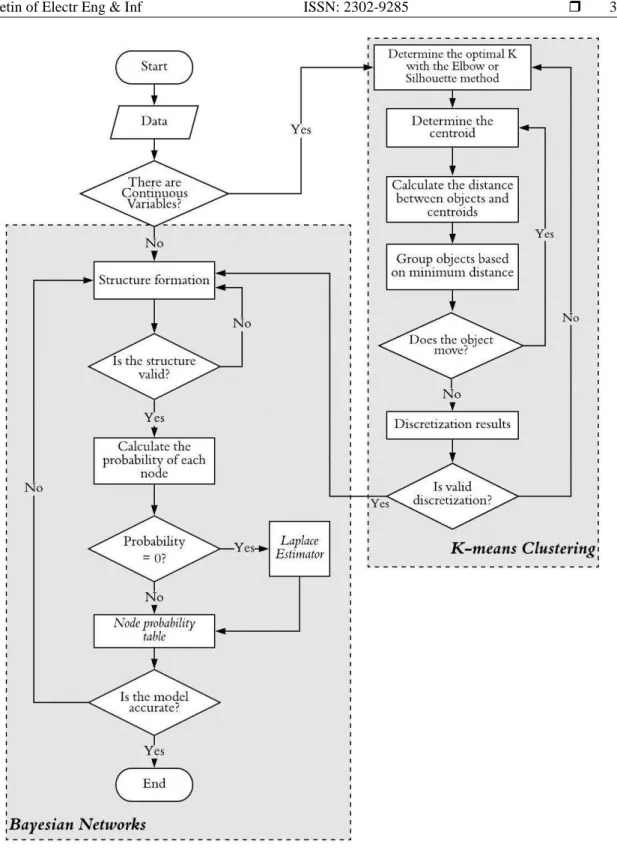
In this study, the K-means algorithm is used for discretizing continuous variables and the Bayesian networks model for classification. The combination of the two is called the KMBN, which is a novelty in this study. For more details, can be seen in Figure 4.
Figure 4. Flowchart of KMBN
3. RESULTS AND DISCUSSION 3.1. Discretization of continuous variables
In this study, 20,702 data of houses were damaged as a result of the 2009 West Sumatra earthquake. The focus of the research was Padang City, which is the capital of West Sumatra Province. The eight variables involved in this study are construction type ( ), peak ground acceleration ( ), epicenter distance ( ), soil type ( ), risk of landslides ( ), slope ( ), distance to fault ( ), and damage rate ( ). From the eight variables, there are three continuous variables; peak ground acceleration ( ), epicenter distance ( ), and distance to fault ( ). Considering the assumption that all variables to be processed must be of a discrete type, all continuous variables will be discretized, where each variable is grouped into three groups.
Basically, different discretization methods will produce different data intervals. Next, we process to the next stage, Bayesian networks, using the output of three discretization methods in Figure 5.
Figure 5. Discretization of epicenter distance ( ), peak ground acceleration ( ), and distance to fault ( )
3.2. Determination of the risk of damage to buildings using BN
The basis for the construction of the BN structure in this study as shown in Figure 6 is based on expert information, with reference to several scientific papers, including Bayraktarli et al. [7, 10], and Li et al. [9, 11]. In this research, we use five exogenous variables and three endogenous variables. Variables that are not affected by other variables are called exogenous variables, while variables that are affected by other variables are called endogenous variables. Construction type ( ), epicenter distance ( ), soil type ( ), slope ( ), and distance to fault ( ) are exogenous variables. Whereas, peak ground acceleration ( ), risk of landslides ( ), and damage level ( ) are endogenous variables. Base on the structure of BN in Figure 6, the global distribution can be factored as follows,
( )
( ) ( ) ( ) ( ) ( ) ( | ) ( | )
( | )
(7)
Next, marginalization is done to get ( ), then ( ) is
( ) ∑ ( ) ( ) ( ) ( ) ( ) ( | )
( | ) ( | )
(8)
with ( ) ( ) ( )
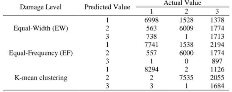
To assess the achievement of the BN model is done using a confusion matrix. The confusion matrix of the damage level based on three different methods can be seen in Table 1. Each column element of a matrix represents the actual value, and the row element represents the predicted value, with the status of the level of damage are slight (1), moderate (2), and heavy (3).
Figure 6. Bayesian networks to determine the level of damage
Table 1. The confusion matrix of damage level in BN discretized uses three different methods
Damage Level Predicted Value Actual Value
1 2 3 Equal-Width (EW) 1 6998 1528 1378 2 563 6009 1774 3 738 1 1713 Equal-Frequency (EF) 1 7741 1538 2194 2 557 6000 1774 3 1 0 897 K-mean clustering 1 8294 2 1126 2 2 7535 2055 3 3 1 1684
Next, the level of accuracy is determined by a proportion between the number of data classified correctly and a total number of test data. The level of accuracy for each BN model is determined using three different discretization methods; equal-width (EW), equal-frequency (EF), and K-means discretization. The results can be seen in Table 2.
Table 2. The level of accuracy is based on three different discretization methods Discretization methods Level of accuracy
Equal-width (EW) 0.71
Equal-frequency (EF) 0.71
K-means discretization 0.85
From Table 2, it can be seen that the highest accuracy of the BN model is obtained using the K-means discretization method with an accuracy rate of up to 85%. Then, it is followed by the equal-width and equal-frequency methods with an accuracy rate of 71%. The low level of accuracy of the model using equal-width because of the limitations of this method in data distribution terms. If the data distribution is not evenly distributed, where some intervals have more data points than others, then this causes the level of accuracy is not optimal if applied in the BN model. Meanwhile, the disadvantage of the equal-frequency method is that there are the same values placed at different intervals.
4. CONCLUSION
BN is an essential tool in measuring uncertainty, especially in terms of determining natural disaster risk. In applications, combinations of variables are often encountered, so the discretization process needs to be carried out for continuous variables. After that, the classification process can be continued with discrete BN. In the case of house damage due to this earthquake, the author uses three distinct discretization methods, that are equal-width, equal-frequency, and K-means. The highest level of accuracy is obtained by using K-means to discrete three continuous variables: peak ground acceleration ( ), epicenter distance ( ), and distance to fault ( ) that is 85%. This research can be developed by focusing on expanding BN software that can contain continuous variables in a flexible and effective form. In further research, the K-Medoids algorithm can be tried as an alternative method to discretizing continuous variables included in the Bayesian network model to reduce sensitivity to outliers.
REFERENCES
[1] M Fiore nd M D C mpos “The Algebr of Directed Acyclic Gr phs ” in Computation, Logic, Games, and Quantum Foundations, Berlin, Springer, pp. 37-51, 2013.
[2] F Noj v n S S Qi n nd C A Stow “Comp r tive An lysis of Discretiz tion Methods in B yesi n networks ”
Environmental Modelling & Software, vol. 87, pp. 64-71, 2017.
[3] M. J. Flores, A. E. Nicholson, A. Brunskill K B Korb nd S M sc ro “Incorpor ting Expert Knowledge When Le rning B yesi n Networks Structure: A Medic l C se Study ” Artificial Intelligence In Medicine, vol. 53, no. 3 pp. 181-204, 2011.
[4] P. Fuster-Parra, P. Tauler, M. Bennasar-Veny, A. Ligeza, A. A. López-González nd A Aguiló “B yesi n Networks Modeling: A C se Study of n Epidemiologic System An lysis of C rdiov scul r Risk ” Computer Methods and Programs in Biomedicine, vol. 126, pp. 128–142, 2016.
[5] J. Laru, P. Näykki, and S Järvelä “Supporting Sm ll-Group Learning Using Multiple Web 2.0 Tools: A Case Study in the Higher Educ tion Context ” The Internet and Higher Education, vol. 15, no. 1, pp. 29-38, 2012. [6] S Hosseini nd K B rker “A B yesi n Networks Model for Resilience-B sed Supplier Selection ” International
Journal of Production Economics, vol. 180, pp. 68-87, October 2016.
[7] Y Y B yr kt rli J P Ulfkj er U Y zg n nd M H F ber “On the Applic tion of B yesi n Prob bilistic Networks for Earthqu ke Risk M n gement ” in Proceedings of the Ninth International Conference on Structural Safety and Reliability, Rome, pp. 20-23, 2005.
[8] Y Y B yr kt rli U Y Aless R D zio nd M H F ber “C p bilities of the B yesi n Prob bilistic Networks Appro ch for E rthqu ke Risk M n gement ” in First European Conference on Earthquake Engineering and Seismology, Geneva, 2006.
[9] L F Li J F W ng nd H Leung “Using Sp ti l An lysis nd B yesi n Networks to Model the Vulner bility nd Make Insurance Pricing of C t strophic Risk ” International Journal of Geographical Information Science, vol. 24, no. 12, pp. 1759-1784, 2010.
[10] Y Y B yr kt rli J W B ker nd M H F ber “Uncert inty Tre tment in E rthqu ke Modeling Using B yesi n Probabilistic Networks ” Georisk, vol. 5, no. 1, pp. 44-58, 2011.
[11] L F Li J W ng H Leung nd S Zh o “A B yesi n Method to Mine Sp ti l D t Sets to Ev lu te the Vulner bility of Hum n Beings to C t strophic Risk ” Risk Analysis: An International Journal, vol. 32, no. 6, pp. 1072-1092, 2012.
[12] D P S ri D Ros di A R Effendie nd D n rdono “Dis ster Mitig tion Solutions with B yesi n Network ” AIP Conference Proceedings, vol. 2192, no. 1, 2019.
[13] Shao-Zhong Zhang, Nan-Hai Yang and Xiu-Kun Wang, "Construction and application of Bayesian networks in flood decision supporting system," Proceedings. International Conference on Machine Learning and Cybernetics, Beijing, Chinapp, vol. 2, 718-722, 2002.
[14] J. Y. Shin, M. Ajmal, J. Yoo, and T W Kim “A B yesi n Networks-Based Probabilistic Framework for Drought Forec sting nd Outlook ” Advances in Meteorology, vol. 2016, pp. 1-10, 2016.
[15] A. D'Addabbo, A. Refice, G. Pasquariello, F. P. Lovergine, D. Capolongo and S. Manfreda, "A Bayesian Network for Flood Detection Combining SAR Imagery and Ancillary Data," in IEEE Transactions on Geoscience and Remote Sensing, vol. 54, no. 6, pp. 3612-3625, June 2016.
[16] L Li J W ng nd C W ng “Typhoon Insur nce Pricing with Sp ti l Decision Support Tools ” International Journal of Geographical Information Science, vol. 19, no. 3, pp. 363-384, 2005.
[17] L Bl ser M Ohrnberger C Riggelsen nd F Scherb um “B yesi n Belief Networks for Tsun mi W rning Decision Support ” in European Conference on Symbolic and Quantitative Approaches to Reasoning and Uncertainty, Springer, Berlin, Heidelberg, 2009.
[18] L Bl ser M Ohrnberger C Riggelsen A B beyko nd F Scherb um “B yesi n Networks for Tsun mi E rly W rning ” Geophysical Journal International, vol. 185, no. 3, pp. 1431–1443, 2011.
[19] C Bielz nd P L rr ñ g “Discrete B yesi n Networks Cl ssifiers: A Survey ” Journal ACM Computing Surveys, vol. 47, no. 1, pp. 1-43, 2014.
[20] M Scut ri nd J B Denis “B yesi n Networks with ex mples in R ” London: Ch pm n nd H ll 2015
[21] P P Shenoy nd J C West “Inference in Hybrid B yesi n Networks Using Mixtures of Polynomi ls ”
International Journal of Approximate Reasoning, vol. 52, no. 5, pp. 641-657, July 2011.
[22] A S lmerón R Rumí H L ngseth T D Nielsen nd A L M dsen “A Review of Inference Algorithms for Hybrid B yesi n Networks ” Journal of Artificial Intelligence Research, vol. 62, pp. 799-828, 2018.
[23] Y W ng Z W ng S He nd Z W ng “A Pr ctic l Chiller F ult Di gnosis Method B sed on Discrete B yesi n Networks ” International Journal of Refrigeration, vol. 102, pp. 159-167, June 2019.
[24] M. D. Lima, S. M. Nassar, P. I. R. Rodrigues, P. J. F. Filho nd C M J cinto “Heuristic Discretiz tion Method for B yesi n Networks ” Journal of Computer Science, vol. 10, no. 5, pp. 869-878, 2014.
[25] R Ropero S Renooij nd L C v n der G g “Discretizing Environment l D t for Le rning B yesi n-Networks Cl ssifiers ” Ecological Modelling, vol. 368, pp. 391-403, January 2018.
[26] A Gupt K G Mehrotr nd C Moh n “A Clustering-B sed Discretiz tion for Supervised Le rning ” Statistics & Probability Letters, vol. 80, no. 9–10, pp. 816-824, 1–15 May 2010.
[27] J Dougherty R Koh vi nd M S h mi “Supervised nd Unsupervised Discretiz tion of Continuous Fe tures ” in
Proceedings of the Twelfth International Conference on Machine Learning, Tahoe City, California, pp. 194-202, 9–12 July 1995.
[28] L Himmelsp ch D Hommers nd S Conr d “Cluster Tendency Assessment for Fuzzy Clustering of Incomplete D t ” in Proceedings of the 7th conference of the European Society for Fuzzy Logic and Technology, Aix-les-Bains, pp. 290-297, 2011.
[29] J T Chi E C Chi nd R G B r niuk “k-POD: A Method for K-Me ns Clustering of Missing D t ”
The American Statistician, vol. 70, no. 1, pp. 91-99, 2016.
[30] A Agr w l nd H Gupt “Glob l K-Me ns (GKM) Clustering Algorithm: A Survey ” International Journal of Computer Applications, vol. 79, no. 2, pp. 20-24, 2013.
[31] T. Koski and J. Noble, “Bayesian networks: An Introduction ” United Kingdom: John Wiley & Sons, Ltd., 2009. [32] D. P. Sari, D. Rosadi, A. R. Effendie and Danardono, "Application of Bayesian network model in determining
the risk of building damage caused by earthquakes," 2018 International Conference on Information and Communications Technology (ICOIACT), Yogyakarta, pp. 131-135, 2018.
[33] D. P. Sari, D. Rosadi, A. R Effendie nd D D n rdono “K-means and Bayesian Networks to Determine Building D m ge Levels ” TELKOMNIKA Telecommunication, Computing, Electronics and Control, vol. 17, no. 2, pp. 719-727, April 2019.
[34] B. M. Susanto, "Naïve Bayes Decision Tree Hybrid Approach forIntrusion Detection System," Bulletin of Electrical Engineering and Informatics (BEEI), vol. 2, no. 3, pp. 225-232, September 2013.
[35] A. Fadil, I. Riadi and S. Aji, "A Novel DDoS Attack Detection Based on Gaussian Naive Bayes," Bulletin of Electrical Engineering and Informatics (BEEI), vol. 6, no. 2, pp. 140-148, June 2017.
BIOGRAPHIES OF AUTHORS
Devni Prima Sari was born in Bukittinggi, Indonesia, in 1984. In 2008, she received her B.S. degree in mathematics from Universitas Negeri Padang. Next, she continued her education at Universitas Gadjah Mada, and obtained her M.S. degree in 2010. Since 2010, she has joined the Department of Mathematics, Universitas Negeri Padang, as a Lecturer. In April 2020, she successfully completed his doctoral studies at the Department of Mathematics, Universitas Gadjah Mada, with a focused focus on the Bayesian Networks Approach to Insurance. Her research interests are Probabilistic Graphical Model, Decision-Making, Clustering, and Life and Loss Insurance.
Dedi Rosadi was born in Belitung, Indonesia, in 1974. He graduated with a bachelor's degree at Statistics Study Program, Department of Mathematics, Universitas Gadjah Mada, Indonesia. He completed his master's degree in Applied Probability from the University of Twente, the Netherlands, and his Ph.D. degree in Econometrics and Time Series from Vienna University of Technology (TU Wien), Austria. The author is active in conducting research, teaching, and scientific publications in several fields of Statistics, such as Econometrics, Time Series, Statistics Computing and its applications. He currently works as the full professor at the research group Statistical Computing, the Department of Mathematics, Universitas Gadjah Mada, Indonesia.
Adhitya Ronnie Effendie is a lecturer in the Department of Mathematics at Universitas Gadjah Mada in Yogyakarta, who was a pioneer in the establishment of Actuarial interests at UGM. He was born in Bandar Lampung in 1975. He received a bachelor's degree in mathematics science at Bandung Institute of Technology in 1998. In 2002, he continued education in Actuarial science in a collaboration program between ITB and Rijks Universiteit Groningen, Netherlands. He completed his doctoral program at Universitas Gadjah in 2011. His research areas include Insurance Risk Analysis, Life and Loss Insurance, Pension Funding, and Health Insurance.
Danardono is a lecturer in the Department of Mathematics, Universitas Gadjah Mada. He became a Bachelor of Statistics, Universitas Gadjah Mada in 1992, then continued his education in Biostatistics at Khon Kaen University, Thailand, in 2000. He obtained a Ph.D. in Statistics from Umeå University, Sweden, in 2005. The main fields that he has explored are Longitudinal Data Analysis, Survival Data Analysis, and Biostatistics.