4779.pdf

(1)

A Comparison of Eigencones Under Certain Diagram

Automorphisms.

Brandyn Lee

A dissertation submitted to the faculty of the University of North Carolina at Chapel Hill in partial fulfillment of the requirements for the degree of Doctor of Philosophy in the Department of Mathematics.

Chapel Hill 2012

Approved by:

Shrawan Kumar

Prakash Belkale

Richard Rimanyi

Jonathan Wahl

(2)

Abstract

BRANDYN LEE: A Comparison of Eigencones Under Certain Diagram Automorphisms.

(Under the direction of Shrawan Kumar)

In this work, we consider the eigencones (and the related saturated tensor cones) for

simple complex algebraic groups of types G2,D4,F4, andE6. We compare the cones for

two embeddingsG2 →D4andF4 →E6arising from symmetries of Dynkin diagrams. For

our comparison, we utilize the deformed product in cohomology of Belkale and Kumar

(3)

ACKNOWLEDGMENTS

I would like to thank the mathematics community at the University of North Carolina

at Chapel Hill. I am especially grateful to Shrawan, my advisor, for his mentorship,

patience, and friendship. I would also like to thank my readers of whom I regard among

my greatest teachers. My fellow graduate students deserve special thanks for many

productive hours of focused mathematical discussions in addition to many unproductive

hours of recreation and relaxation. Thank you so much Lauren, Dan, Jake, Emily B.,

Matt, and Keith.

This work would not have been possible without support from my family. In

par-ticular, I want to thank my mother and my grandparents, of whom I relied heavily for

the past six years. I cannot thank Matty enough for his support, motivation,

encourage-ment, patience and love. Lastly, I want to thank Emily V., Jim, Meredith, Meg, David,

(4)

List of Figures

Figure 1. Dynkin diagram of classical types . . . 18

(7)

List of Tables

Table 1. WP˜1 →_WP1 _{mapping for (}_G

2, D4) . . . 42

Table 2. WP˜2 _→_WP2 _{mapping for (}_G 2, D4) . . . 42

Table 3. Schubert classes for D4/P2 . . . 44

Table 4. Multiplication table for D4/P2 . . . 45

Table 5. WP2 _when _G₌_SL_{(4) . . . 60}

Table 6. Multiplication table of H∗(Gr(2,4)) . . . 60

Table 7. WP˜1 _→_WP2 _{mapping for (}_F 4, E6) . . . 61

Table 8. WP˜2 _→_WP4 _{mapping for (}_{F4, E6}_{) . . . 62}

Table 9. WP˜3 _→_WP3 _{mapping for (}_F 4, E6) . . . 64

Table 10. WP˜4 →_WP1 _{mapping for (}_F 4, E6) . . . 67

Table 11. Schubert classes for G2/P1 . . . 68

Table 12. Schubert classes for G2/P2 . . . 68

Table 13. Multiplication table for G2/P2 . . . 68

(8)

Table 20. Schubert classes for F4/P1 . . . 70

Table 21. Multiplication table for F4/P1 . . . 71

Table 28. Schubert classes for E6/P1 . . . 89

Table 29. Multiplication table for E6/P1 . . . 90

(9)

(10)

CHAPTER 1

Introduction

Let G be a connected complex semisimple algebraic group. Choose a maximal

compact subgroup K of G with Lie algebra k. There is a natural homeomorphism

c : k/K → h+, where K acts on k by the adjoint representation and h+ is the

domi-nant Weyl chamber. The inverse map c−1 takes any h ∈ h+ to the K-conjugacy class

of ih. The main aim of the generalized eigenvalue problem is to describe the eigencone

ˆ

Γ(G, K, s), which is given by:

ˆ

Γ(G, K, s) ={(h1, . . . , hs)∈h+s :∃(k1, . . . , ks)∈ks with s

X

j=1

kj = 0 andc(kj) = hj}.

For an algebraic group homomorphism ˜G→Gwhich takes ˜K →K and ˜h+→h+, where

˜

K is a maximal compact subgroup for ˜G and ˜h+ is the dominant Weyl chamber of ˜G,

there is an induced map ˆΓ( ˜G,K, s˜ )→Γ(ˆ G, K, s).

In this work, we compare the eigencones between a groupGand a certain subgroup ˜G

in two specific cases. In the first case, we consider the simply-connected simple complex

algebraic group of type D4. This group has an outer automorphism induced from the

order three symmetries of its Dynkin diagram and the resulting fixed point subgroup is of

typeG2. In the second case, we consider the simply-connected simple complex algebraic

group of type E6. Similarly, this group has an outer automorphism induced from its

Dynkin diagram symmetry and the resulting fixed point subgroup is of type F4. Under

both of these embeddings, we can take dominant chambers so that the dominant Weyl

chamber of the subgroup ˜Gmaps into the dominant Weyl chamber of the ambient group

(11)

1.1. Historical context

Determining the eigencone for the case when s = 3 and G = SL(n) is equivalent

to classical Hermitian eigenvalue problem which can be stated as follows: Given n×n

Hermitian matrices A and B with (real) eigenvalues α = (α1 ≥ . . . ≥ αn) and β = (β1 ≥ . . .≥ βn) respectively, what are the possible eigenvalues γ of a Hermitian matrix

C =A+B?

To see the equivalence, let K be the special unitary group SU(n) ⊂ SL(n) which acts on k=su(n), the Lie algebra of traceless skew-Hermitian matrices, by conjugation.

The torus H is the subgroup of diagonal matrices with determinant one and h+ is the

set of traceless diagonal matrices with decreasing real entries along the diagonal. By the

spectral theorem, any Hermitian matrix Ais diagonalizable via conjugation by a unitary

matrix. The resulting diagonal form will have real entries, it is given by −c(iA), wherec

is the homeomorphism given above. It follows that possible triples of eigenvalues (α, β, γ)

are given by the set ˆΓ(SL(n), SU(n),3). By replacing C with−C, we recover the classic problem.

We are concerned with the case where ˜G is of type G2 (resp. F4) and embedded in G which is of type D4 (resp. E6). Under this embedding, we can choose ˜h+ ,→ h+.

Therefore, we can compare the eigencones naturally.

The classical Hermitian eigenvalue problem was first considered by Hermann Weyl in

1912 [24] where he studied conditions on triples of eigenvalues (α, β, γ). However, it was

not until 1962 that Alfred Horn [11] undertook a systematic study of the inequalities

that α, β, γ must satisfy. He conjectured a system of inequalities that would give both

necessary and sufficient conditions for such a triple (α, β, γ) to arise. An immediate and

necessary condition is the trace condition:

X

i

γi =

X

i

αi+

X

i

(12)

In addition to exhibiting various necessary inequalities, he conjectured a list of sufficient

inequalities all having the same form:

(1) X

k∈K

γk ≤

X

i∈I

αi+

X

j∈J

βj

for some triple of subsetsI, J, K ⊂ {1, . . . , n} of the same cardinality.

In 1998, Alexander Klyachko [16] made crucial connections between the Hermitian

eigenvalue problem, representations of the general linear group, and the Schubert calculus

of the Grassmannian using Geometric Invariant Theory. William Fulton produced a very

nice summery of Klyachko’s work and consequences in a survey paper [10].

1.1.1. Schubert calculus. Klyachko, combined with the work of Knutson and Tao on

the ‘Saturation Conjecture’ [17], proved Horn’s original conjecture in [16]. To describe

the list, let V be an n dimensional complex vector space and fix some 1≤r < n. There is a bijection between subsets of I ⊂ {1, . . . , n} of size r and Young diagrams contained in a rectangular box with r rows and n−r columns. Given I = {i1 < · · · < ir}, let

YI denote the Young diagram with n−r+j −ij boxes in the j-th row. The diagram

YI corresponds, in the usual way [9], to a Schubert cycle sI in the cohomology ring (or

Chow ring) of the Grassmannian

Gr(r, n) ={W ⊂V :W is a subspace ofV, dimW =r}.

The following theorem of Klyachko connects the Schubert calculus of the

Grassman-nian to our desired list of inequalities.

Theorem 1 (Theorem 1.2 in [16]). For any 1≤ r < n, consider a triple of subsets

I, J, K ⊂ {1, . . . , n} of size r such that the Schubert cycle sK is a component of sI·sJ.

Then, inequality (1) holds and, in union with the trace identity, these inequalities form

a complete set of restrictions on the eigenvaluesα, β, γ of Hermitian matrices A, B, and

(13)

To determine the eigencone for an arbitrary semisimple connected complex algebraic

group G, the Grassmannian is replaced with the homogeneous spaceG/P, whereP is a

maximal parabolic subgroup. A necessary and sufficient list of inequalities for the general

case will be given by the ring structure of the cohomology ring of G/P in an analogous

fashion. The general case was proved by Berenstein and Sjamaar [4] with improvements

by Kapovich, Leeb and Millson [13] and further improvements by Belkale and Kumar

[2]; see the discussion in Chapter 5 and Theorem 22.

1.1.2. Representation theory. Klyachko’s work marks the first appearance of the

saturated tensor cone forGL(n,_C) which we will describe here. Letα={α1 ≥ · · · ≥αn}, where each αi ∈Z, and associate to α the following dominant character ofGL(n,C):

ˆ

α: diag(h1, h2, . . . , hn)7→hα11h

α2 2 · · ·h

αn

n .

The irreducible finite diminensional representations of GL(n,_C) are parameterized by

such dominant characters. LetV( ˆα) denote the corresponding representation. Klyachko

proved the following theorem:

Theorem 2. The irreducible representation V(Nγˆ) is a component of V(Nαˆ) ⊗

V(Nβˆ) for some positive integer N ≥ 1 if and only if α, β and γ are eigenvalues of Hermitian operators A, B, and C=A+B.

It is not clear whether one can always takeN = 1. This remark is discussed later in

the introduction and in Chapter 4. This theorem marks a deep connection between the

Hermitian eigenvalue problem and the representation theory of GL(n,_C).

As mentioned earlier, determining the eigencone for a semisimple connected complex

algebraic group G is the generalization of the classic Hermitian eigenvalue problem. To

connect the eigencone to the representations of G in the general case, we recall some

facts from representation theory and introduce two new cones: the tensor cone and the

(14)

For any semisimple connected complex algebraic group G, the irreducible

finite-dimensional representations ofGare parameterized by the set X(H)+ of dominant

char-acters of H (or dominant integral weights of h), where H is a maximal torus of G. Let

V(λ) denote such a representation forλ∈X(H)+. By the complete reducibility theorem,

for any λ, µ∈X(H)+, we can decompose the tensor product

V(λ)⊗V(µ) = M ν∈X(H)+

mν_λ,µV(ν)

where mν

λ,µ ∈Z≥0 denotes the multiplicity ofV(ν) in V(λ)⊗V(µ). Thetensor product

decomposition problem is to determine the numbersmν

λ,µ. Of course,mνλ,µis the dimension

of the subspace ofG-invariants inV(λ)⊗V(µ)⊗V(ν∗), whereν∗ =−w0νso thatV(ν∗) is the dual representation toV(ν), where w0 ∈W denotes the longest element in the Weyl

group W. The tensor product decomposition problem is a special case of classifying

(λ1, . . . , λs) ∈ (X(H)+)s such that [V(λ1)⊗ · · · ⊗ V(λs)]G 6= 0 and determining its dimension. Let Γ0(G, s) denote the tensor cone defined by

Γ0(G, s) = {(λ1, . . . , λs)∈(X(H)+)s: [V(λ1)⊗ · · · ⊗V(λs)]G6= 0}.

A weaker problem (the saturated tensor product decomposition problem) is to

deter-mine if V(N λ1)⊗ · · · ⊗V(N λs) has G-invariants for some N ≥ 1. Let Γ(G, s) denote the saturated tensor cone defined by

Γ(G, s) = {(λ1, . . . , λs)∈(X(H)+)s: [V(N λ1)⊗ · · · ⊗V(N λs)]G 6= 0 for some N ≥1}.

By virtue of a convexity result in symplectic geometry, there exists a (unique) convex

polyhedral cone Γ ⊂ (X(H)+ ⊗ZR)

s _{such that Γ(}_{G, s}_{) = Γ}_∩₍_X₍_H₎

+)s, as shown by

Sjamaar in [23].

The definition of the tensor cone and saturated tensor cone are still valid for G =

GL(n,_C). Theorem 2 draws a deep connection between the eigencone of GL(n,_C) and

(15)

As mentioned above, it is not clear that one can take N = 1 in Theorem 2 which

would relate the eigencone and the tensor cone. However, in 1999, A. Knutson and T.

Tao [17] proved the saturation conjecture asserting that we can take N = 1.

Theorem 3 (Saturation Theorem). If V(Nγˆ) is a component of V(Nαˆ)⊗V(Nβˆ)

for some N ≥ 1, then V(ˆγ) is a component of V( ˆα)⊗V( ˆβ); that is, Γ(GL(n,_C),3) = Γ0(GL(n,C),3).

In [23], Sjamaar gives an explicit connection between the saturated tensor cone and

the eigencone whenGis an arbitrary complex semisimple group, essentially proving that

they are equivalent problems. In particular, upon identifying h with h∗ via the Killing

form,

X(H)s₊∩Γ(ˆ G, K, s) = Γ(G, s).

Therefore, determining the eigencone and the saturated tensor cones are essentially

equiv-alent problems.

1.1.3. Other work. The body of work mentioned above confirmed Horn’s conjecture

and resulted in a list of inequalities characterizing the saturated tensor cone and eigencone

for arbitrary complex semisimple G. As mentioned above, this list of inequalities is

parameterized by the the Schubert calculus of the generalized flag varieties G/P, where

P is any maximal parabolic subgroup.

In general, this system is overdetermined. For the original Hermitian eigenvalue

problem, P. Belkale found a simplified system of inequalities [1] which was subsequently

proved to be irredundant by Knutson, Tao, and Woodward [18]. For an arbitrary complex

semisimple G, Belkale and Kumar found a (much) smaller list of inequalities in [2] by

introducing a new product in the cohomology of G/P in 2006. Theire list of inequalities

(16)

1.2. Results

Suppose that for a simple complex algebraic group G and a connected semisimple

subgroup ˜G ,→G, we have the following:

˜

K =K∩G˜ and ˜h+ ,→h+,

where ˜K is a maximal compact subgroup in ˜G, K is a maximal compact subgroup ofG,

˜

h+ denotes the dominant chamber of ˜G, andh+denotes the dominant chamber of G. By

functorality of the eigencone, it follows that ˆΓ( ˜G,K, s˜ ) ⊂ Γ(ˆ G, K, s). Conversely, is it the case that

ˆ

Γ( ˜G,K, s˜ ) = ˆΓ(G, K, s)∩h˜s₊?

Recent work by Belkale and Kumar [3] confirmed this question for the group and

subgroup pairs Sp(2n)⊂ SL(2n) and SO(2n+ 1)⊂SL(2n+ 1). The subgroup Sp(2n) (resp. SO(2n+ 1)) arises as a fixed point subgroup of an order two outer automorphism

induced from the symmetry of the Dynkin diagram of SL(2n) (resp. SL(2n+ 1)). The

details of these embeddings are given in Chapter 3.

In general, they conjectured that this would be the case for any connected

simply-connected semisimple complex algebraic group G with fixed point subgroup ˜G := Gσ

where σ is a diagram automorphism.

We consider two cases. In the first case, we will consider the simply-connected simple

complex algebraic group of typeD4. This group has an outer automorphism induced from

the order three symmetries of its Dynkin diagram and the resulting fixed point subgroup

is of type G2. In the second case, we will consider the simple connected simple complex

algebraic group of type E6. Similarly, this group has an outer automorphism of order 2

induced from its Dynkin diagram symmetry and the resulting fixed point subgroup is of

(17)

In the following theorem, ( ˜G, G) are of type (G2, D4) or (F4, E6) as described above,

with compatible maximal compact subgroups ( ˜K, K) and dominant Weyl chambers

(˜h+,h+).

Theorem 4. Let h= (h1, h2, h3)∈h˜3+. Then,

h∈Γ( ˜ˆ G,K,˜ 3) if and only if h∈Γ(ˆ G, K,3).

Since the eigencone and the saturated tensor cones are identified under the Killing

form, we have the following result:

Theorem 5. If (λ1, λ2, λ3)∈Γ(G,3), then (˜λ1,λ˜2,λ˜3)∈Γ( ˜G,3), where ˜λi =λi|˜h.

For the pair ( ˜G, G) of type (G2, D4), we can strengthen Theorem 5 by replacing the

saturated tensor cone with the tensor cone.

Theorem6. Let( ˜G, G)be the pair(G2, D4). If(λ1, λ2, λ3)∈Γ0(G,3), then(˜λ1,λ2,˜ λ3˜ )∈

Γ0( ˜G,3), where λ˜i =λi|˜h.

The proofs of the above results depend on Theorem 24, a combinatorial result on

the cohomology of certain homogeneous spaces associated to ˜G and G. For now, we

postpone stating this theorem (see Chapter 6). This theorem is proven via a computer

program which was developed to do calculations in the Schubert calculus of G/P where

(18)

CHAPTER 2

Notation and Preliminaries

2.1. Algebraic groups and their Lie algebras

Let G be a connected semisimple complex algebraic group. A Borel subgroup B is

any maximal connected, solvable subgroup; any two of which are conjugate to each other.

A torus of G is any subgroup isomorphic to (_C∗)k _{for some} _{k >} _{0. We will fix a Borel}

subgroup and a maximal torusH contained inB. If H is isomorphic to (_C∗)n, we call n

the rank of G. Let W =WG:=NG(H)/H be the associated Weyl group, where NG(H)

is the normalizer of H in G. Also, let X(H) denote the character group of H; that is,

X(H) is the group of all algebraic group homomorphismsH →_C∗_.

The Lie algebras of G, B, and H are denoted by g,b, and h. Let R ⊂h∗ denote the set of roots of g (with respect toh). That is, g decompose as follows:

g=h⊕M

α∈R gα,

where gα :={x ∈g: [h, x] =α(h)x for all h ∈h}. Our choice of B gives rise to R+, the set of positive roots, such that

b=h⊕ M

α∈R+

gα.

We let ∆ = {α1, . . . , αn} ⊂ R+ be the (unique) set of simple roots determined by

R+_{. All other positive roots are nonnegative integral combinations of elements in ∆. The}

elements of ∆ are linearly independent and form a basis of h∗.

(19)

by conjugation and the exponential map:

Ad(g)(X) = d

dtgexp(tX)g

−1_|

t=0.

When G is a matrix group then Ad(g) is just conjugation by g. The derivative of the

adjoint representation is denoted ad : g→End(g) and given by the Lie algebra bracket ad(X)(Y) = [X, Y].

The Killing form κ:g×g→_Cdefined byκ(X, Y) = Tr(adX◦adY) is a symmetric bilinear form ong which is invariant in the sense that κ([X, Y], Z) +κ(X,[Y, Z]) = 0 for

all X, Y, Z ∈ g. One criteria for G being semisimple is that κ is nondegenerate. When

G is simple, κ is unique up to a scalar. Furthermore, the restriction of κ to h remains

nondegenerate and provides a natural identification of h and h∗.

Since H is abelian, W acts on H by conjugation in a natural way. Via the adjoint

representation of G on g, the action of W on H extends to an action on h. Choose

any nondegenerate W-invariant symmetric form h,i on h (e.g., the Killing form). Such a form gives an identification of h with h∗. For any element α ∈ h∗, let α∨ denote the element ofhsuch that 2α∨/hα∨_{, α}∨_i_{is identified with}_α_{. When}_α_{is a root, we call}_α∨ _the corresponding coroot and let ∆∨ = {α∨

1, . . . , α

∨

n} ⊂ h denote the set of simple coroots. The elements of ∆∨ form a basis of h. Also, we let R∨ denote the set of coroots.

For any 1≤j ≤n, define the elementxj ∈h by

αi(xj) = δij, for any 1≤i≤n,

and define ωj ∈h∗ by

ωj(α∨i) =δij, for any 1≤i≤n.

The set {ω1, . . . , ωn} is the set of fundamental weights. Let h+ ⊂ h be the dominant

chamber defined by

h+={h∈h:αi(h)∈R≥0∀αi}=

M

i

(20)

Likewise, let D⊂h∗ be the set of dominant weights defined by

D={λ∈h∗ :λ(α_i∨)∈_R≥0∀α∨i}=

M

i

R≥0ωi.

Let X(H)+ denote the set of dominant characters of H. Taking derivatives, we get an

embedding X(H)+ →D. When G is simply-connected,X(H)+ can be identified with

D_Z={λ∈h∗ :λ(α∨_i)∈_Z≥0∀α∨i}.

2.2. Weyl group

A concrete description of W can be given in terms of the simple roots and simple

coroots as a subgroup of the permutations of R or R∨. For each root α ∈ R, let sα : h∗ →h∗ denote the reflection given by

sα(β) =β−β(α∨)α.

One can show sα stabilizes R. Dual to this map issα∨ =s∗

α :h →h given by

sα∨(h) = h−α(h)α∨.

For each 1 ≤i ≤ n, let si denote the map si :=sα∨_i. The set S ={s1, . . . , sn} is called the set of simple reflections (since these reflections correspond to simple roots). It is well

known that these simple reflections generate the Weyl group, when W is identified with

its action on h. When clear from the context, for each 1≤ i ≤n, we will also use si to denote sαi.

Using the fact that W = hs1, . . . , sni, we define a length function on W, denoted

` : W → _Z≥0. For any w ∈ W, `(w) is defined to be the minimal k ∈ Z≥0 such that w=si1si2· · ·sik with eachsij ∈S. A decomposition w=si1si2· · ·sik is called a reduced

decomposition if `(w) =k. The unique element of greatest length is denoted w0 ∈W.

(21)

Lastly, we have the Bruhat decomposition:

G= G w∈W

BwB.

Although, w denotes a coset of NG(H)/H, the expression BwB is well defined since

H ⊂B.

2.3. Parabolic subgroups

Any subgroup ofG containing a Borel subgroup is called a parabolic subgroup. For a

fixed Borel subgroupB ⊂G, any subgroup P containingB is called astandard parabolic subgroup. The set of standard parabolic subgroups are in one-to-one correspondence with

subsets of the set [n] ={1,2, . . . , n}.

Specifically, suppose I ⊂ [n]. Define WI to be the subgroup of W generated by

{si :i∈I}. Then,

PI :=

G

w∈WI BwB

contains B and is a subgroup (hence it is a standard parabolic subgroup). Conversely, if

P is a standard parabolic subgroup, let

I ={i∈[n] : w∈P, where the coset w∈W is regarded as an element of NG(H), and w acts as si onh}.

Then, it can be shown that P =PI. For a standard parabolic subgroupP =PI, we will

denote WI by WP. See [19, Section 6.1] for more details.

From the above, when I = [n] it follows that PI = G and when I = ∅, then

PI =B. When P =PI withI obtained from [n] by deleting a single elementi∈[n], i.e.,

I ={1, . . . ,bi, . . . , n},P is called a maximal parabolic subgroup and denoted by Pi. To each standard parabolic subgroup P = PI, there is a unique Levi subgroup L of

(22)

l so that

l=h⊕M

α∈Rl gα.

Then, Rl ⊂ R contains precisely those roots spanned by ∆(P) := {αi : i ∈ I}. Let

R_l+ = R+∩Rl denote the positive roots of l with respect to the Borel subgroup BL :=

B∩L⊂L. Then,

p=h⊕ M

α∈R+

gα⊕

M

α∈R+_l g−α.

Furthermore, the Weyl group of L, WL =NL(H)/H embeds in W as the subgroup WP.

The unique element of greatest length in WP is denoted w0,P.

We will also be interested in the cosets W/WP. In each coset there is a unique

representative of minimal length. Let WP denote the set of minimal length coset

repre-sentatives. If follows from the Bruhat-decompositon that

G= G

w∈WP BwP.

2.4. Generalized flag manifolds and intersection theory

For any parabolicP ⊂G, G/P is a smooth projective variety which admits a cellular decomposition. For any w∈WP, we have the Bruhat (or Schubert) cell

ΛP_w =BwP/P ⊂G/P.

This is a locally closed subset of the flag varietyG/P isomorphic to affine space_C`(w)_{. Its}

closure is denoted by X_wP = ΛP

w, which is an irreducible projective variety of dimension

`(w). The closure of ΛP

w is alsoB-stable. Therefore, it is a disjoint union of Bruhat cells

and those occurring in the closure are given by the Bruhat-Chevalley ordering:

X_wP = G v≤w

ΛP_v = G v≤w

BvP/P.

We denote by [XP

(23)

We will use σP w ∈ H

∗₍_G/P_{) to denote cycle class of [}_XP

w] in the integral singular

cohomology ofG/P. That is, σP

w is the cohomology class associated to [XwP] by Poincar´e

duality. Let {P

w : w ∈ WP} denote the dual basis of H∗(G/P) to {[XwP] : w ∈ WP}. That is, under the Kronecker pairing, we have forw, u∈WP_,

hP w, X

P

ui=δw,u.

One should note that σ_wP =P_w₀_ww_0,P, where w0 is the longest word in W and w0,P is the longest word inWP (see Lemma 2.9 in [20]).

Before addressing the usual multiplication in the ringH∗(G/P), we make an

observa-tion. Let πP :G/B →G/P be the projection. Then the induced mapπP∗ :H∗(G/P)→

H∗(G/B) is injective with image precisely equal to theWP-invariants ofH∗(G/B).

More-over, forw∈WP_,_π∗

P(Pw) = w, where we are abbreviatingBw byw, andπ∗P(σwP) = σww0,P

similarly. Therefore, it suffices to address the multiplicative structure of H∗(G/B).

Since {σw :=σwB :w∈ W} is aZ-basis of H

∗₍_G/B_{), understanding the cup product}

in H∗(G/B) reduces to determining the structure coefficients dw_u,v ∈ _Z, u, v, w ∈ W, called the Littlewood-Richardson coefficients, given by the equations:

σu ·σv =

X

w∈W

dw_u,vσw.

A later section of this document will be dedicated to calculating these coefficients quickly

with the aid of a computer.

In the meantime, we have a geometric interpretation of these numbers. Letw∨ =w0w

for each w∈W. Fix some u, v, w ∈W such that

(1) codim(ΛB_u) + codim(ΛB_v) + codim(ΛB_w∨) = dimG/B,

which implies `(u) +`(v) =`(w). Recall the following useful theorem of Kleiman:

Theorem 7 (Kleiman’s Transversality Theorem, [15]). Let a connected algebraic

(24)

closed subvarieties of X. Then, there exists a non empty open subset U ⊂Gs _{such that}

for (g1, . . . , gs) ∈ U, the intersection

Ts

j=1gjXj is proper (possibly empty) and dense in Ts

j=1gjXj.

Moreover, if Xj, j = 1, . . . , s, are smooth varieties, we can find such a U with the

additional property that for (g1, . . . , gs) ∈ U,

Ts

j=1gjXj is transverse at each point of

intersection.

Applying this theorem to the case when G acts on G/B, it follows that for generic

(g1, g2, g3)∈G3, the intersection

g1ΛBu ∩g2ΛBv ∩g3ΛBw∨

is transverse at each point of intersection and dense ing1X_uB∩g2X_vB∩g3X_wB∨. It follows

from equation (1) that the former intersection is a finite number of points and the density

statement implies the latter intersection is also a finite collection of points (of the same

number). Via Poincar´e duality and the identification of cohomology with the Chow ring,

σu·σv ·σw∨ =dw

u,vσe ∈H2 dimG/B(G/B,Z),

(25)

CHAPTER 3

Details on specific groups

In this section, we will review details on specific complex algebraic groups. We will

also give explicit embeddings of some groups as subgroups of others arising as the fixed

point subgroup of an outer automorphism induced by a Dynkin diagram symmetry.

We are interested inσ which arise from symmetries in the Dynkin diagrams of simple

complex algebraic groups. For example, the diagrams of type An, Dn (specifically D4)

and E6 have symmetries. Recall that the nodes of the Dynkin diagrams correspond to

simple roots (or coroots). Therefore, a symmetry in the Dynkin diagram induces an

automorphism σ : ∆∨ →∆∨. The set of simple coroots forms a basis of h, so we get an automorphism of h

Of course, σ also induces a dual transformation on h∗. There is a unique extension

σ :h →hto a Lie algebra homomorphismσ:g→gusing a suitable choice of a Chevalley basis. In particular, for eachα ∈R, whereR denotes the root system, there are elements

Xα, Yα, andα∨ which span sl2(α) :=gα⊕g−α⊕Cα∨, which is isomorphic to sl2 (see the

next subsection for information on sl2). Then, σ(Xα) := Xσ(α), σ(Yα) := Yσ(α), and α∨

should be mapped accordingly by σ. Furthermore, σ can be lifted to an algebraic group

automorphism G→G whenG is taken to be simply-connected.

Henceforth, ˜G := Gσ _{will denote the fixed point subgroup as described above. We}

maintain the notational convention that if any symbol or structure is associated to ˜Gin

a natural way, in the same way that a symbol or structure is associated toG, then it will

be denoted with a ∼. For example, ∆ will denote the simple roots of g := Lie(G), but ˜

(26)

3.1. Special linear group SL(n+ 1)

Our discussion of the special linear group will follow Belkale and Kumar’s in [3]. If

V is a complex vector space of dimensionn+ 1, then GL(V) denotes the set of invertible

C-linear operatorsV →V. If we choose a basis, we can identify V withCn+1 andGL(V)

with GL(n+ 1), where GL(n+ 1) denotes the group of nonsingular (n + 1)×(n+ 1) complex matrices. The complex special linear group SL(n+ 1) ⊂ GL(n + 1) consists of those matrices of determine one. Our preferred Borel subgroup B ⊂ SL(n+ 1) will be the subgroup of upper triangular matrices with determinant one. Similarly, we fix a

maximal torus H consisting of diagonal matrices with determinant one.

The Lie algebra ofSL(n+ 1) is denotedsln+1and consists of (n+ 1)×(n+ 1) traceless

matrices. The Dynkin diagram An corresponding to this complex simple Lie algebra is

given in Figure 1.

Our choice of torus gives the Cartan subalgebra

h={diag(h1, . . . , hn+1) : X

i

hi = 0}

and

h+ ={h∈h :hi ∈Rand h1 ≥ · · · ≥hn+1}.

For any 1≤i≤n and h∈h,

αi(h) = hi −hi+1

α∨_i = diag(0, . . . ,0,1,−1,0, . . . ,0),where the 1 is in the i-th position, ωi(h) = h1 +· · ·+hi, and

xi = diag

n+ 1−i n+ 1 , . . . ,

n+ 1−i n+ 1 ,−

i

n+ 1, . . . ,−

i n+ 1

,

where the first i terms are n+ 1−i

n+ 1 .

The Weyl group W can be identified with the symmetric group Sn+1 which acts via

(27)

1 2 3 4 5 n An

n n−1

1 2 3 4

Bn

n n−1

1 2 3 4

Cn

1 2 3 4 n−2

n−1

n Dn

Figure 1. Dynkin diagram of classical types

transpositions:

si(diag(h1, . . . , hn+1)) = diag(h1, . . . , hi+1, hi, . . . , hn+1).

3.2. Symplectic group Sp(2n)

Our discussion of the symplectic group group will follow Belkale and Kumar’s in [3].

LetV =_C2n _{be equipped with the nondegenerate symplectic form}_h,_i _{so that its matrix}

E = (hvi, vji)1≤i,j≤2n in the standard basis {v1, . . . , v2n} is given by

E =

0 J

−J 0

,

where J is the n×n matrix with 1 along the anti-diagnal. Let G denoteSL(2n) and ˜G

denote the associated symplectic group

˜

G=Sp(2n) = {g ∈SL(2n) :hgv, gwi=hv, wi for all v, w∈V}.

Clearly, Sp(2n) can be realized as the fixed point subgroup ˜G = Gσ _{under the}

(28)

from symmetry of the A2n−1 diagram given by reversing the nodes. The involution

sta-bilizes both B and H, where B and H are as in the SL(2n) case. Moreover, ˜B := Bσ

(respectively, ˜H :=Hσ) is a Borel subgroup (respectively, a maximal torus) of Sp(2n).

Let ˜g denote the Lie algebra ˜g := gσ _of _Sp₍₂_n_{), which is simple and whose Dynkin}

diagram Cn is given in Figure 1. The Lie algebra of ˜H is

˜

h ={diag(h1, . . . , hn,−hn, . . . ,−h1) :hi ∈C}.

Let ˜∆ = {α˜1, . . . ,α˜n}. Then, for any 1 ≤ i ≤ n, ˜αi = αi|˜_h where {α1, . . . , α2n−1} are

the simple roots of SL(2n). The corresponding (simple) coroots ˜∆∨ ={α˜₁∨, . . . ,α˜∨_n} are given by

˜

α∨_i =α∨_i +α∨₂_n₋_i, for 1≤i < n

and ˜α∨_n =α_n∨.Thus,

˜

h+ ={diag(h1, . . . , hn,−hn, . . . ,−h1) :hi ∈R and h1 ≥ · · · ≥hn≥0}.

Moreover, h+ isσ-stable and hσ+ = ˜h+.

We also have that

˜

xi =xi+x2n−i, for 1≤i < n,

and ˜xi =xn. The fundamental weights are given by, for h∈˜h:

˜

ωi(h) =h1+· · ·+hi.

Note, ωi|˜_h = ˜ωi.

Let {s˜1, . . . ,s˜n} be the simple reflections in the Weyl group ˜W of ˜G. Since H is

σ-stable, it follows NG(H) is σ-stable and there is an induced action of σ on the Weyl

groupW =S2n of G=SL(2n). The Weyl group ˜W can be identified with the subgroup of σ-invariants, ˜W =Wσ_{. Under the inclusion ˜}_W _⊂_W_{, we have}

˜

(29)

and ˜sn =sn.

3.3. Special orthogonal group SO(2n+ 1)

Our discussion of the odd special orthogonal group will follow Belkale and Kumar’s

in [3]. Let V = _C2n+1 _{be equipped with the non degenerate symmetric form} _h,_i _so

that its matrixE = (hvi, vji)1≤i,j≤2n+1 in the standard basis{v1, . . . , v2n} is given by the (2n+1)×(2n+1) anti-diagonal matrix whose entries are 1 along the anti-diagonal except in the (n+ 1)×(n+ 1) position, which has a 2. Let G denoteSL(2n+ 1) and ˜Gdenote the associated special orthogonal group

˜

G=SO(2n+ 1) :={g ∈SL(2n+ 1) :hgv, gwi=hv, wi for all v, w∈V}.

Clearly, SO(2n+ 1) can be realized as the fixed point subgroup ˜G = Gσ _{under the}

involution σ : G → G defined by σ(g) = E−1(gt)−1E. This outer automorphism is induced from symmetry of theA2ndiagram given by reversing the nodes. The involution stabilizes both B and H, where B and H are as in the SL(2n + 1) case. Moreover,

˜

B :=Bσ (respectively, ˜H :=Hσ) is a Borel subgroup (respectively, a maximal torus) of

SO(2n+ 1).

Let ˜gdenote the Lie algebra ˜g:=gσ _of_SO₍₂_n_{+1), which is simple and whose Dynkin}

diagram Bn is given in Figure 1. The Lie algebra of ˜H is

˜

h={diag(h1, . . . , hn,0,−hn, . . . ,−h1) :hi ∈C}.

Let ˜∆ = {α˜1, . . . ,α˜n}. Then, for any 1 ≤ i ≤ n, ˜αi = αi|˜h where {α1, . . . , α2n} are the simple roots of SL(2n+ 1). The corresponding (simple) ˜∆∨ ={α˜∨₁, . . . ,α˜∨_n}are given by

˜

α∨_i =α∨_i +α∨₂_n₊₁₋_i, for 1≤i < n

and ˜α∨_n = 2α∨_n + 2α∨_n₊₁. Thus,

˜

(30)

Moreover, h+ isσ-stable and hσ+ = ˜h+.

We also have that

˜

xi =xi+x2n+1−i, for 1≤i≤n.

The fundamental weights are given by, for h∈˜h:

˜

ωi(h) = h1+· · ·+hi, for i < n and ˜

ωn(h) = 1

2(h1+· · ·+hn). Note, ωi|˜h = ˜ωi for i < n and 1₂ωn|˜h = ˜ωn.

Let {s˜1, . . . ,s˜n} be the simple reflections in the Weyl group ˜W of ˜G. Since H is

σ-stable, it follows NG(H) is σ-stable and there is an induced action of σ on the Weyl

groupW =S2n of G=SL(2n). The Weyl group ˜W can be identified with the subgroup

of σ-invariants, ˜W =Wσ_{. Under the inclusion ˜}_W _⊂_W_{, we have}

˜

si =sis2n+1−i, if 1≤i < n,

and ˜sn =snsn+1sn.

3.4. Special orthogonal group SO(2n)

Let V = _C2n _{be equipped with the nondegenerate symmetric form} _h_,_i _{so that the} matrixJ = (hvi, vji)1≤i,j≤2nin the standard basis{v1, . . . , v2n}is the 2n×2nmatrix with 1’s along the anti-diagonal. The associated quadratic form on V is given by

Q(

2n

X

i=1

tivi) = n

X

i=1

tit2n+1−i.

Let

G=SO(2n) = {g ∈SL(2n) :g leaves the quadratic form Qinvariant}

be the associated special orthogonal group. Clearly, SO(2n) can be realized as the

fixed point subgroup SL(2n)σ _{under the involution} _σ _: _SL₍₂_n₎ _→ _SL₍₂_n_{) defined by}

(31)

Dynkin diagram. The involution still keeps both the Borel subgroup of SL(2n) (the

upper triangular matrices) and the maximal torus of SL(2n) (the diagonal matrices)

stable. Moreover, the fixed points of these groups form a Borel subgroup and a maximal

torus for SO(2n), respectively.

Let g denote the Lie algebra of SO(2n). Note that SO(2n) is not the semisimple

simply-connected complex algebraic group of type Dn, which is Spin(2n) but details

on Spin(2n) will not be needed. We only need information on the Lie algebra g =

Lie(SO(2n)), which consists of 2n×2nmatrices which satisfy the relationXt_J₊_{J X} _{= 0.}

This Lie algebra is simple and its Dynkin diagram Dn is given in Figure 1.

The Lie algebra of H is

h ={diag(h1, . . . , hn,−hn, . . . ,−h1) :hi ∈C}.

For 1≤i≤n, let ei denote the diagonal matrix with all zeroes except for a 1 in the i-th entry and a −1 in the (2n+ 1−i)-th entry. Then, in the basis{ei}, an element of h has coordinates (h1, . . . , hn).

The simple coroots ∆∨ ={α∨

1, . . . , α

∨

n} ⊂h are given by

α∨_i =ei−ei+1, for 1≤i < n, and α∨n =en−1+en.

Similarly, the simple roots ∆ ={α1, . . . , αn} ⊂h∗ are given by

αi =e∗i −e ∗

i+1, for 1≤i < n, and αn =e∗n−1+e

∗ n.

The fundamental weights {ω1, . . . , ωn} ⊂h∗ are given by

ωi = e∗1+· · ·+e

∗

i, for 1≤i < n−1,

ωn−1 =

1 2(e

∗

1+· · ·+e

∗ n−1−e

∗

n), and

ωn = 1 2(e

∗

1+· · ·+e

∗ n−1+e

(32)

Likewise, the vectors {x1, . . . , xn} ⊂h are given by

xi = e1 +· · ·+ei, for 1≤i < n−1,

xn−1 =

1

2(e1+· · ·+en−1−en), and

xn = 1

2(e1+· · ·+en−1+en).

The dominant chamber h+ is given by elements (h1, . . . , hn)∈h satisfying:

h1 ≥ · · · ≥hn−1 ≥ |hn|.

Let{s1, . . . , sn}be the simple reflections in the Weyl group W of g corresponding to the simple roots {α1, . . . , αn}. The actions of the simple reflections can be described on the coordinates (h1, . . . , hn) of h∈h (as above) by the following:

si(h1, . . . , hn) = (h1, . . . , hi+1, hi, . . . , hn), for 1≤i < n, and

sn(h1, . . . , hn) = (h1, . . . , hn−2,−hn,−hn−1).

3.5. Type G2

In this section, we will describe the complex simple Lie algebra of type G2, denoted

by ˜g, as a subalgebra of the complex simple Lie algebra of type D4, denoted by g, as in

the previous section.

Consider the diagram automorphism σ of the Dynkin diagram of type D4 which

corresponds to a 120◦ rotation. Then, σ induces a permutation on the simple roots as

follows:

α1 7→α3 7→α4 7→α1, and α2 7→α2,

and similarly on the simple coroots. Therefore, σ gives a linear transformation on both

(33)

1 2

G2

1 2 3 4

F4

3 4 5 6

1

2

E6

Figure 2. Dynkin diagrams of exceptional types

It should be noted that this automorphism can be extended to an order three

au-tomorphism σ : Spin(8) → Spin(8), which is the universal cover of SO(8). However, bothSpin(8) andSO(8) have the same Lie algebras. The fixed point subalgebra of this

automorphism, ˜g := gσ, is an isomorphic copy of the Lie algebra of type G2, which is

simple and whose Dynkin diagram is given in Figure 2. A typical element of g = so(8)

has the following form:



           

a1,1 a1,2 a1,3 a1,4 a1,5 a1,6 a1,7 0 a2,1 a2,2 a2,3 a2,4 a2,5 a2,6 0 −a1,7 a3,1 a3,2 a3,3 a3,4 a3,5 0 −a2,6 −a1,6 a4,1 a4,2 a4,3 a4,4 0 −a3,5 −a2,5 −a1,5 a5,1 a5,2 a5,3 0 −a4,4 −a3,4 −a2,4 −a1,4 a6,1 a6,2 0 −a5,3 −a4,3 −a3,3 −a2,3 −a1,3 a7,1 0 −a6,2 −a5,2 −a4,2 −a3,2 −a2,2 −a1,2

0 −a7,1 −a6,1 −a5,1 −a4,1 −a3,1 −a2,1 −a1,1 

(34)

It can be shown that a typical element of ˜g will have the form:             

h1 a c d d e f 0

a0 h2 b c c d 0 −f c0 b0 h1−h2 a a 0 −d −e d0 c0 a0 0 0 −a −c −d d0 c0 a0 0 0 −a −c −d e0 d0 0 −a0 _−a0 _−h

1+h2 −b −c f0 0 −d0 _−c0 _−c0 _−b0 _−h

2 −a

0 −f0 _−e0 _−d0 _−d0 _−c0 _−a0 _−h

1              .

The Cartan subalgebra ˜h:=hσ _{is given by diagonal matrices of the above form. Let}

˜

∆ ={α˜1,α˜2}denote the simple roots of ˜g. Then,

˜

α1 =

1

3(α1+α3 +α4)|˜h and α˜2 =α2|˜h. The corresponding simple coroots are given by

˜

α∨₁ =α∨₁ +α∨₃ +α∨₄ and α˜∨₂ =α∨₂.

Thus,

˜

h+ ={diag(h1, h2, h1−h2,0,0, h2−h1,−h2,−h1) :h1 ≥h2 ≥h1−h2}.

Moreover, h+ isσ–stable and hσ+ = ˜h+.

Furthermore, if {ω˜1,ω˜2} denote the fundamental weights for ˜g, then we have the

following relations on the restrictions of the fundamental weights of g:

˜

ω1 =ω1|˜h =ω3|˜h =ω4|˜h and ω˜2 =ω2|˜h.

Let{s˜1,˜s2} be the simple reflections in the Weyl group ˜W of ˜gcorresponding to the

simple roots {α˜1,α˜2}, respectively. Under the inclusion, ˜W ⊂W, we have

˜

(35)

3.6. Type E6

In this subsection, letgdenote the Lie algebra of typeE6, which is simple and whose

Dynking diagram is given in Figure 2.

Let {e1, . . . , e8} be the standard basis for C8. The root system of type E6 can be

described via the simple roots, ∆:

α1 = e∗₁

2 −

e∗₂

2 −

e∗₃

2 −

e∗₄

2 −

e∗₅

2 −

e∗₆

2 −

e∗₇

2 +

e∗₈

2

α2 = e∗1+e

∗

2 α3 = −e∗1+e

∗

2 α4 = −e∗2+e

∗

3 α5 = −e∗3+e

∗

4 α6 = −e∗₄+e∗₅.

The corresponding coroots are:

α∨₁ = e1 2 − e2 2 − e3 2 − e4 2 − e5 2 − e6 2 − e7 2 + e8 2

α∨₂ = e1+e2

α∨₃ = −e1+e2

α∨₄ = −e2+e3 α∨₅ = −e3+e4 α∨₆ = −e4+e5.

We identify the Cartan subalgebra h of the Lie algebra of type E6 with the span of the

(36)

The fundamental weights are given by:

ω1 = −

2e∗₆

3 −

2e∗₇

3 +

2e∗₈

3

ω2 = e∗₁

2 +

e∗₂

2 +

e∗₃

2 +

e∗₄

2 +

e∗₅

2 −

e∗₆

2 −

e∗₇

2 +

e∗₈

2

ω3 = − e∗₁

2 +

e∗₂

2 +

e∗₃

2 +

e∗₄

2 +

e∗₅

2 − 5e∗₆

6 −

5e∗₇

6 +

5e∗₈

6

ω4 = e∗3+e

∗

4+e

∗

5−e

∗

6−e

∗

7+e

∗

8 ω5 = e∗4+e

∗

5−

2e∗₆

3 −

2e∗₇

3 +

2e∗₈

3

ω6 = e∗5− e∗₆

3 −

e∗₇

3 +

e∗₈

3.

The dominant chamber is given by:

h+ ={h= diag(h1, h2, . . . , h8) : h5 ≥h4 ≥h3 ≥h2 ≥ |h1|,

h1+h8 ≥h2+h3+h4 +h5+h6+h7,

h6+h8 = 0, and

h7+h8 = 0.}.

Let{s1, s2, s3, s4, s5, s6} denote the simple reflections corresponding to the simple reflec-tions {α1, α2, α3, α4, α5, α6}. Then, s1 can be described via the following matrix (acting

on the column vector (h1, . . . , h8)):

1 4             

3 1 1 1 1 1 1 −1

1 3 −1 −1 −1 −1 −1 1

1 −1 3 −1 −1 −1 −1 1

1 −1 −1 3 −1 −1 −1 1

1 −1 −1 −1 3 −1 −1 1

1 −1 −1 −1 −1 3 −1 1

1 −1 −1 −1 −1 −1 3 1

−1 1 1 1 1 1 1 3

(37)

The other simple reflections have easier descriptions:

s2(h1, . . . , h8) = (−h2,−h1, h3, h4, h5, h6, h7, h8) s3(h1, . . . , h8) = (h2, h1, h3, h4, h5, h6, h7, h8)

s4(h1, . . . , h8) = (h1, h3, h2, h4, h5, h6, h7, h8)

s5(h1, . . . , h8) = (h1, h2, h4, h3, h5, h6, h7, h8)

s6(h1, . . . , h8) = (h1, h2, h3, h5, h4, h6, h7, h8).

3.7. Type F4

As with the pair (G2, D4), we will describe the Lie algebra of type F4, denoted by

˜

g in this subsection, as a subalgebra of the Lie algebra of type E6, denoted by g in the

previous subsection. The Lie algebra of typeF4 is simple and its Dynkin diagram is given

in Figure 2.

Consider the diagram automorphism σ of the Dynkin diagram of type E6 which

corresponds to a horizontal flip. Then, σ induces a permutation on the simple roots ∆

of E6 as follows:

α1 7→ α6 7→ α1, α2 7→ α2,

α3 7→ α5 7→ α3, and α4 7→ α4,

and similarly on the simple coroots. Therefore, σ gives a linear transformation on both

h∗ and h. We can extend σ to a Lie algebra homomorphism using the Chevalley basis,

as before.

The fixed point subalgebra, ˜g := gσ_{, will be isomorphic to the Lie algebra of type}

(38)

subspace. Let ˜∆ ={α˜1,α˜2,α˜3,α˜4}denote the simple roots of ˜g. Then,

˜

α1 = α2|˜h, ˜

α2 = α4|˜h, ˜

α3 =

1

2(α3+α5)|˜h, ˜

α4 =

1

2(α1+α6)|˜h. The corresponding coroot system is given by:

˜

α₁∨ = α₂∨,

˜

α₂∨ = α₄∨,

˜

α₃∨ = α₃∨+α∨₅,

˜

α₄∨ = α₁∨+α∨₆.

As before, ˜h+ = hσ+. Furthermore, if {ω˜1,ω˜2,ω˜3,ω˜4} denote the fundamental weights of

˜

g, we have the following relations with the restrictions of the fundamental weights of g:

˜

ω1 = ω2|˜_h,

˜

ω2 = ω4|˜h, ˜

ω3 = ω3|˜h = ω5|˜h, ˜

(39)

Let {s˜1,s˜2,s˜3,s˜4} be the simple reflections in the Weyl group ˜W of ˜g corresponding to

the simple roots{α1,˜ α2,˜ α3,˜ α4}˜ , respectively. Under the inclusion, ˜W ⊂W, we have

˜

s1 = s2,

˜

s2 = s4,

˜

s3 = s3s5,

˜

(40)

CHAPTER 4

Belkale-Kumar deformed product

LetGbe a connected semisimple complex algebraic group and fixP ⊂Ga parabolic subgroup. In this section, we give the definition of the Belkale-Kumar product in the

cohomology of G/P. The results presented below can be found in [2]. We begin with a

motivating lemma:

Lemma 8 (Lemma 1 in [2]). For any g ∈G, gw−1ΛPw contains the point e∈G/P if

and only if gw−1_ΛP

w =pw−1ΛPw for somep∈P.

Combining this lemma and Kleiman’s transversality theorem, we have the following

proposition:

Proposition9 (Proposition 2 in [2]). Take anys≥1and any(w1, . . . , ws)∈(WP)s

such that

s

X

j=1

codim ΛP_w_j = dimG/P.

Then, σ_wP₁· · ·σ_wP_s = 06 if and only if for generic (p1, . . . , ps)∈Ps, the intersection

p1w−₁1ΛP_w₁ ∩ · · · ∩psws−1Λ P ws

is transverse at e.

Therefore, if general translates of Schubert varieties whose codimensions sum to the

dimension of G/P intersect at a point, we can assume that the corresponding shifted

(41)

Definition 10. Let (w1, . . . , ws)∈(WP)s such that s

X

j=1

We call the s-tuple (w1, . . . , ws) Levi-movable if, for generic (l1, . . . , ls) ∈ Ls, the inter-section l1w−11ΛPw1 ∩ · · · ∩lsw

−1

s ΛPws is transverse at e.

Belkale and Kumar give a numerical criteria for Levi-movablity in the following

the-orem. Let ρdenote half the sum of the positive rootsR+ _{and let} _ρL_{denote half the sum} of the roots in R+_l , the positive roots of L.

Theorem 11. Assume (w1, . . . , ws)∈(WP)s satisfy s

X

j=1

Then, (w1, . . . , ws) is Levi-movable if and only if σPw1· · ·σ

P

ws = dσ

P

e ∈ Htop(G/P) for

some nonzero d and for each αi ∈∆\∆(P), we have

−χe+ s

X

j=1 χwj

!

(xi) = 0,

where χw =ρ−2ρL+w−1ρ∈h∗.

Introduce indeterminatesτi for eachαi ∈∆\∆(P) and write a deformed cup product

σ_uP σ_vP = X w∈WP



 Y

αi∈∆\∆(P)

τ(χw−χu−χv)(xi)

i



dw_u,vσP_w,

where the definition of χw is given in the previous theorem and dwu,v is defined in Section

1.4. One can show that whenever dw

u,v 6= 0, then the exponents of τi are nonnegative. Extend this to a _Z[τi]-linear product structure on H∗(G/P)⊗ZZ[τi], where Z[τi] is the

polynomial ring with variables {τi : αi ∈ ∆\ ∆(P)}. This product is commutative and associative. This product should not be confused with the product in the quantum

cohomology of G/P. If we substitute each τi = 1, we recover the original cohomology

(42)

If we write the cup product in H∗(G/P) in the {P

w} basis so that

P_u ·P_v =X w

cw_u,vP_w,

then the deformed product in the{P

w} basis is given as follows:

P_u P_v = X w∈WP



 Y

αi∈∆\∆(P)

τ_i(u−1ρ+v−1ρ−w−1ρ−ρ)(xi) 

c

w u,v

P w.

Definition12. The cohomology ofG/P obtained by setting eachτi = 0 in (H∗(G/P)⊗

Z[τi],) is denoted by (H∗(G/P),0). As a Z-module, this is the same as the

singu-lar cohomology H∗(G/P). This degeneration essentially has the effect of ignoring all

non Levi-movable intersections. This product is associative, commutative, and Poincar´e

duality is still satisfied.

4.1. Minuscule type for maximal parabolic subgroups

In this section we will assume P = Pi is maximal and we will give an equivalent

definition of (H∗(G/P),0). Note that in this section we fix some i∈[n].

Since P is maximal, only one indeterminant is introduced for the deformed product.

Settingτi = 0, we can write the deformed product 0 by the following:

P_u 0 Pv =

X

w

cw_u,vδ_u,vw P_w,

whereδw

u,v = 1 if (u

−1_ρ₊_v−1_ρ₋_w−1_ρ₋_ρ₎₍_x

i) = 0 andδu,vw = 0 otherwise, where ρis the

half sum of positive roots.

We will need a useful tool when studying elements of the Weyl group. Define the

inversion set of w by Φ(w) := w−1_R−_∩_R+_{. It is a fact that} _`₍_w_{) =} _|_Φ(_w₎_|_{. Similarly,}

let Φ∨(w) := w−1₍_R∨₎−_∩₍_R∨₎+_{. Given a reduced decomposition of} _w ₌_s

ik· · ·si1, the

inversion set Φ(w) ={β1, . . . , βk} is given by:

(43)

Furthermore, given a subset Φ(w)⊂R+_{, we can write a reduced decomposition of} _w

recursively as follows. If Φ(w) = _∅, then w is the identity. Suppose `(w) = |Φ(w)| =

k > 0. Among the elements of Φ(w) will be a simple root; denote it by αik. Then,

`(wsik) = k−1 and

Φ(wsik) = {sikβ :β ∈Φ(w) and β 6=αik}.

Repeat this procedure forwsik. It will terminate afterk iterations withwsik· · ·si1 equal

to the identity. It follows that w=si1· · ·sik.

We now specialize to the case when w ∈ WP ₌ _WPi _{is a minimal length coset}

representative.

Lemma13. Ifw∈WP andα ∈Φ(w), then whenαis written as a linear combination

of simple roots, the coefficient of αi is positive. That is, α(xi)>0.

This lemma follows immediately from [3, Identity 2]

Definition 14. Define d(w) =

P

α∈Φ(w)α(xi)

−`(w), for w∈WP. By the above lemma, d(w)≥ 0 since `(w) = |Φ(w)|. If d=d(w), we say w ∈WP _has _{minuscule type}

d.

Lemma15. For w∈W, whereW is any Weyl group, we haveρ−w−1ρ=Pα∈Φ(w)α,

where ρ is half the sum of the positive roots corresponding to W.

Proof. Induct on the length of wand use the fact that siρ=ρ−αi. 2

It follows from this Lemma that d(w) = (ρ−w−1_ρ₎₍_x

i)−`(w). For u, v, w ∈ WP, define dδ_u,vw := 1 if d(u) +d(v) = d(w) and dδ_u,vw := 0 otherwise. In general, dδw_u,v 6=δw_u,v for

arbitraryu, v, w ∈WP_{. However, if}_`₍_u_{) +}_`₍_v_{) =}_`₍_w_{), they do coincide. It follows that,} for any u, v, w ∈WP,

d δw

u,vc w u,v =δ

w u,vc

w u,v.

Lemma 16. In the definition of the deformed product, if suffices to replace the

(44)

CHAPTER 5

Inequalities

5.1. Saturated tensor cone inequalities

Recall for any semisimple connected complex algebraic groupG, the irreducible

finite-dimensional representations ofGare parameterized by the set X(H)+ of dominant

char-acters of H (or dominant integral weights of h if G is simply-connected), where H is a

maximal torus of G. By virtue of a convexity result in symplectic geometry [23], there

exists a (unique) convex polyhedral cone Γ⊂(X(H)+⊗ZR)

s _{such that}

Γ(G, s) = Γ∩(X(H)+)s.

We have the following theorem due to Klyachko and Berenstein-Sjamaar which gives a

system of inequalities describing the cone Γ explicitly.

Theorem 17. For λ1, . . . , λs∈X(H)+, the following are equivalent:

a) (λ1, . . . , λs)∈Γ(G, s)

b) For any standard maximal parabolic subgroup P =Pi and any w1, . . . , ws∈WP such

that

σP_w₁· · ·σP_w_s =d σ_eP ∈Htop(G/P)

for d >0, then the following inequality holds:

s

X

j=1

λj(wjxi)≤0.

In general, the system of inequalities given in the above theorem is overdetermined.

(45)

inequalities. The irredundancy of this list was proved by Ressayre [22]. They are

param-eterized in terms of the deformed cohomology of G/P for maximal parabolic subgroups

P. The following theorem is weaker in the ⇒ direction, but much stronger in the ⇐

direction.

Theorem 18. For λ1, . . . , λs∈X(H)+, the following are equivalent:

a) (λ1, . . . , λs)∈Γ(G, s)

b) For any standard maximal parabolic subgroup P =Pi ⊂G and any w1, . . . , ws ∈WP

such that

σ_wP₁ 0· · · 0σwPs =σ

P

e ∈(Htop(G/P),0),

the following inequality holds:

s

X

j=1

λj(wjxi)≤0.

The previous two theorems will be our primary tools for studying the saturated tensor

cones of G. Also, the previous two theorems characterize Γ(G, s), not Γ0(G, s). Clearly,

Γ0(G, s) ⊂ Γ(G, s), but these are not equal in general. When we have equality, we say

Γ0(G, s) is saturated. Recall, Knutson and Tao proved in [17] that Γ0(GL(n,C), s) is

saturated. In [12], Kapovich, Kumar, and Millson showed Γ0(Spin(8), s) is saturated.

Note, Spin(8) is of Lie typeD4 which is simply-laced; it is conjectured by Kapovich and

Millson [14] that Γ0(G, s) is saturated for all simply-laced groups.

5.1.1. Inequalities. In this section, we discuss the origin of the inequalities that appear

in Theorems 17 and 18, which follow from the Hilbert-Mumford criterion and the

Borel-Weil theorem.

First, we recall some facts from Geometric Invariant Theory. Let S be any reductive

(46)

Recall, a global section of L is an algebraic map σ : X →E such that π◦σ = idX, where idX is the identity map onX. The space of global sectionsH0(X,L) has a natural finite dimensional S-module structure given by the following action:

(s·σ)(x) = s·σ(s−1 ·x).

We call a point x∈X semistable with respect to L if for some N >0 there exists an invariant section σ ∈ H0(X,L⊗N₎S _{such that} _σ₍_x₎₆_{= 0. The set of semistable points is} open (possibly empty) and denoted Xss₍_L_{). The Hilbert-Mumford criterion allows us to} determine if a point is semistable in terms of one parameter subgroups of S. We recall

the following definition due to Mumford.

Definition19. LetS be any reductive algebraic group acting on a projective variety

X and letLbe anS-equivariant line bundle onX. Take any x∈X and a one parameter subgroup ν : _C∗ → S. The morphism νx : C∗ → X given by t 7→ ν(t)x extends to a morphism ˆνx : C → X. Then, following Mumford, define a number µL(x, ν) called the

Mumford index as follows: Letx0 ∈X be the point ˆνx(0). Sincex0 isC∗-invariant viaν,

the fiber over x0 is a one dimensional C∗-module; in particular, is given by a character

of _C∗. This integer is defined as µL(x, ν).

There are other characterizations ofµL(x, ν) which we will not discuss here. For more

details, see [21] including a proof of the following theorem:

Theorem 20 (Hilbert-Mumford criterion). A point x∈X is semistable with respect

to L if and only if for every one parameter subgroup ν :_C∗ →S, µL(x, ν)≥0.

Next, we recall the famous Borel-Weil theorem which connects representation theory

of a semisimple complex algebraic groupGwith the geometry ofG/B. For anyλ ∈X(H), a character of the maximal torus H, we define a line bundle L(λ) on G/B. Recall that

B =H_nU, whereU = [B, B] is the unipotent radical. Extendλ:H →_C∗_to_λ_:_B _→

C∗

(47)

L(λ) is the line bundle: π : G×B C−λ → G/B. Note that λ is made negative in the definition of L(λ).

Theorem 21 (Borel-Weil theorem). If λ∈X(H)+, then

H0(G/B,L(λ))'V(λ)∗,

where V(λ) is the irreducible representation of G with highest weight λ.

Let s > 1 and let X = G/B× · · · ×G/B (s terms). Fix λ1, . . . , λs ∈ X(H)+ and

consider the G-equivariant line bundle L = L(λ1)· · ·L(λs). Here, denotes the exterior tensor product of line bundles; each line bundle L(λi) sits over its own copy of G/B and G acts diagonally. As a consequence of the Borel-Weil theorem and the

Kunneth formula, for anyN ≥1,

(1) H0(X,L⊗N₎_'_V₍_{N λ}

1)∗⊗ · · · ⊗V(N λs)∗.

Our goal is to determine which (λ1, . . . , λs)∈X(H)s+ have the property that

[V(N λ1)⊗ · · · ⊗V(N λs)]G 6= 0

for some N ≥1. Of course, this condition is equivalent to the property that

[V(N λ1)∗⊗ · · · ⊗V(N λs)∗]G 6= 0

for someN ≥1. By equation (1), this condition is equivalent the existence of a semistable point on X with respect to L.

However, testing to see if a pointx∈Xis semistable reduces to checking ifµL(x, ν)≥

0 for all one parameter subgroups ν inG. Assuming the existence of a semistable point

and by a clever choice of ν, we can recover the inequalities in Theorem 17. Conversely,

assuming no semistable points exist, we can derive a contradiction to one of these

(48)

5.2. Inequalities for the eigenvalue problem

The eigencone and the saturated tensor cone are related by the Killing form. If we

identify h with h∗ via the Killing form, then the two cones coincide. Therefore, we have

the following theorem based on Theorem 17 and Theorem 18:

Theorem 22. Let (h1, . . . , hs)∈hs+. Then, the following are equivalent:

a) (h1, . . . , hs)∈Γ(ˆ G, K, s).

b) For any maximal parabolic subgroup P =Pi ⊂G and any w1, . . . , ws ∈WP such that

σP_w 1· · ·σ

P

ws =d σ

P e ∈H

top₍_G/P₎

for d >0, then the following inequality holds:

s

X

j=1

ωi(wj−1hj)≤0.

c) For any standard maximal parabolic subgroup P =Pi ⊂G and any w1, . . . , ws ∈WP

such that

σ_wP₁ 0· · · 0σwPs =σ

P e ∈(H

top₍_G/P₎_,

0),

the following inequality holds:

s

X

j=1

(49)

CHAPTER 6

Comparing eigencones

Suppose G is a simple, simply-connected complex algebraic group, and let K be a

maximal compact subgroup of G. Let ˜G be a connected complex simple subgroup of

G with maximal compact subgroup ˜K such that ˜K ⊂ K. Furthermore, assume the maximal torus ˜H of ˜G is contained in the maximal torus H of G. Then, the embedding

˜

G → G gives rise to an embedding of ˜h → h, where ˜h is the Lie algebra of ˜H and h is the Lie algebra of H. Therefore, we can identify ˜hs _⊂_hs _{for any} _{s >}_{0. Lastly, suppose} ˜

h+ ,→ h+ as in the case of all the embeddings described in Chapter 2. It follows from

the functorality of the eigencone that ˆΓ( ˜G,K, s˜ )⊂Γ(ˆ G, K, s).

Under this identification, the eigencone ˆΓ( ˜G,K, s˜ ) is naturally a subset of ˜hs _∩ ˆ

Γ(G, K, s). Conversely, one could ask if there is containment in the other direction.

In other words, is it true that

ˆ

Γ( ˜G,K, s˜ ) = ˜hs∩Γ(ˆ G, K, s)?

Recent work of Belkale and Kumar confirmed this question for the following pairs of

groups ( ˜G, G) (see [3]). In Chapter 2, we described an embedding of ˜G = Sp(2n) as a

subgroup of G = SL(2n). This embedding arose as fixed point subgroup of a certain

diagram involution σ on G; that is, Gσ _{= ˜}_G_{. This involution coincides with the outer}

automorphism of G induced from the symmetry of the type A2n−1 Dynkin diagram.

Similarly, we described an embedding of SO(2n+ 1) as a fixed point subgroup of

SL(2n+1) arising from the outer automorphism ofSL(2n+1) induced from the symmetry

(50)

Belkale and Kumar conjectured that the eigencones would coincide as above for any

fixed point subgroup which arises from a symmetry of the corresponding Dynkin diagram,

of which there are three remaining cases.

The diagram of typeDn+1 has a symmetry by interchanging the two end nodes. The

resulting embedding isBn ,→Dn+1. Emily Braley verified the Belkale-Kumar conjecture

for this case in her dissertation [5]. In this thesis we concern ourselves with the other

two cases.

The diagram of type D4 has the most symmetries and the resulting embedding is G2 ,→ D4. The diagram of type E6 has a symmetry and the resulting embedding is F4 ,→E6.

6.1. Main result

In what follows, we will let the pair of simply-connected semisimple complex algebraic

groups ( ˜G, G) denote group and subgroup pairs ˜G ⊂G of types (G2, D4) or (F4, E6) as

described previously. Key properties of the embedding ˜g,→g are given in Chapter 3. Fix a Borel subgroup B of G and fix a maximal parabolic subgroup ˜P of ˜G, which

by definition is any subgroup containing the Borel subgroup ˜B = ˜G∩B. The subgroup ˆ

P of G generated by B and ˜P will contain B. Therefore, ˆP is a parabolic subgroup of

G and contained in some maximal parabolic subgroup P of G, which we fix. It follows

that the fundamental weight ωP of P restricts to the fundamental weight ω_P˜ of ˜P.

When ( ˜G, G) is of type (G2, D4), then one choice of compatible pairs of maximal

parabolic subgroups are ( ˜P , P) equal to ( ˜P1, P1) and ( ˜P2, P2). When ( ˜G, G) is of type

(F4, E6), then one possible choice of compatible pairs of maximal parabolic subgroups

are ( ˜P , P) equal to ( ˜P1, P2), ( ˜P2, P4), ( ˜P3, P3), and ( ˜P4, P1).

Furthermore, fix a maximal torusH ⊂B and let ˜H = ˜G∩H. Then, the Weyl groups ˜

W of ˜Gembeds into the Weyl group W of Gas described in Chapter 3. Given ˜w∈W˜P˜_, there is a unique elements w ∈ WP _and _w0 _∈ _W

P such that ˜w = ww0. The mapping

(51)

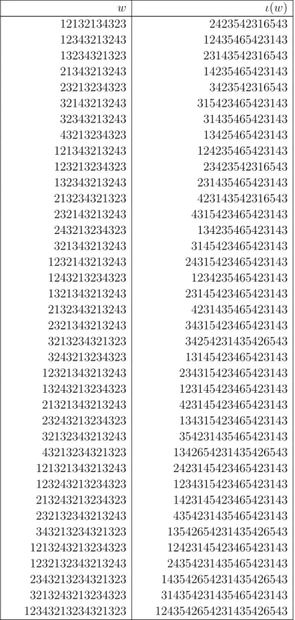
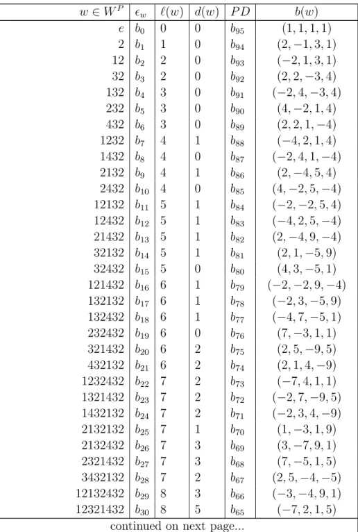
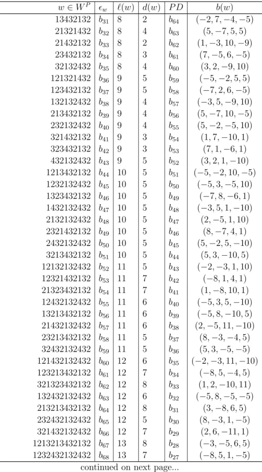
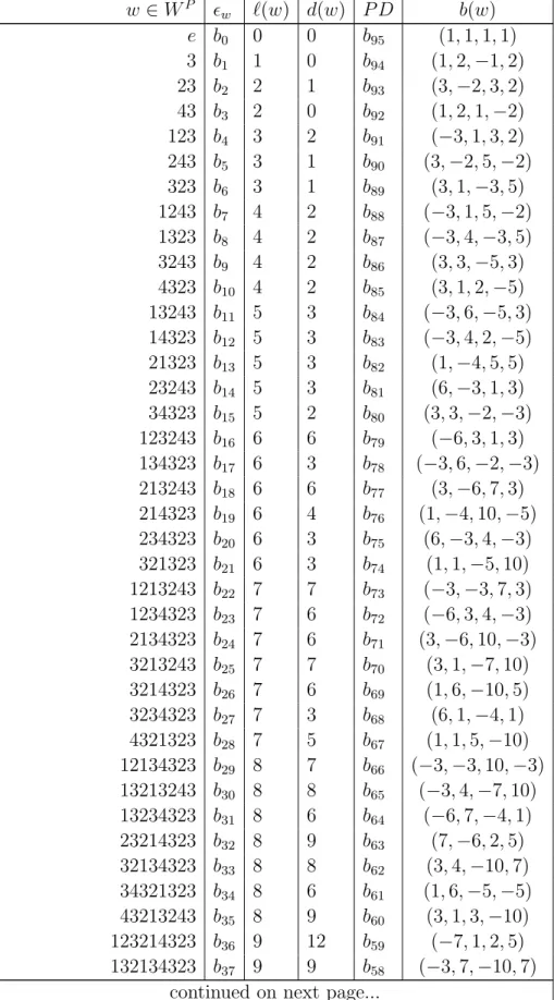
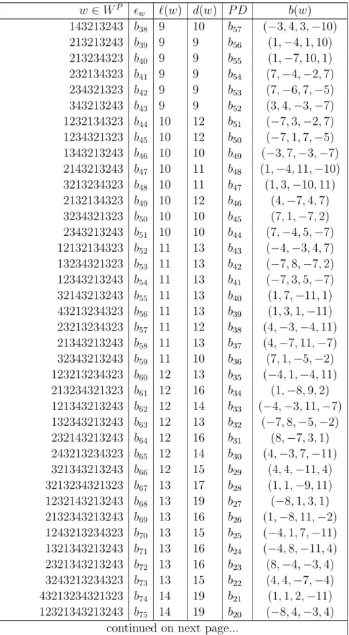
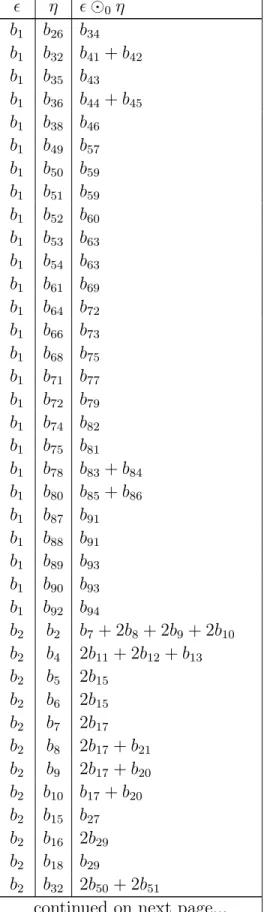
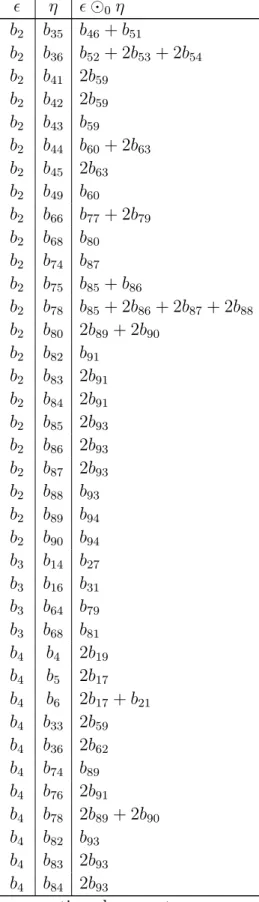
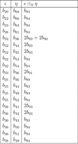
In these tables, a string of numbers of the formi1i2· · ·il is shorthand for the Weyl group element si1si2· · ·sil and e denotes the identity element of the Weyl group.

Table 1. WP˜1 _→_WP1 _{mapping for (}_{G2, D4}₎

˜

w w=ι( ˜w)

e e

1 1

21 21

121 3421

2121 23421

12121 123421

Table 2. WP˜2 _→_WP2 _{mapping for (}_G 2, D4)

˜

w w=ι( ˜w)