CAUSAL INFERENCE WITH PARTIAL INTERFERENCE AND RIGHT CENSORED OUTCOMES
Sujatro Chakladar
A dissertation submitted to the faculty of the University of North Carolina at Chapel Hill in partial fulfillment of the requirements for the degree of Doctor of Philosophy in
the Department of Biostatistics in the Gillings School of Global Public Health.
Chapel Hill 2018
Approved by:
Michael G. Hudgens Chirayath M. Suchindran Jianwen Cai
ABSTRACT
Sujatro Chakladar: Causal Inference with Partial Interference and Right Censored Outcomes
(Under the direction of Michael G. Hudgens)
Interference arises when the outcome of one individual depends on the treatment status of another individual. Partial interference is a special case of interference where individuals can be partitioned into groups such that no interference occurs between groups but may occur within groups. In the absence of interference, inverse probability weighted (IPW) estimators are commonly used to draw inference about causal effect. Tchetgen Tchetgen and VanderWeele (2012) proposed a modified IPW estimator for different causal effects in the presence of partial interference. An extension of the Tchetgen Tchetgen and VanderWeele IPW estimator is proposed for the setting where the outcome is subject to right censoring using inverse probability of censoring weights (IPCW). Censoring weights are calculated using parametric frailty models. The large sample properties of the IPCW estimators are derived and simulation studies are presented demonstrating the estimators’ performance in finite samples. The methods are illustrated using data from a cholera vaccination trial in Matlab, Bangladesh.
is proposed when there is time to event data with right censoring and possible partial interference. Parametric frailty models are used to model the probability of an event. Derivation of large sample properties of the estimator is provided. Simulation studies show the operating characteristics of the method for finite samples. The cholera vacci-nation trial in Matlab, Bangladesh is used to illustrate the methods in a real scenario.
ACKNOWLEDGEMENTS
This work was supported by NIH grant R01 AI085073. I would like to start by thanking my dissertation committee members for their valuable input and support. In particular, suggestions by Dr. Chirayath M. Suchindran and Dr. Stephen R. Cole about time dependent censoring and parametric frailty models have been instrumental in my project. I am also grateful to Dr. Jianwen Cai, especially for her recommendations on the finite sample behavior of my estimates. Finally, I am also thankful to Dr. Michael Emch for his comments that have made me appreciative about the implication of my method on real data and in turn, have helped a great deal to interpret the results of my work. Apart from my committee members, I would also like to thank Dr. M. Elizabeth Halloran for her comments and suggestions on my first paper.
During the course of my research work, I have often found myself lost trying to tackle problems both pertaining to my research work and my personal life. I am eternally grateful to my adviser Dr. Michael G. Hudgens for always helping me through those tough times. He has taught me a great deal about how to handle complex problems, being methodical, and research work in general. I regard him as a great teacher and I consider myself very fortunate to be one of his students. His unwavering motivation and support have made my research possible. I sincerely thank him for his guidance.
I would also like to thank my friends in North Carolina who have made my life here easier and friends outside of North Carolina who have enriched my world. In particular, to name a few, I am grateful towards Arkopal Choudhury, Arkaprava Roy, Aniket Bera, Suman Chakraborty, Sujayam Saha, Debraj Das, Pratyaydipta Rudra, Sayan Banerjee, Sayan Dasgupta, Abhishek Pal Majumder, Jyotishka Datta, Shalini Choudhury, Maxwell Datta, Subhamay Saha, Sapna Rao, Anwesha Goswami, Rinku Majumder, and Samarpan Majumder for always being there for me. I am thankful to Delilah for being in my life. Last but not the least, I am forever grateful to Sohini Raha for her unending support, constant enthusiasm, and for always guiding me through all the tough times that I encountered.
TABLE OF CONTENTS
LIST OF TABLES . . . x
LIST OF FIGURES . . . xi
CHAPTER 1: LITERATURE REVIEW . . . 1
1.1 Causal Inference . . . 1
1.1.1 Inverse Probability Weighting . . . 3
1.1.2 G Formula . . . 4
1.1.3 Doubly Robust Estimator . . . 4
1.2 Interference . . . 6
1.3 Censoring . . . 10
1.4 Motivating Data . . . 12
1.5 Summary . . . 13
CHAPTER 2: CAUSAL INFERENCE WITH PARTIAL INTERFERENCE AND RIGHT CENSORED OUTCOMES USING IPCW ESTIMATORS . . . 14
2.1 Introduction . . . 14
2.2 Methods . . . 15
2.2.1 Estimands . . . 15
2.2.2 Assumptions . . . 18
2.2.3 Proposed Estimator . . . 19
2.3 Simulation Study . . . 23
2.4.1 Cholera Vaccine Study and Analysis . . . 25
2.4.2 Results . . . 27
2.5 Discussion . . . 29
CHAPTER 3: PARAMETRIC G-FORMULA WITH PAR-TIAL INTERFERENCE AND RIGHT CENSORING . . . 35
3.1 Introduction . . . 35
3.2 Methods . . . 36
3.2.1 Estimands . . . 36
3.2.2 Assumptions . . . 39
3.2.3 Proposed Estimator . . . 40
3.3 Simulation . . . 46
3.4 Data . . . 48
3.4.1 Cholera Vaccine Study and Analysis . . . 48
3.4.2 Results . . . 50
3.5 Discussion . . . 52
CHAPTER 4: DOUBLY ROBUST ESTIMATION FOR DATA WITH PARTIAL INTERFERENCE AND RIGHT CENSORING . . . 58
4.1 Introduction . . . 58
4.2 Methods . . . 60
4.2.1 Estimands . . . 60
4.2.2 Assumptions . . . 63
4.2.3 IPCW and Parametric G Formula Estimators . . . 64
4.2.4 Proposed Estimator . . . 67
4.2.5 Properties of the Proposed Estimator . . . 68
4.3 Simulation . . . 74
4.4.1 Cholera Vaccine Study and Analysis . . . 78
4.4.2 Results . . . 81
4.5 Discussion . . . 82
CHAPTER 5: CONCLUSION . . . 91
APPENDIX A: TECHNICAL DETAILS FOR CHAPTER 2 . . . 93
APPENDIX B: TECHNICAL DETAILS FOR CHAPTER 3 . . . 95
APPENDIX C: TECHNICAL DETAILS FOR CHAPTER 4 . . . 97
LIST OF TABLES
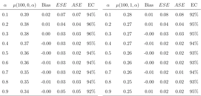
2.1 Results from simulation study described in Section 2.3. α denotes the allocation probability, µ(100, a, α) is the true
value of the target parameter fora= 0,1; Bias is the
aver-age ofµ(100, a, α)−µˆ(100, a, α)fora= 0,1; ESE is the
em-pirical standard error; ASE is the average of the sandwich variance estimates; and EC denotes the empirical coverage
of the 95% Wald confidence intervals. . . 34
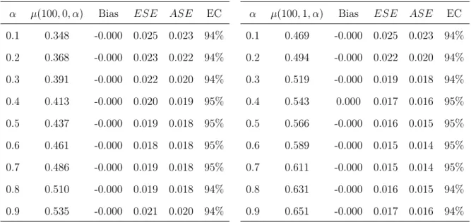
3.1 Results from simulation study described in Section 3.3. α denotes the allocation probabilities,µ(100, a, α)is the true
value of the survival probabilities at time point100fora= 0,1; bias is the average of µ(100, a, α)−mint(100, a, α,ωˆ),
ESE is the empirical standard error, ASE is the average of the sandwich variance estimators and EC denotes the
empirical coverage of the 95% Wald type confidence intervals. . . 56
3.2 AIC (BIC) values for different baseline hazard functions corresponding to gamma, inverse Gaussian and Positive
stable frailty distributions. . . 57
4.1 Results from simulation study described in Section 4.3. α denotes the allocation probabilities,µ(100, a, α)is the true
value of the target parameter for a = 0,1; Bias is the
av-erage of µ(100, a, α) − FˆDR(100, a, α) for a = 0,1; ESE
is the empirical standard error, ASE is the average of the sandwich variance estimates and EC denotes the empirical
coverage of the 95% Wald confidence intervals. . . 89
4.2 AIC (BIC) values for different baseline hazard functions corresponding to gamma, inverse Gaussian and positive
LIST OF FIGURES
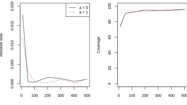
2.1 Absolute bias (left) and 95% confidence interval coverage
(right) for different numbers of groups for α = 0.5. The
dotted line in the right plot corresponds to95% coverage. . . 31
2.2 Estimated cumulative probability of cholera over time for vaccinated and unvaccinated for α = 0.3 (left), α = 0.45
(center) and α= 0.6 (right) . . . 32
2.3 Direct, indirect, total and overall effect estimates (×1000)
for different allocation strategies at time t = 1 year.
Indi-rect, total, and overall effects are with respect toα2 = 0.4. The shaded regions denote pointwise 95% confidence
inter-vals of the estimates. . . 33 3.1 Estimated cumulative probability of cholera against time
for vaccine and control forα= 0.3(left), α= 0.45(center)
and α= 0.6 (right) . . . 54
3.2 Direct effect, indirect effect, total effect and overall effect estimates multiplied by1000for different allocation
strate-gies at time t = 1 year. Indirect effects, total effects and
overall effects are with respect to α2 = 0.4. The shaded
region denotes the95% confidence interval of the estimates. . . 55
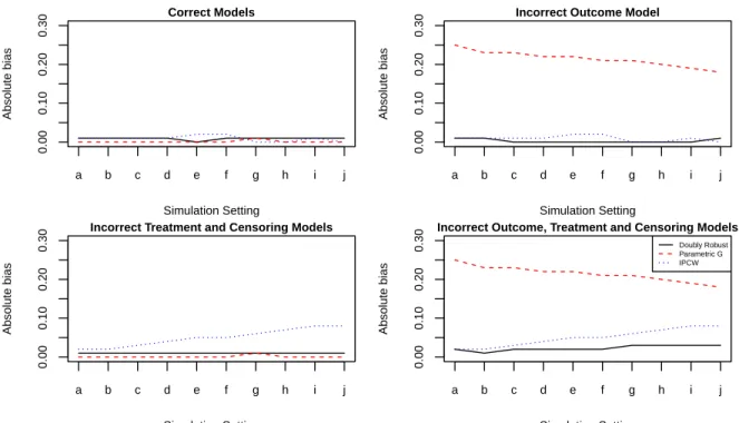
4.1 Absolute biases of the doubly robust, parametric g and the IPCW estimators under different model misspecifications
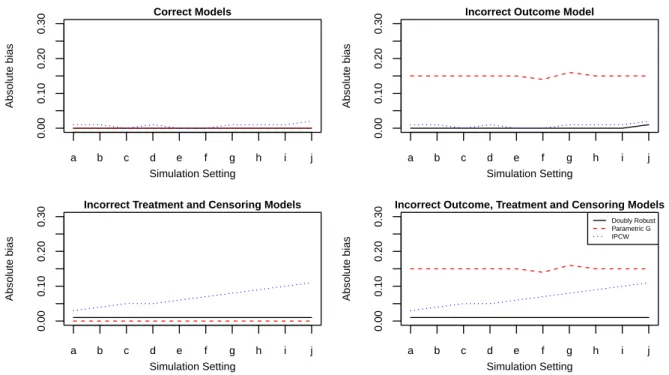
in control group. . . 84 4.2 Absolute biases of the doubly robust, parametric g and the
IPCW estimators under different model misspecifications
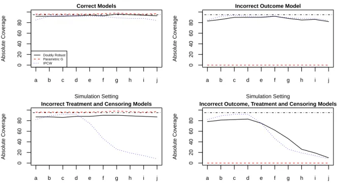
in treatment group. . . 85 4.3 Coverages of the doubly robust, parametric g and the IPCW
estimators under different model misspecifications in
con-trol group. . . 86 4.4 Coverages of the doubly robust, parametric g and the IPCW
estimators under different model misspecifications in
4.5 Direct effect, indirect effect, total effect and overall effect estimates multiplied by1000for different allocation
strate-gies at time t = 1 year. Indirect effects, total effects and
overall effects are with respect to α2 = 0.4. The shaded
CHAPTER 1: LITERATURE REVIEW
1.1 Causal Inference
Association does not always imply causation. Causal inference aims to address causal-ity in statistical inference. Splawa-Neyman et al. (1923) put forward the idea of potential outcomes which has become a building block of causal inference. Potential outcomes or counterfactual outcomes are defined to be all possible outcomes for a study which are not necessarily observed and can be treated as missing data. For example, consider a randomized clinical trial with a vaccine and a placebo. Then, the outcome when an indi-vidual would be administered placebo is not observed if the indiindi-vidual was administered treatment. This gives rise to the concept of potential outcomes or counterfactuals. In terms of mathematics, denote by Yi (i = 1, . . . , n), the binary outcome of n
individu-als. Ai represents the binary treatment status of individual i. Ai equals zero if the i-th
individual receives placebo and equals one if said individual receives treatment. The potential outcome for individualiunder treatmentais denoted byYia. So, if individuali receives placebo thenYi =Yi0 andYi1 is unobserved and if individualireceives treatment
then Yi = Yi1 and Yi0 is unobserved. This is termed to be causal consistency formally
defined first in Gibbard and Harper (1976) and discussed in detail by Cole and Frangakis (2009). Applications of this representation can be found in various literature including (Haavelmo 1944, Robins and Greenland 1996, Pratt and Schlaifer 1988), epidemiology (Greenland and Robins 1986, Robins et al. 2000; 1992, Robins 2000) social and behav-ioral sciences (Sobel 1990; 1995, Willkinson 1999) and statistics (Rubin 2004, Pratt and Schlaifer 1984).
For example, the average causal effect is defined as E(Y1)−E(Y0). He extended the ideas for randomized experiments to non randomized studies. Most of the causal inference framework assumes the Stable unit treatment value assumption (SUTVA) put forth by Rubin (1980). The assumptions
are-1. There is no interference between individuals. That is, the treatment status of one individual in no way affects the outcome of another individual. Mathematically Ai
has no effect onYj if i6=j.
2. There is only one version of treatment and control.
Along with SUTVA, in the case of a conditional randomized experiment or in an obser-vational setting, it is often assumed that given a set of measured covariates, the potential outcomes are independent of treatment. Denoting the set of measured confounders byL, this assumption can be represented as Ya ⊥⊥ A|L. This assumption is often referred to as conditional exchangeability (Hernán and Robins (2006), Hernan and Robins (2010)). Conditional exchangeability fails when there exist unmeasured covariates affecting both the treatment and outcome. Hence this assumption is also known as no unmeasured confounding. Another assumption that is often found in causal literature is the assump-tion of positivity discussed by Westreich and Cole (2010). According to this assumpassump-tion,
Pr(A= a|L =l) >0 for a ∈ (0,1) when Pr(L= l) >0. i.e. if a particular value of the
1.1.1 Inverse Probability Weighting
The idea of inverse probability weighting revolves around creating a pseudo population of individuals by weighting the study population with appropriate weights. The earliest known use of these IPW type estimators were suggested by Horvitz and Thompson (1952). These estimates have been used to estimate various causal effects like the average causal effect. For example, the IPTW estimate of E(Ya) is given to be
1
n
n X
i=1
I(Ai =a)Yi Pr(Ai =a|Li)
The weight for individual i is I(Ai=a)
Pr(Ai=a|Li). The assumption of positivity ensures that
1.1.2 G Formula
The generalized computation algorithm formula (g formula) provides an alternative way to compute causal effects and is free from the aforementioned drawback of IPW estimators discussed in the previous section. Robins (1986) proposed the g formula to estimate causal effects. Using parametric outcome regression models along with the g formula gives rise to the parametric g formula. This method is a generalization of stan-dardization (Hernán and Robins 2006). The assumptions discussed previously facilitate writing E(Ya) as being equal to ´ E(Y|A = a,L = l)dF
L(l). Again, the positivity assumption ensures that the parameter is well defined. So, an estimate of this causal quantity of interest Eˆ(Ya) is obtained by empirically estimating the distribution of L.
The form of the estimator is given as
follows-1
n
n X
i=1
ˆ
E(Y|A=a,Li)
ˆ
E(Y|A = a,Li) is estimated using an outcome regression model. For example, in case of a binary outcome, a logit model might be appropriate for modeling Y conditional on A and L. Parametric g formula has been proven to be particularly useful in adjusting for time varying confounders for time to event data (Young et al. 2011). Parameters of interest such as risk ratio (Taubman et al. 2009, Garcia-Aymerich et al. 2013, Cole et al. 2013) and hazard ratio (Westreich et al. 2012, Keil et al. 2014) have been calculated using this method. In all of these papers, pooled Logistic regression is the choice of parametric outcome model.
1.1.3 Doubly Robust Estimator
et al. 2008, Cole and Hernán 2008). Similarly if the outcome model is specified incorrectly then the estimates obtained using the parametric g formula can not be trusted (Taubman et al. 2009). The doubly robust estimator incorporates robustness within the estimator in the sense that the doubly robust estimator will generate reasonable results even when only one of the treatment and outcome regression models are specified correctly. Doubly robust estimators have existed in literature for sample survey data (Cassel et al. 1977, Särndal et al. 2003). There have been a number of papers on doubly robust estimators applied for the missing data problem and causal inference (Kang and Schafer 2007, Bang and Robins 2005). Lunceford and Davidian (2004) put forth a doubly robust estimator for estimating causal effects. The estimator proposed was a weighted combination of the IPW estimator and the parametric g estimator. The estimator is as follows
˜
E[Y1] =n−1
n X
i=1
AiYi− {Ai−Pr(ˆ Ai =a|Li)}mˆ1(Li)
ˆ
Pr(Ai =a|Li)
and
˜
E[Y0] =n−1
n X
i=1
(1−Ai)Yi+{Ai−Pr(ˆ Ai =a|Li)}mˆ0(Li)
1−Pr(ˆ Ai =a|Li)
1.2 Interference
Interference is said to be present in a data when the the treatment status of one indi-vidual affects the outcome of another indiindi-vidual (Cox 1958). An example of this might be data on infectious diseases. In this setting, whether a person gets infected or not might be affected by the treatment status of another individual (Halloran and Struchiner 1991). Partial interference is a special case of interference. Partial interference occurs when we have a partition of the data such that interference is observed within the individuals of a group but not between the individuals in different groups (Sobel 2006). Data might show traits of partial interference if there is a clear demographic separation between groups of individuals based on geography, society, or temporality. Therefore, interference can introduce possible indirect effects of interest which are termed spillover effects, or peer effects. These effects have been discussed in various fields including criminology (Samp-son 2010, Verbitsky-Savitz and Raudenbush 2012), developmental psychology (Duncan et al. 2005, Foster 2010), econometrics (Sobel 2006, Manski 2013), education (Hong and Raudenbush 2006, Vanderweele et al. 2013), imaging (Luo et al. 2012), political science (Sinclair et al. 2012, Bowers et al. 2013), social media and network analysis (VanderWeele and An 2013, Toulis and Kao 2013), (Eckles et al. 2014, Kramer et al. 2014), sociology (Aronow and Samii 2017), and spatial analyses (Zigler et al. 2012, Graham et al. 2013). Various literature propose methods for calculating interference effects in a randomized setting (Rosenbaum 2007, Hudgens and Halloran 2008, Baird et al. 2018, Eckles et al. 2016). Hudgens and Halloran (2008) presented estimands of direct, indirect, total and overall effects and proved the relations between them which was first discussed by Hallo-ran and Struchiner (1991). Modifying previous notation, suppose data now hasmgroups of individuals, withni individuals per group fori= 1, . . . , m. Denote by Aij, the
indica-tor of treatment status of individual j in group i i.e., if individual j in group i receives treatment thenAij = 1and otherwiseAij = 0. Also, let the vector of treatment indicator
Ai,−j. So, Ai = (Ai1, Ai2, ..., Aini) and Ai,−j = (Ai1, Ai2, ..., Aij−1, Aij+1..., Aini). Assume that possible realizations of Ai and Ai,−j are denoted by ai and ai,−j respectively. The outcome of individual j in group i is denoted by Yij (i = 1, . . . , m, j = 1, . . . , ni). The
potential outcome for individual j in group i under treatment a for the individual and treatment vector ai,−j for the rest of the individual in group i is denoted byYij(a,ai,−j).
Since there are only two versions of treatments, if there are n individuals in a group, then the set of all possible group treatment assignments consist of 2n elements and that
set is denoted by A(n) for n= 1,2, . . .. The vector of covariates for subject j in group i is denoted byLij and the matrix of covariates for all subjects in groupiis denote by Li,
i.e. Li = (Li1,Li2,· · · ,Lini). Hudgens and Halloran (2008) defined individual average potential outcome to be
¯
Yij(a, α) =
X
ai,−j∈A(ni−1)
Yij(a,ai,−j)π(ai,−j, α)
and the marginal individual average potential outcome to be
¯
Yij(α) = X
ai∈A(ni)
Yij(ai)π(ai, α)
where α denotes the group allocation strategies (Hong and Raudenbush 2006, Sobel 2006, Tchetgen and VanderWeele 2012, Hudgens and Halloran 2008). Specifically, ac-cording to the “Bernoulli" treatment allocation strategy discussed in Tchetgen Tchetgen and Vanderweele (2012) α can be interpreted as the probability with which an individ-ual receives treatment independently of others. Also, π(ai,−j, α) denote the conditional
probability that the treatment assignment for the ith group except for the jth individual
is ai,−j given that the jth individual in the ith group receives treatment a under
π(ai,−j, α) = Πkn=1i ,k6=jα
aik(1−α)1−aik. Similarly, letπ(a
i, α)denote the conditional
prob-ability that the treatment assignment for the ith group is a
i under allocation strategyα.
In terms of probability, π(ai, α) = Pr(Ai =ai). Then, π(ai, α) = Πnki=1αaik(1−α)1
−aik. The population average potential outcome is defined as
µ(a, α) =E
(
n−i 1
ni
X
j=1
¯
Yij(a, α) )
and the marginal population average potential outcome is defined as
µ(α) = E
(
n−i 1
ni
X
j=1
¯
Yij(a, α) )
Then, according to Halloran and Struchiner (1995) and Hudgens and Halloran (2008) the population average direct causal effect is a measure of the direct difference in effects between vaccinated and unvaccinated individuals. It is given by µ(0, α)−µ(1, α). The
population average indirect casual effect is a measure of the herd spillover effect and is the difference between the outcome of two unvaccinated individual under two different allocation strategies. It is given byµ(0, α1)−µ(0, α2)for allocation strategies α1 and α2. Population average total effect is a combination of both the direct and the indirect effects. It is obtained by taking the difference between the population average potential outcome of untreated individual at allocation level α1 and treated individuals at allocation level α2, i.e. µ(0, α1)−µ(1, α2). Finally population average overall effect is obtained by taking the difference between the average potential outcomes of individuals at allocation level α1 and individuals at allocation level α2, i.e. µ(α1)−µ(α2). If there is no interference present, then the direct effect would be equal to the total effect and the indirect effect would be 0. A two stage stratified interference method is applied and unbiased estimates of the parameters and also the variance estimator given the first stage of randomization is obtained given various assumptions.
might be ethical issues in implementing treatments selectively to randomized individuals. Tchetgen Tchetgen and VanderWeele (TV) (2012) suggested using inverse probability weighted (IPW) estimators for causal effects for observational data in such cases when partial interference might be present within the data. The estimators were constructed using group propensity scores instead of individual propensity scores. Perez-Heydrich et al. (2014) and Liu et al. (2016) showed large sample properties of these estimates. The estimate for the group level average potential outcome and marginal group level average potential outcome are given respectively by
ˆ
YiT V(a, α) =n−i1
n X
j=1
π(Ai,−j;α)I(Aij =a)Yij Pr(Ai|Li)
and
ˆ
YiT V(t, α) =n−i1
n X
j=1
π(Ai;α)Yij Pr(Ai|Li)
Using the estimators proposed by Tchetgen and VanderWeele (2012), Perez-Heydrich et al. (2014) went on to calculate group propensity scores via modeling the probability of participation using a mixed effects model. Using estimating equation representation and results from Stefanski and Boos (2002), asymptotic variance estimators were calculated and their estimators were given.
Liu et al. (2018) extends doubly robust estimators to the case with partial interference. The form of the group average potential outcome estimate is as
follows-ˆ
YiDR(a, α) = n−i 1
ni
X
j=1
[I(Aij =a){Yij(Ai)−mij(Ai, Lij, ˆ
β)}π(Ai,−j;α) Pr(Ai|Li,ωˆ)
+X
ai,−j
mij(a,ai,−j, Lij,βˆ)π(ai,−j;α)]
1.3 Censoring
In settings where the outcome of interest is survival time (e.g., time until infection), the outcome is typically subject to (right) censoring due to study completion or par-ticipant drop-out. Various semi parametric and parametric methods has been explored in order to analyze clustered survival data. Glidden and Vittinghoff (2004) provides a comparison of various methods of formulating the hazard function. Holt and Prentice (1974) put forth a stratified Cox model with hazard function gij(.) having the following
form
gij(t|Lij) =g0i(t) exp (LTijγ),
where the group specific baseline hazards g0i(.) are completely unspecified. Multiple
failure times for a single subject, which can be interpreted as correlated survival data, has also been analyzed using this method and the asymptotic properties of the estimator have been provided (Wei et al. 1989). However, this did not facilitate between group comparisons and Holt and Prentice (1974) suggested separate parameters to be estimated for the different groups, i.e.,
gij(t|Lij) = ξig0(t) exp (LTijγ),
Specifically, the authors considered the model corresponding to g0(t) = 1 (exponential) and g0(t) = tη−1. Pankratz et al. (2005) considered adding a random effect or frailty term ei keeping the baseline hazard unspecified as follows
gij(t|Lij) = g0(t) exp (LTijγ+ei).
the survival literature for analyzing correlated data use Bayesian techniques (Clayton 1991) like Gibbs sampling (Gauderman and Thomas 1994, Korsgaard et al. 1998), and Monte-Carlo EM algorithm (Li and Thompson 1997); and frequentist approaches (Li and Zhong 2002) like penalized likelihood maximization (Therneau et al. 2003).
Parametric frailty models have also been used to draw inference about right censored correlated data (Lancaster 1979, Hougaard 1984). Gutierrez et al. (2002) gives a detailed description of the various use of parametric frailty model in literature for analyzing right censored data. The general form of the parametric frailty model is given by
gij(t|Lij, ei) =g0(λ, t)eiexp (LTijγ)
where g0 is the baseline hazard function, λ is the parameter of the baseline hazard function, ei is a random component following density fe(ei;θr), t is the time to event
and γ is the vector of coefficients (Munda et al. 2012). The baseline hazard function is assumed to have a parametric form. Various distributions like exponential, Weibull etc. are used as the distribution of baseline hazard. The random component is known as the frailty term.
1.4 Motivating Data
A good motivating example for data with interference and right censoring is the cholera vaccine study in Matlab from a cholera vaccine trial in Matlab, Bangladesh (Ali et al. 2005). The data from this study were from children between the ages of 2 and 15 and women. The range of years through which data were collected was from 1985 to 1988. There were three available treatment groups and all the participants were randomized to one of these three groups. These treatment groups are B subunit-killed whole-cell oral cholera vaccine, killed whole-cell-only cholera vaccine and E. coli K12 placebo. The two vaccines were considered the same here for analysis purposes. The inclusion of a participant was subject to the condition that the individual received two or more doses of the vaccine. Non-participants were tracked using a vector of participation. The participation vector comprised of indicators of participation fro each individual. The vaccine and placebo were given from January 1985 to May 1985. Three centers were set up in the Matlab area for administering the dosages and all centers were used as surveillance centers as well. A total of 121,982 individuals were included. Perez-Heydrich et al. (2014) have shown in their paper that interference is present. Related individuals lived in clustered sets of houses called baris. There were a total of 6,415
baris. Demographic separation was used to categorize all the baris in the study to different groups (neighborhoods). The total number of these neighborhoods were prespecified to be
700. The assumption of partial interference treated these neighborhoods as groups such
that cholera can be transmitted from one individual to another within a neighborhood but not between individuals of two separate neighborhoods. Studies discovered that the probability of cholera among unvaccinated individuals was less for the neighborhoods with higher vaccination coverage (Ali et al. 2005, Emch et al. 2006).
period, migrated elsewhere from the study location or died during the follow up period.
1.5 Summary
CHAPTER 2: CAUSAL INFERENCE WITH PARTIAL INTERFERENCE AND RIGHT CENSORED OUTCOMES USING
IPCW ESTIMATORS
2.1 Introduction
Interference arises when the outcome of one individual depends on the treatment sta-tus of another individual (Cox 1958). For example, in the setting of infectious diseases, whether one individual receives a vaccine may affect whether another individual becomes infected (Halloran and Struchiner 1991). Partial interference is a special case of inter-ference where individuals can be partitioned into groups such that interinter-ference does not occur between individuals in different groups but may occur between individuals in the same group (Sobel 2006). Partial interference might be a reasonable assumption if groups of individuals are sufficiently separated geographically, socially, and/or temporally. Ef-fects due to interference, also known as spillover efEf-fects or peer efEf-fects, are of interest in many areas, including criminology (Sampson 2010, Verbitsky-Savitz and Raudenbush 2012), developmental psychology (Duncan et al. 2005, Foster 2010), econometrics (Sobel 2006, Manski 2013), education (Hong and Raudenbush 2006, Vanderweele et al. 2013), imaging (Luo et al. 2012), political science (Sinclair et al. 2012, Bowers et al. 2013), social media and network analysis (VanderWeele and An 2013, Toulis and Kao 2013, Kramer et al. 2014, Eckles et al. 2014), sociology (Aronow and Samii 2017), and spatial analyses (Zigler et al. 2012, Graham et al. 2013).
or individuals to different treatment or exposure conditions. In the observational setting, Tchetgen Tchetgen and VanderWeele (henceforth TV) (2012) proposed inverse probabil-ity weighted (IPW) estimators for different types of causal effects when there may be partial interference. Large sample properties of these IPW estimators were considered by Perez-Heydrich et al. (2014) and Liu et al. (2016).
In settings where the outcome of interest is a time to event, the outcome may be subject to right censoring due to study completion or participant drop-out. In the absence of interference, censoring is often accommodated by using inverse probability of censoring weights along with inverse probability treatment weights (Robins et al. 2000, Hernán et al. 2000, Robins and Finkelstein 2000, Cole and Hernán 2008, Cain and Cole 2009, Howe et al. 2011). In this section, an extension of the TV IPW estimators is considered for the setting where there may be partial interference and the outcome is subject to right censoring using inverse probability of censoring weights (IPCW).
The outline of this section is as follows. The proposed methods are developed in Section 2.2. In Section 2.3 simulation results are presented demonstrating the empirical performance of the proposed methods in finite sample settings. In Section 2.4 the meth-ods are used to analyze a cholera vaccine study of over 90,000 individuals in Matlab, Bangladesh. Section 2.5 concludes with a discussion.
2.2 Methods
2.2.1 Estimands
Suppose data are observed frommgroups of individuals, withniindividuals per group
for i = 1, . . . , m. Let Aij = 1 if individual j in group i receives treatment and Aij = 0
otherwise. Let Ai = (Ai1, Ai2, ..., Aini)and Ai,−j = (Ai1, Ai2, ..., Aij−1, Aij+1..., Aini). Let ai and ai,−j denote possible realizations of Ai and Ai,−j, and let A(n) denote the set of
fact, group i receives treatment ai by Tij(ai). The notation Tij(ai) reflects the partial
interference assumption, i.e., the potential outcome of individual j in group i does not depend on the treatment of individuals outside group i. Below the notation Tij(a,ai,−j)
is sometimes used to make explicit the treatment for individual j and the treatment for all other individuals in group i. Let Ti(.) = {Tij(ai) : ai ∈ A(ni), j = 1,2,· · · , ni}
denote the set of all potential event times for individuals in group i. Suppose the event times are subject to right censoring, e.g., due to loss to follow-up or study completion. Let Cij denote the potential censoring times for individual j in group i. Assume that
treatment has no effect on the censoring times, i.e., Cij does not depend on ai. Let ∆ij = 1 if Tij(Ai)≤Cij and ∆ij = 0 otherwise, and let Xij = min(Tij(Ai), Cij). Define
Xi = (Xi1, Xi2,· · · , Xini) and ∆i = (∆i1,∆i2,· · · ,∆ini). Denote by Lij the vector of baseline covariates for subject j in group i and by Li, the baseline matrix of covariates
for all subjects in groupi, i.e., Li = (Li1,Li2,· · · ,Lini). The group sizes ni are assumed to be random variables included in the baseline covariatesLij. Assume that themgroups
are randomly sampled from an infinite superpopulation of groups such that the observed data are m i.i.d. copies of Oi = (Li,Ai,Xi,∆i).
In the absence of interference, treatment effects are typically defined as contrasts in mean potential outcome for different counterfactual scenarios, e.g., the average treatment effect is usually defined as the difference in the mean potential outcomes had all individu-als received treatment versus had no individuindividu-als received treatment. Similarly, in the set-ting where there is partial interference, causal effects may be defined as contrasts in mean potential outcomes for different counterfactual scenarios (Hong and Raudenbush 2006, Sobel 2006, Hudgens and Halloran 2008, Tchetgen and VanderWeele 2012). Here we con-sider counterfactual scenarios where the marginal probability that an individual receives treatment, Prα(Aij = 1), equals α for different values of α∈ (0,1). The notation Prα(·)
described in TV is considered wherein individuals independently select treatment with probabilityα. Letπ(ai, α)denote the probability that groupireceives treatmentaiunder
Bernoulli allocation strategyα. That is,π(ai, α) = Prα(Ai =ai) = Qnk=1i αaik(1−α)1−aik.
Similarly let π(ai,−j, α) = Prα(Ai,−j =ai,−j|Aij =a) =Qnk=1i ,k=6 jαaik(1−α)1 −aik.
The causal estimands of interest defined below are contrasts in the risk of having an event by time t for different combinations of treatmenta and allocation strategies α. To define these estimands, let
¯
Fij(t, a, α) =
X
ai,−j∈A(ni−1)
I{Tij(a,ai,−j)≤t}π(ai,−j, α),
and
¯
Fij(t, α) = X
ai∈A(ni)
I{Tij(ai)≤t}π(ai, α).
In words, F¯ij(t, a, α) is the probability that individual j in group i will have an event
by time t when receiving treatment a and the group adopts policy α. Likewise, F¯ij(t, α)
is the probability that individual j in group i will have an event by time t when the group adopts allocation strategy α. Denote the group average risks by F¯i(t, a, α) =
n−i 1Pni
j=1F¯ij(t, a, α) and F¯i(t, α) = n−i 1 Pni
j=1F¯ij(t, α). Let µ(t, a, α) = Eα{F¯i(t, a, α)}
andµ(t, α) =Eα{F¯i(t, α)}whereEα{.}denotes the expected value under the
counterfac-tual setting when policy α is adopted in the super population of groups. In the cholera vaccine study described in Section 2.4, µ(t, a, α) denotes the average risk of acquiring
cholera by time t when an individual receives treatment a and other individuals receive vaccine with probability α. Various effects of treatment can be defined by contrasts in µ(t, a, α) and µ(t, α). The direct effect is obtained by comparing the probability of an
event when an individual receives treatment versus when not receiving treatment for a fixed allocation strategy. In particular, the direct effect at timetcorresponding to policy α is defined to be DE(t, α) = µ(t,0, α)−µ(t,1, α). The indirect (or spillover) effect
the individual does not receive treatment. Specifically, the indirect effect is given by IE(t, α1, α2) = µ(t,0, α1)−µ(t,0, α2) for allocation strategies α1 and α2. An indirect effect can analogously be defined when an individual is vaccinated. The total effect is defined as the difference between the probability of an event by timetwhen an individual does not receive treatment under policy α1 and when an individual receives treatment under policyα2, i.e., T E(t, α1, α2) =µ(t,0, α1)−µ(t,1, α2). Finally, the overall effect is the difference between the probability of an event by time t for policy α1 versus α2, i.e., OE(t, α1, α2) = µ(t, α1)−µ(t, α2).
2.2.2 Assumptions
Assume the following for all ai ∈ A(ni),
I) Conditional independence: Ai ⊥⊥Ti(.)|Li,
II) Positivity: Pr(Ai =ai|Li =l)>0for allai ∈ A(ni)andlsuch thatPr(Li =l)>0,
III) Conditional independent censoring: Ci ⊥⊥ {Ti(.),Ai}|Li.
Assumption I states that the potential event times for individuals within the same
group are conditionally independent of the actual treatment received by the group given covariates; this is a group-level generalization of the usual individual-level no unmeasured confounders assumption often made in the absence of interference. Positivity assumes that each group has a non-zero probability of being assigned every possible treatment combination given covariates for the group. Assumption III states that the potential
2.2.3 Proposed Estimator
In the absence of censoring, the IPW estimator proposed by TV can be used to draw inference aboutµ(t, a, α)andµ(t, α). In particular, lettingYij =I(Xij ≤t), the TV IPW
estimators areµˆT V(t, a, α) =m−1Pmi=1FˆiT V(t, a, α)andµˆT V(t, α) =m−1Pmi=1FˆiT V(t, α)
where
ˆ
FiT V(t, a, α) =n−i 1
ni
X
j=1
π(Ai,−j;α)I(Aij =a)Yij Pr(Ai|Li,βˆ)
, FˆiT V(t, α) =n−i 1
ni
X
j=1
π(Ai;α)Yij Pr(Ai|Li,βˆ)
,
and βˆis an estimator of the vector of parameters for the propensity model Pr(Ai|Li,β).
Details of the propensity model are discussed in the next sections.
In the presence of censoring, the following extension of the TV IPW estimators is proposed: µˆ(t, a, α) = m−1Pm
i=1Fˆi(t, a, α) and µˆ(t, α) =m−1 Pm
i=1Fˆi(t, α)where
ˆ
Fi(t, a, α) = n−i 1 ni
X
j=1
π(Ai,−j;α)I(Aij =a)I(∆ij = 1)I(Xij ≤t) Pr(Ai|Li,βˆ) Pr(∆ij = 1|Li, Xij,γˆ)
,
ˆ
Fi(t, α) =n−i 1 ni
X
j=1
π(Ai;α)I(∆ij = 1)I(Xij ≤t) Pr(Ai|Li,βˆ) Pr(∆ij = 1|Li, Xij,γˆ)
,
and γˆ is an estimator of the vector of the parameters for the censoring model.
De-tails of the censoring model are discussed in the next sections. Estimates of the di-rect, indidi-rect, total, and overall effects are given by DEd(t, α) = ˆµ(t,0, α)−µˆ(t,1, α),
c
IE(t, α1, α2) = ˆµ(t,0, α1) − µˆ(t,0, α2), dT E(t, α1, α2) = ˆµ(t,0, α1) − µˆ(t,1, α2) and d
OE(t, α1, α2) = ˆµ(t, α1)−µˆ(t, α2).
Known Treatment and Censoring Distributions
proof of the proposition is given in Section 2.6.
Proposition 1. If Pr(Ai|Li)and Pr(∆ij = 1|Li)are known for all j = 1,2, . . . , ni, then
E{Fˆi(t, a, α)}= ¯Fi(t, a, α) and E{Fˆi(t, α)}= ¯Fi(t, α).
Unknown Treatment and Censoring Distributions
In observational studies, neither the conditional distribution of treatment given covariates nor the conditional distribution of censoring given covariates are known. Therefore, we consider finite dimensional parametric models to estimate the group propensity scores and conditional probability of censoring; these estimates are then plugged into the IPCW estimators defined above. The conditional probability of censoring is estimated using a frailty model (Munda et al. 2012) where the conditional hazard for Cij is assumed to
have the form gij(c|Lij, ei) = g0(c;θh)eiexp (LTijθc), where g0 is the baseline hazard function,θh is theq0- dimensional parameter vector of the baseline hazard function, ei is
a random effect with density fe(ei;θr), andθc is theq-dimensional vector of coefficients. Letγ= (θc,θh, θr)be the vector of parameters for the frailty model. Maximum likelihood
theory can be used to draw inference about γ. Under assumption III, the contribution of group i to the marginal log-likelihood is (Munda et al. 2012)
l(Xi,∆i,Li,γ) =
ni
X
j=1
∆ij
log{g0(Xij)}+LTijθc
+ (−1)diL(di)
ni
X
j=1
G0(Xij) exp (LTijθc),
where di = Pnj=1i (1 − ∆ij) is the number of censored observations in group i,
G0(ω) =
´ω
0 g0(κ)dκ, andL
(s) is thes-th derivative of the Laplace transform of the frailty distribution, i.e., L(s) = ´∞
estimator of γ solves the following estimating equations
X
i
ψck(Xi,∆i,Li,γ) = 0 for k= 1, ..., q+q0+ 1,
where ψck =ψck(Xi,∆i,Li,γ) = ∂l(Xi,∆i,Li,γ)/∂γk and γk is the k-th element of γ.
Below, the baseline hazard for the censoring model is assumed to be constant and equal to θh such that gij(c|Lij, ei) = θhexp (Lijθc)ei. In addition, the frailty term ei is
assumed to follow a gamma distribution with mean 1and variance θr. So, the censoring
weight for an uncensored individual equals
Pr(∆ij = 1|Li,γ) =
ˆ
Pr(Cij > Tij(Ai)|Li,γ, ei)fe(ei;θr)dei
=
ˆ
Pr(Cij > Xij|Li,γ, ei)fe(ei;θr)dei
=
ˆ
exp{−θhXijexp (Lijθc)ei}
e1/θr−1
i e
−ei/θr
θ1/θr
r Γ1/θr
dei
=
1
θrθhXijexp (Lijθc) + 1 1/θr
Following TV (2012), a mixed effects model may be assumed for the treatment allocation, i.e., Pr(Aij = 1|Lij, bi) = logit−1(Lijθx+bi)wherebi is a random effect following density
fb(bi;θs). (In the application below the mixed effects model has a slightly more
compli-cated form owing the particulars of the design of the study analyzed.) Let β = (θx, θs)
denote the(p+ 1)dimensional vector of parameters for the mixed effects model. Again,
maximum likelihood theory can be used to draw The contribution of group i to the log-likelihood for the mixed effects model is given by
l(Ai,Li,β) = log
"ˆ ni Y
j=1
hij(bi,Li,θx)Aij{1−hij(bi,Li,θx)}(1−Aij)fb(bi;θs) #
,
solution to the score equations
X
i
ψxk(Ai,Li,β) = 0 for k = 1, ..., p+ 1,
where ψxk =ψxk(Ai,Li,β) = ∂l(Ai,Li,β)/∂βk,βk is the k-th element of β.
Inference about the causal effects of interest is then based on solving the vector of estimating equations
X
i
ψ(Oi,θ) = 0, (2.1)
where θ = (γ,β, θ), ψ(Oi,θ) = (ψc,ψx, ψaα) T,
ψc = (ψc1, ψc2, ..., ψcq+q0+1)T , ψx =
(ψx1, ψx2, ..., ψxp+1)T ,
ψaα=ψaα(Oi,θ) =
g∗(Oi, a, α,γ) Pr(Ai|Li,β)
−θ,
and
g∗(Oi, a, α,γ) = n−i 1 n X
j=1
π(Ai,−j;α)I(Aij =a)I(Xij ≤t) Pr(∆ij = 1|Lij, Xij,γ)
.
Let θˆ = (γ,ˆ β,ˆ µˆ(t, a, α)) denote the solution to (1). Denote the true value of θ by θ0 = (γ0,β0, µ(t, a, α))and note that
ˆ
ψaα(o,γ0,β0, µ(t, a, α))dFO(o) =E
g∗(Oi, a, α,γ0)
Pr(Ai|Li,β0)
−µ(t, a, α)
= 0,
where FO denotes the joint distribution of the complete observed random variable O and the last equality follow from the Proposition above. Therefore, assuming the parametric models above are correctly specified, it follows that ´ ψ(o,θ0)dFO(o) =
0. By M-estimation theory (Stefanski and Boos 2002), θˆ →p θ0 and √
m( ˆθ − θ0) converges in distribution to a Normal distribution with mean 0 and covariance
normality of the direct, indirect and total effect estimators follows from the delta method. Similar techniques can be used to show that µˆ(t, α) and the overall effect estimator are
also consistent and asymptotically Normal. The asymptotic variance Σ can be consis-tently estimated by Σˆ = ˆU( ˆθ)−1Vˆ( ˆθ){Uˆ( ˆθ)−1}T where Uˆ( ˆθ) = m−1Pm
i=1{−ψ˙(Oi,θˆ)}
and Vˆ( ˆθ) = m−1Pm
i=1{ψ(Oi,θˆ)ψ(Oi,θˆ)T}. The empirical sandwich variance estimator ˆ
Σcan be computed using the R packagegeex(Saul and Hudgens 2017) and can be used
to construct Wald type confidence intervals (CIs).
2.3 Simulation Study
A simulation study was conducted to assess the finite sample bias of the IPCW esti-mator and coverage of the corresponding Wald confidence intervals. The data generating model used in the simulation study was motivated by aspects of the cholera vaccine study analysis presented in the next section. Following Perez-Heydrich et al. (2014), data were simulated according to the following steps.
i) First, two baseline covariates L1ij and L2ij were randomly generated. In the
ap-plication presented in Section 2.4, conditional exchangeability is assumed given an
individual’s age (in decades) and the distance of their residence to the nearest river. Motivated by this example,L1ij andL2ij were randomly generated as follows. First,
Vij was randomly generated from an exponential distribution with mean 20. Then
L1ij was set to min(Vij,100)/10. The second set of covariates L2ij were randomly
sampled such that logL2ij ∼normal(0,0.75).
ii) The random effects for the treatment modelbiwere randomly sampled from a normal
distribution with mean0 and variance 0.0859.
iii) The treatment indicators Aij were randomly sampled from a Bernoulli distribution
iv) The potential times to event Tij(ai) were randomly sampled from an exponential
distribution with meanµij = 200 + 100aij −0.98L1ij −0.145L2ij + 50Pk6=jaik/ni.
v) The random effects for the censoring model ei were randomly generated from a
gamma distribution with mean 1and variance θ = 1.25.
vi) Censoring times Cij were randomly sampled from an exponential distribution with
mean1/λ0 where λ0 = 0.015 exp (0.002L1ij + 0.015L2ij)ei.
vii) Individual censoring indicators were determined i.e., ∆ij = 0 if Cij < Tij(Ai).
Steps i through vii were used to stochastically generate 1000 data sets, with each data set containing 500 groups with 10 individuals per group. For each simulated data set, the IPCW estimator of µ(100, a, α) was evaluated for a= 0,1 and α = 0.1,0.2, . . . ,0.9.
Estimated standard errors based on the empirical sandwich variance estimator and Wald 95% confidence intervals were also calculated for each simulated data set. Empirical standard errors were calculated by taking the standard deviation of the point estimates from all simulations.
The true value of the estimand was obtained by simulating counterfactual outcomes form = 106groups of individuals. Note that, according to the model used to generate the data, potential survival times depend only on P
k6=jaik. So, µ(t, a, α) was approximated
by (Perez-Heydrich et al. 2014)
m−1
m X
i=1 n−i 1
ni
X
j=1
ni−1
X
k=0
ni−1
k
I{Tij(a, k)≤t}αk(1−α)ni−k−1.
The true value ofµ(t, α) was determined in a similar fashion.
Results from the simulation study are presented in Table 2.1. Bias of the IPCW estimator was negligible for all values of a and α. Likewise, the average estimated stan-dard error was close to the empirical stanstan-dard error. Coverage of the95% Wald CIs was
Additional simulation studies were conducted to assess the performance of the pro-posed methods for different values of m, the total number of groups, ranging from 10 to 500. The number of individuals per group was 10, as in the previous simulations. For each m∈ {10,50,100,200,300,400,500},1000data sets were simulated according to
steps i through vii above. Results are depicted in Figure 2.1. Bias of the IPCW estimator was small and coverage of the Wald CIs was close to the nominal level provided m was at least 50.
2.4 Data Analysis
2.4.1 Cholera Vaccine Study and Analysis
In this section, the methods described in Section 2.2 are used to analyze a cholera
vaccine study in Matlab, Bangladesh (Ali et al. 2005). Eligible study participants were children 2–15 years of age and women greater than 15 years old. All 121,975 eligible
individuals in the population were randomized to one of three vaccination groups: B subunit-killed whole-cell oral cholera vaccine, killed whole-cell-only cholera vaccine, and E. coli K12 placebo. As in Perez-Heydrich et al. (2014), no distinction is made between the two vaccines in the analysis presented here. Individuals were considered to have participated in the randomized trial component of the study if they received two or more doses of vaccine or placebo. The primary endpoint of the trial was incident cholera. Three health centers in the Matlab area served as surveillance centers and collected endpoint data on all individuals, regardless of whether they participated in the randomized trial. The analysis presented here includes data from all individuals, i.e., trial participants as well as those who chose not to participate. Thus an approach which accounts for possible confounding, such as the IPW method described in Section 2, should be utilized to assess the effects of vaccination.
for censoring. Here individuals are considered right censored if they were not diagnosed with cholera during the study. Individuals who emigrated from the study location or died during the follow-up period prior to cholera infection were right censored at the time of emigration or death. Individuals who did not emigrate or die and who did not develop cholera during the study were right censored at the end of the study period.
Related individuals in Matlab live in clustered sets of houses called baris. There were a total of 6,415 baris at the time of the vaccine trial. Perez-Heydrich et al. (2014) used a clustering algorithm to form groups (neighborhoods) based on the spatial location of the baris, with the number of groups pre-specified to be 700. The analysis here is based on the same groups as in Perez-Heydrich et al. and assumes that there is no interference between individuals in different groups, i.e, the vaccination of an individual in one group has no effect on whether an individual in another group acquires cholera. When fitting the propensity modelPr(Ai|Li,β)described below, the largest 15 groups had estimated
group propensity scores that were effectively equal to zero and therefore these groups were omitted.
Individuals participating in the vaccine trial were not all vaccinated on the same calendar day, such that the level of vaccine coverage within a group varied over a relatively brief period of calendar time at the study onset. For simplicity and because the methods developed above do not accommodate time varying treatment, the start of follow-up for all individuals in a particular group was set to the latest date of second vaccination among all individuals in that group. Some observations were excluded because individuals contracted cholera, died, or emigrated prior to the start of follow-up for their group.
As in Perez-Heydrich et al., the group propensity score was modeled using a mixed effects model. The particular form of the model derives from the fact that in order for an individual to have received a vaccine, they must have (i) chosen to participate in the trial, and (ii) been randomized to receive one of the two vaccines. To account for (i), a logistic regression model for participation was assumed. As in Perez-Heydrich et al., covariates in the participation component of the model were age, squared age, distance to nearest river, and squared distance to nearest river. Accommodating (ii) in the propensity model is straightforward because, due to randomization, individuals who elected to participate in the trial were known to receive one of the two vaccines with probability 2/3. Combining these two aspects of the model, the propensity score for group i was estimated by
Pr(Ai|Li,βˆ) =
ˆ
Π
nij=1{(2/3)hij(bi,Lij,θˆx)}Aij{1−(2/3)hij(bi,Lij,θˆx)}(1−Aij)
×fb(bi; ˆθs),
where hij(bi,Li,θx) = Pr(Bij = 1|bi,Lij,θx) = expit(Lijθx +bi), Bij is the indicator
of participation, i.e., Bij = 1 if individual j in group i participated in the randomized
trial and Bij = 0otherwise, and (θˆx,θˆs) is the maximum likelihood estimate of (θx, θs).
Censoring was modeled using the gamma frailty model described above, and only included age as covariate as no other variables were associated with censoring. Over 70% of
individuals belonged to groups where the vaccine coverage was between 0.3 and 0.6.
Therefore, the analysis was conducted for allocation strategies ranging from 0.3 to0.6.
2.4.2 Results
of interference. This decrease is more modest when an individual is vaccinated, indicating a stronger indirect effect when unvaccinated. At all time points the estimated risk of cholera is higher when an individual is unvaccinated, suggesting a beneficial, direct effect of vaccination, especially at lower coverage levels. For α = 0.3 and α = 0.45, the
estimated risk when unvaccinated increases suddenly between 200 and 300 days, and then again between 300 and 400 days. These results might be attributable to the known bimodal seasonality of cholera in Bangladesh (Longini et al. 2002). Note that, because the study start date varied across groups, the time scale in this analysis does not exactly coincide with calendar time. Nonetheless, 95% of individuals had a start date within a
two calendar month range, such that there is a strong correlation between the analysis time scale and calendar time, and thus cholera seasonality may explain these periods of marked increase in risk.
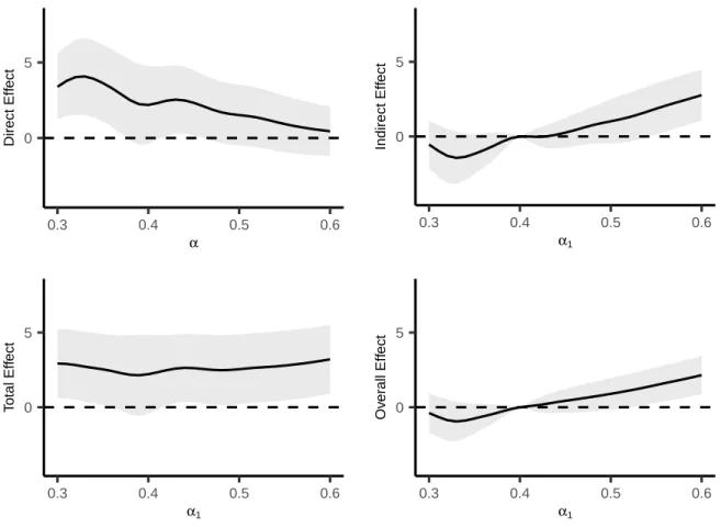
Direct, indirect, total and overall effect estimates and 95% CIs (×1000) for
differ-ent allocation strategies at time t = 1 year are shown in Figure 2.3. The direct effect
estimates generally decrease as α increases. For example, the direct effect estimate for α= 0.35is3.6 (95%CI1.1,6.2)whereas forα= 0.5the direct effect estimate is1.5 (95%
CI −0.5,3.5). The indirect, total, and overall effect estimates in Figure 2.3 compare the
cholera per 1000 individuals per year are expected if 60% of individuals are vaccinated
compared to if only 40% of individuals receive vaccine.
In previous analyses of these data, Perez-Heydrich et al. also estimated the direct, indirect, total and overall effects using a binary outcome indicating whether an individual was infected with cholera during the first year of follow-up. The IPCW estimates fort = 1
are similar to these previous results, e.g., Perez-Heydrich et al. estimated the direct effect for alpha=0.32 to be 5.3 (95% CI 2.5, 8.1) whereas the IPCW estimate of this effect at
t= 1is 4.0 (95%CI 1.6, 6.5). However,the Perez-Heydrich et al. estimates may be biased
because they did not account for right censoring.
2.5 Discussion
In this section, the TV IPW estimator for partial interference was extended to allow for right censored outcomes. The proposed estimator was obtained by weighting the original TV estimator by censoring weights calculated from a parametric frailty model of the censoring times. The estimator was shown to be consistent and asymptotically normal and a consistent estimator of the asymptotic variance was proposed. A simulation study demonstrated that the proposed methods performed well in finite samples provided the number of groups is sufficiently large. Analysis of a cholera vaccine study using the proposed methods suggests vaccination had both a direct and indirect effect against cholera infection. These results are in accordance with findings by Ali et al. (2005) and Perez-Heydrich et al. (2014), but are likely more accurate since these previous analyses did not formally account for right censoring.
Figure 2.1: Absolute bias (left) and95% confidence interval coverage (right) for different
numbers of groups for α = 0.5. The dotted line in the right plot corresponds to 95%
coverage.
0 100 200 300 400 500
0.000
0.005
0.010
0.015
0.020
Number of Groups
Absolute Bias
a = 0 a = 1
0 100 200 300 400 500
0
20
40
60
80
100
Number of Groups
Co
v
er
Figure 2.2: Estimated cumulative probability of cholera over time for vaccinated and unvaccinated for α= 0.3(left), α= 0.45 (center) and α= 0.6 (right)
0 100 300
0.000
0.004
0.008
0.012
Time (Days)
Cum
ulativ
e Probability of Choler
a
0 100 300
0.000
0.004
0.008
0.012
Time (Days)
0 100 300
0.000
0.004
0.008
0.012
Figure 2.3: Direct, indirect, total and overall effect estimates (×1000) for different
allo-cation strategies at timet = 1year. Indirect, total, and overall effects are with respect to
α2 = 0.4. The shaded regions denote pointwise 95% confidence intervals of the estimates.
0 5
0.3 0.4 0.5 0.6
α
Direct Eff
ect
0 5
0.3 0.4 0.5 0.6
α1
Indirect Eff
ect
0 5
0.3 0.4 0.5 0.6
α1
T
otal Eff
ect
0 5
0.3 0.4 0.5 0.6
α1
Ov
er
all Eff
α µ(100,0, α) Bias ESE ASE EC α µ(100,1, α) Bias ESE ASE EC
0.1 0.39 0.02 0.07 0.07 94% 0.1 0.28 0.01 0.08 0.08 92%
0.2 0.38 0.01 0.04 0.04 96% 0.2 0.27 0.01 0.04 0.04 95%
0.3 0.38 0.00 0.03 0.03 96% 0.3 0.27 -0.00 0.03 0.03 95%
0.4 0.37 -0.00 0.03 0.02 95% 0.4 0.27 -0.01 0.02 0.02 94%
0.5 0.36 -0.00 0.03 0.02 94% 0.5 0.26 -0.00 0.02 0.02 93%
0.6 0.36 -0.01 0.03 0.02 94% 0.6 0.26 -0.00 0.02 0.02 93%
0.7 0.35 -0.00 0.03 0.02 94% 0.7 0.26 -0.01 0.02 0.01 94%
0.8 0.35 -0.01 0.03 0.03 94% 0.8 0.25 -0.00 0.02 0.02 93%
0.9 0.34 -0.00 0.05 0.05 92% 0.9 0.25 0.01 0.02 0.02 95%
Table 2.1: Results from simulation study described in Section 2.3. α denotes the alloca-tion probability,µ(100, a, α)is the true value of the target parameter for a= 0,1; Bias is
the average ofµ(100, a, α)−µˆ(100, a, α)fora= 0,1; ESE is the empirical standard error;
CHAPTER 3: PARAMETRIC G-FORMULA WITH PARTIAL INTERFERENCE AND RIGHT CENSORING
3.1 Introduction
Interference is present when the outcome of one individual depends on the treatment status of another individual (Cox 1958). An example of this might be data on infectious diseases. For these types of data, whether a subject becomes infected or not might be affected by the vaccination status of another individual (Halloran and Struchiner 1991). Sobel (2006) introduces the notion of partial interference as a subset of interference. If individuals can be partitioned into groups such that interference can occur within individ-uals of one group but it cannot occur between individindivid-uals from two separate groups, the data is said to show traits of partial interference. Well defined social, temporal, and/or geographical difference between groups of people might be a valid reason for assuming they have partial interference. Interference might produce effects termed spillover effects or peer effects, which are of importance for various different fields of study.
the parametric g formula. The generalized computation algorithm formula (g formula) was first put forward by Robins (1986). G-formula, together with outcome regression produces the parametric g formula. The theory of parametric g formula is generalized from standardization (Hernán and Robins 2006). Parametric g formula has been used mainly in adjusting for time varying confounders for time to event data (Young et al. (2011)). Many authors used parametric g formula to calculate risk ratio (Taubman et al. (2009), Garcia-Aymerich et al. (2013), Cole et al. (2013)) and hazard ratio (Westreich et al. (2012), Keil et al. (2014)). However, all of the authors have used logistic regression for modeling the probability of outcome.
The rest of the section is organized as follows. Section 3.2 introduces the estimators and estimands. Results from simulation studies illustrating the finite sample behavior of the method are presented in Section 3.3. The proposed method is implemented on a real data consisting of 100,000 individuals in Matlab, Bangladesh in Section 3.4.
3.2 Methods
3.2.1 Estimands
Assume that there are m groups, each group having ni individuals in them for
i = 1, . . . , m. Depending on whether individual j in group i gets treatment or placebo, denote Aij = 1 or Aij = 0 respectively. Let Ai = (Ai1, Ai2, ..., Aini) and Ai,−j = (Ai1, Ai2, ..., Aij−1, Aij+1..., Aini) denote the overall group treatment assignment and the group treatment assignment without individual j for group irespectively. Also, let Ai and Ai,−j attain possible values ai and ai,−j respectively. The potential time to
event for individual j in groupiwith treatment ai is denoted byTij(ai). These potential
times exhibit traits of partial interference in the sense that the potential time to event Tij(ai) for individual j in group i might be dependent on the treatment status of
indi-vidual j0 in group i even when j0 does not equal j. However, if i 6= i0, then Tij(ai) is
iis denoted byTi(.) = {Tij(ai) :ai ∈ A(ni), j = 1,2,· · · , ni}. Assume that there is right
censoring within the time to events. Also assume that Cij are censoring time for
individ-ual j in group i. Let ∆ij =I(Tij(Ai) ≤ Cij) and Xij = min(Tij(Ai), Cij). Then ∆ij is
the censoring indicator and Xij is the observed time to event for individual j in group i.
The vector of censoring indicators for group i denoted by ∆i equals (∆i1,∆i2,· · · ,∆ini) and the vector of observed time to events denoted byXi equals(Xi1, Xi2,· · · , Xini). The set of every feasible 2n assignments of treatments for n = 1,2, . . . is denoted by A(n).
Finally, the vector of all the covariates for subject j in group i is termed as Lij and
Li = (Li1,Li2,· · · ,Lini) denotes the matrix of covariates for group i. Let the baseline covariates Lij include group sizes ni. The m groups in data is assumed to be sampled
from an infinite superpopulation of groups and the m observations (Li,Ai,Xi,∆i) are
i.i.d..
receives treatment a under allocation strategy α be denoted by π(ai,−j, α).
Mathemat-ically, this can be denoted as follows π(ai,−j, α) = Pr(Ai,−j = ai,−j|Ai,j = a). Then,
π(ai,−j, α) = Πnk=1i ,k6=jαaik(1−α)1
−aik. Similarly, letπ(a
i, α)denote the conditional
prob-ability that the treatment assignment for the ith group is a
i under allocation strategy
α. In terms of probability, π(ai, α) = Pr(Ai =ai). Then, according to the independent
Bernoulli probability assumption for α, π(ai, α) = Πnk=1i α
aik(1−α)1−aik.
The various contrasts in survival probabilities for different combinations of treatment and allocation strategies are possible causal estimands of interest. To properly introduce these estimands, first the following has to be defined,
¯
Fij(t, a, α) =
X
ai,−j∈A(ni−1)
I{Tij(a,ai,−j)≤t}π(ai,−j, α),
¯
Fij(t, α) = X
ai∈A(ni)
I{Tij(ai)≤t}π(ai, α),
¯
Fi(t, a, α) = n−i 1 Pni
j=1F¯ij(t, a, α) and F¯i(t, α) = n
−1
i Pni
j=1F¯ij(t, α). F¯i(t, a, α) can be interpreted as the average probability that an individual will fail by timetin groupiwhen the individual receives a and the group adopts allocation strategy α. Similarly, F¯i(t, α)
can be interpreted as the average probability that an individual will fail by time t in groupi when the group adopts allocation strategyα . Finally,µ(t, a, α) =E{F¯i(t, a, α)}
is the population average potential cumulative distribution at the point t for treatment a under allocation strategy α. Similarly µ(t, α) = E{F¯i(t, α)} is the population average overall potential cumulative distribution at the point t under allocation strategy α. A possible interpretation ofµ(t, a, α)might be as the probability of an individual’s survival
time being less thantunder the counterfactual case that an individual receives treatment a under allocation strategy α,. Again, a possible interpretation of µ(t, α) might be as
The various causal effects of interest are as follows. Comparison of the probability of event of treated individuals with untreated at a particular allocation level gives rise to direct effect. The population average direct effect at time t with the data having allocation probability α is given by DE(t, α) = µ(t,0, α) −µ(t,1, α). Subtraction of
the probability of event for two different levels of allocation among the untreated gives rise to the indirect effect. For allocation strategies α1 and α2, the population average indirect effect is then given by IE(t, α1, α2) = µ(t,0, α1)−µ(t,0, α2). The difference T E(t, α1, α2) = µ(t,0, α1)−µ(t,1, α2) is termed as the total effect. This is the difference between the probability of event of untreated individual at allocation levelα1and treated individuals at allocation levelα2. The final effect of interest to be discussed is the overall effect. The calculation of this involves subtracting the probability of event of individuals at allocation levelα1and individuals at allocation levelα2, i.e. OE(t, α1, α2) = µ(t, α1)− µ(t, α2).
3.2.2 Assumptions
The following assumptions are made:
I) Conditional independence: Ai ⊥⊥Ti(.)|Li,
II) Positivity: Pr(Ai =ai|Li =l)>0for allai ∈ A(ni)andlsuch thatPr(Li =l)>0,
III) Conditional independent censoring: Ci ⊥⊥ {Ti(.),Ai}|Li.
In the absence of interference, assumption I is a standard assumption made for each individual. When interference is present, this assumption is extended for the group in-stead of individuals. Under the no interference assumption, assumption (I) is referred
to as no unmeasured confounding. In this case, assumption (I)states that the observed
observed. Assumption II is termed as positivity. Given all possible values of the
mea-sured confounders, the positivity assumption states that given all possible values of the measured confounders, the probability of a group being assigned a particular vector of treatment combination is always positive. Assumption III is related to the censoring
distribution. This assumption proposes that the censoring time for an individual is con-ditionally independent of the counterfactual time to event under and the actual treatment assignment for the group when all the possible confounders are given.
3.2.3 Proposed Estimator
In the absence of interference and censoring, Hernán and Robins (2006) showed that standardization can be used to estimate risk ratios. The form of the standardized estimate of the counterfactual mean E(Ya)in this case is
m(a) =
ˆ
ˆ
E(Y|A=a,L=l)dFˆL(l)
or equivalently,
m(a) = 1
m
m X
i=1
1
ni ni
X
j=1
ˆ
E(Y|A=a,Lij)
where Y denotes the indicator that an individual has had an event till a specific time point of concern and FˆL denotes the empirical joint distribution of the covariates L. In
previous literature, logistic regression has often been used to estimate Eˆ(Y|A = a,Lij)
(Taubman et al. 2009) and authors had mainly focused on calculating risk ratios or hazard ratios. However, the parametric g formula might be extended for cases with time to event data and interference. The proposed estimator for the causal and survival quantities of interest µ(t, a, α) defined in Section3.2.1 is as
follows-mint(t, a, α,ωˆ) =
ˆ
X
ai,−k∈A(ni−1)