plasmonic near fields
Martín Caldarola, Biswajit Pradhan, and Michel Orrit
Citation: The Journal of Chemical Physics 148, 123334 (2018); doi: 10.1063/1.5023171
View online: https://doi.org/10.1063/1.5023171
View Table of Contents: http://aip.scitation.org/toc/jcp/148/12
Published by the American Institute of Physics
Articles you may be interested in
A versatile optical microscope for time-dependent single-molecule and single-particle spectroscopy The Journal of Chemical Physics 148, 123316 (2018); 10.1063/1.5009134
Two states or not two states: Single-molecule folding studies of protein L The Journal of Chemical Physics 148, 123303 (2018); 10.1063/1.4997584
Kinetic analysis of single molecule FRET transitions without trajectories The Journal of Chemical Physics 148, 123328 (2018); 10.1063/1.5006038
Solvent effect on FRET spectroscopic ruler
The Journal of Chemical Physics 148, 123331 (2018); 10.1063/1.5004205
Preface: Special Topic on Single-Molecule Biophysics
The Journal of Chemical Physics 148, 123001 (2018); 10.1063/1.5028275
Spectrally resolved single-molecule electrometry
THE JOURNAL OF CHEMICAL PHYSICS148, 123334 (2018)
Quantifying fluorescence enhancement for slowly diffusing single
molecules in plasmonic near fields
Mart´ın Caldarola, Biswajit Pradhan, and Michel Orrita)
Huygens-Kamerlingh Onnes Laboratory, Leiden University, 2300 RA Leiden, The Netherlands
(Received 22 January 2018; accepted 26 February 2018; published online 16 March 2018)
Gold nanorods are extensively used for single-molecule fluorescence enhancement as they are easy to synthesize, bio-compatible, and provide high light confinement at their nanometer-sized tips. The current way to estimate fluorescence enhancement relies on binned time traces or on fluorescence correlation spectroscopy. We report on novel ways to extract the enhancement factor in a single-molecule enhancement experiment, avoiding the arbitrary selection of one or a few high-intensity burst(s). These new estimates for the enhancement factor make use of the whole distribution of intensity bursts or of the interphoton delay distribution, which avoids the arbitrary binning of the fluorescence intensity time traces. We present experimental results on the bi-dimensional case, experimentally achieved using a lipid bilayer to support the diffusion of fluorophores. We support our findings with histograms of fluorescence bursts and with an analytical derivation of the interphoton delay distribution of (nearly) immobilized emitters from the fluorescence intensity profile.Published by AIP Publishing. https://doi.org/10.1063/1.5023171
I. INTRODUCTION
Single quantum emitters such as fluorophores, quantum dots, color centers, and fluorescent proteins have become pow-erful tools for modern science since they provide nanometer-sized probes that can be used to extract information about the local environment,1,2oxidation state of molecules,3and prox-imity of other emitters using F¨orster resonance energy transfer (FRET).4–6 These unique advantages are joined to those of non-invasive optical methods.
Fluorescence enhancement by plasmonic nanostructures has been successfully used in the past to increase the signal from weak emitters7–9even in living cells.10In a nutshell, flu-orescence enhancement by metallic nanoparticles refers to a considerable increase in the rate of detected photons whenever a (often weakly) fluorescent molecule is placed in the vicinity of the nanoparticle. Enhancement heavily relies on the surface plasmon resonance of the nanoparticle, which often lies in the optical spectral range. When excited at this resonance fre-quency, the nanoparticles can concentrate optical fields in tiny volumes, the so-called “hot spots,” providing a sub-diffraction working volume that can be exploited to extend the power-ful technique fluorescence correlation spectroscopy (FCS) to micromolar concentrations.11–15 Notably, this approach was also used to study molecular diffusion in the membrane of a living cell.16Fluorescence enhancement also provides a way to extend the powerful tools of single-molecule spectroscopy to weakly emitting species.
Regardless of the origin of the fluorescence photons, a usual approach is to record the arrival time of each individual photon in the so-called time-correlated single-photon count-ing (TCSPC) approach in a time-tagged time-resolved (TTTR)
a)Electronic mail: [email protected]
configuration.17,18 Thanks to the high-speed electronics and pulsed excitation sources available commercially, the abso-lute arrival times (also called macrotimes) can be determined with picosecond accuracy and, with the proper synchroniza-tion to the excitasynchroniza-tion source, the “nanotimes”19 can be also determined. The nanotime is usually used to obtain the life-time histogram, which can be used to gain insight into the underlying mechanism of the emission. For example, in the case of fluorescence, the radiative and non-radiative rates can be accessed experimentally with a measurement of the lifetime if the quantum yield is known.20 The output of a TTTR experiment can be represented as a classical function of time,21
I(t)=X i
δ(t−ti), (1)
whereδ(t) is the usual Dirac function andti is the absolute arrival time for each detected photon in the experiment (mea-sured relative to the start of the experiment, the macrotime). We shall call this functionunbinned time trace.
In spite of the high temporal resolution provided by such experiments, the usual way to characterize the emis-sion of quantum emitters is to display the time trace of the number of detected photons in a certain integration time (or binning time) and to complement this with a histogram of detected photon counts per time bin. Such a characterization inherently introduces an arbitrary parameter, the binning or integration time, that may bias the obtained distribution.21 Alternatively, correlation functions can be calculated from the unbinned time trace to exhibit the characteristic time of a process of interest, such as the diffusion22,23 or rota-tion24characteristic times of molecules in solution as well as other molecular properties even at single-molecule level.25,26 This approach can provide estimates of the enhancement fac-tor, but is very sensitive to background corrections.27,28The
common practice to determine fluorescence enhancement is to screen the time trace for the strongest fluorescence burst(s), corresponding to unlikely event(s) that a molecule occu-pies the best position in the hot spot of the plasmonic near field for a long enough time. This procedure, often nick-named “cherry-picking,” depends on the binning time, on the diffusion constant, and on the stochastic character of each molecule’s trajectory. There is no warranty that waiting for longer times, or binning at higher resolution, would not lead to larger enhancement factors. Therefore, there is a press-ing need for less arbitrary ways to quantify the enhancement factor.
Here, we focus on the use of a less common quantity, the interphoton delay distribution p(τ), to characterize the emission of quantum emitters and to extract reliable infor-mation about an emitting system avoiding the introduction of any arbitrary binning time. The interphoton delay distri-bution expresses the delay distridistri-bution between consecutive photons: after each photon detection, the probability density to observe the next photon at a time τ isp(τ) (p(τ)≥0).29 Experimentally, it can be obtained by simply plotting a his-togram of the time differences between successively detected photons.
In this paper, we present a model to relate the inter-photon delay distribution to the spatial distribution of flu-orescence intensity delivered by a single quantum emitter in the limit of slow diffusion. We show that p(τ) encodes information about the intensity distribution inside the vol-ume accessible to diffusers. We will illustrate this point with single-molecule fluorescence in a bi-dimensional case both with a Gaussian beam shape and with addition of a power-law model of enhanced fluorescence by a gold nanorod. Further-more, we propose to use the interphoton delay distribution to estimate the enhancement factor in fluorescence enhancement experiments, avoiding arbitrary parameters such as a binning time.
This paper is organized as follows. First we present a theoretical derivation of the interphoton delay distribution in Sec. II. In Sec.III, we compare the experimental and the-oretical results in the simple case of an emitter switching between two intensity levels. Then, in Sec.IV, we move to the more complex case of two-dimensional diffusion of molecules under excitation by a Gaussian beam, where our model cap-tures the essence of the process. In Sec. V, we present a simplified model for the enhancement from a single nanopar-ticle, using the interphoton delay distribution to characterize the phenomena. Finally, in Sec. VI we analyze experimen-tal data and compare enhancement factors obtained by the “cherry-picking” procedure and the other estimates provided by the interphoton delay histogram and by a statistical burst analysis.
II. THEORETICAL FRAMEWORK
We seek to relate the interphoton delay distribution in a fluorescence experiment with the spatial distribution of inten-sities used to excite the fluorescent molecules. The interphoton delay distribution defined above is represented by the proba-bility density functionp(τ). Thus the probability of detecting
the next photon between timesτandτ+ dτisp(τ)dτand the normalization condition holds:∫0∞p(τ)dτ=1.
Let us start from the simplest case of a constant detected intensity w (in counts per second). Such a signal gives rise to exponentially distributed interphoton delay times, i.e.,
p(τ)=wexp(−wτ) . (2)
This is a direct consequence of the memory-free character of the photon emission, which leads to a Poisson distribution of the number of photons emitted per binning time and to an exponential distribution of interphoton delays. We note that this distribution can be obtained with a fluorescent molecule excited at a constant intensity, for example, a fixed molecule immobilized on a substrate.
Let us now consider the limit of very slow diffusion. Variations in the local intensity seen by an individual emit-ter are much slower than delays between photon detection events so that there arises a distribution of intensities Q(w) corresponding to various spatial configurations of emitters in and around the excitation focal spot. Averaging over this distribution of intensities gives rise to the interphoton delay distributionp(τ)=∫0∞we−wτQ(w)dw, which corresponds to over all possible intensities (rates) w and can be rewritten as
p(τ)=−d
dτL{Q}(τ) , (3) whereL{Q}(τ)=∫0∞e−wτQ(w)dwdenotes the Laplace trans-form30of the functionQ(w). If we seek the interphoton delay distribution corresponding to the added signals of two sources with intensity distributionsP(w) andQ(w), we can use the total intensity T(w) that can be calculated as the sum of a combined probability of source 1 emitting at a rate x and source 2 at a rate (wx), i.e., by convoluting the two intensity functions:T(w) =∫P(x)Q(w x)dx. Using the convolution theorem we can write the Laplace transform of the intensity distribution as the product of the Laplace transforms of the two distributions, from which we can deduce the interphoton delay distribution.
Let us now consider as a source one point-like emitter at position r, for example, a fluorescent molecule diffusing around an optical intensity maximum. The detected inten-sity will generally be a product of the position-dependent local excitation intensity and of a position-dependent collec-tion efficiency, with some molecular parameters involved in the fluorescence process (absorption cross section, fluores-cence quantum yield, etc.). We write the product of these factors as a position-dependent fluorescence intensity profile
I(r).
123334-3 Caldarola, Pradhan, and Orrit J. Chem. Phys.148, 123334 (2018)
theory relaxing these approximations would be much more complicated and exceeds the scope of this work. Further, we neglect such experimentally relevant phenomena as blinking and photobleaching to limit the number of parameters in our model.
Under the mentioned approximations, the photon dis-tribution can be deduced from the intensity disdis-tribution. Exploration of the diffusion volume V accessible to the moving emitter gives rise to the following distribution of intensities:
Q1(w)=
1
V
V
δ(w−I(r)) d3r, (4)
whereδ(x) represents the Dirac delta function. To calculate the interphoton delay distribution using Eq.(3), we need the Laplace transform ofQ1(w),
L{Q1}(τ)=1−λ(τ), where
λ(τ)≡ 1
V
V
{1−exp[−I(r)τ]}d3r. (5)
Note that, for an intensity variation with a finite range around the center, for example, due to Gaussian illumination and/or collection,λ(τ) is a small quantity which tends to zero for a large diffusion volumeV.
We now consider the case of many (N) emitters with a concentrationC=N/Vdiffusing in a large volume. Using the argument presented before for two emitters, the addition of one emitter will modify the intensity distribution by convolution with the one-emitter distribution function Q1(τ). Using the
convolution theorem for the Laplace transform, we can write the Laplace transform for theN+ 1 diffusers as
L{QN+1}(τ)=L{QN}(τ)L{Q1}(τ) , (6)
from which we deduceL{QN}(τ)=[L{Q1}(τ)]N. Now we
apply the statistical method of Stoneham31,32by letting num-ber and volume tend to infinity keeping the ratio constant to match the concentrationC, and obtain
ln [L{QN(w)}(τ)]=Nln [1−λ(τ)]≈ −CVλ(τ) . (7)
Therefore, using this result in Eq. (3)together with the definition from Eq. (5), we find the histogram of interpho-ton delays for a concentration C of emitters diffusing in a fluorescence intensity profile described byI(r),
p(τ)=−d
dτ
"
exp −C
V
(1−exp [−τI(r)])d3r !#
. (8)
This is a general result that allows us to calculate the interphoton delay histogram for a solution with a concentra-tion C of slowly freely diffusing objects in a fluorescence intensity profile I(r). We note that the general result above fulfills the normalization condition forp(τ), as required for any probability density function.
The case of infinitely fast diffusion of the emitters is easily obtained by letting the concentrationCgo to infinity and the intensityI(r) vanish, while keeping their product, i.e., the total brightness per unit volume, constant. It is easily seen that the limit of Eq.(8)becomes a single exponential distribution with an average intensityW,
W =C
V
I(r)d3r. (9)
This result is easily interpreted: in the fast diffusing case, each volume element contributes a constant intensity. Because the total intensity is constant, there are no intensity fluctua-tions and the distribution of delays is single-exponential. In other words, deviations from an exponential distribution of delays characterize fluctuations in the fluorescence intensity, themselves related to fluctuations of the number of emitters in the excitation volume. Just as in FCS, these fluctuations become more and more important as the concentration is lowered.
III. TWO-STATE EMITTER
In order to show that we can avoid the binning of our TTTR data to extract valuable information about our experiment, we studied the simple case of an emitter switching between two fixed detected intensities. In such a scenario, and for slow enough switching, the interphoton delay distribution will be a bi-exponential function.
We experimentally access this situation by using fluo-rescence enhancement by individual gold nanorods. In this scenario, a 1000-fold intensity enhancement can be achieved for weak dyes.8,9 However, this enhancement value depends strongly on the position of the molecule in the nanoscale plas-monic hot spot of the structure, where the enhanced field is concentrated. Additionally, there is a competition between the emission enhancement and quenching effects, which become dominant at distances shorter than a few nm.9 Henceforth, we neglect quenching effects altogether. Thus the challenge in such experiments is to place the dye molecules in the desired position to achieve high enhancement values. An elegant solution to place the molecules in the desired posi-tion is the technique called transient binding.33 Briefly, we use two complementary single-stranded DNA sequences, one attached to the surface of a gold nanorod and the other, dif-fusing one, marked with a single Cy5 molecule (fluorescence quantum yield 0.27). The strand attached to the gold sur-face is called the docking strand, since it allows the com-plementary strand to dock in one specific site and the latter is called the imaging strand since it allows fluorescence detection.
FIG. 1. Transient binding experimental scheme.We used a home-made confocal microscope to excite and detect the imaging strand-Cy5 constructs in the solution. The signal from the molecules in the solution is low, thus we enhance the fluorescence signal using immobilized gold nanorods (average size: 45×90 nm) on a glass surface. In order to experimentally access the same spatial position in the plasmonic hot spot, we use a transient binding technique with a 15-base pair DNA as the docking strand and a 10-base pair complementary labeled DNA as the imaging strand. The docking strand is attached to the gold nanorod surface using two thiol bonds.
not a limiting factor for the experiment, sincethe same point
in space can be probed multiple times with different single molecules.
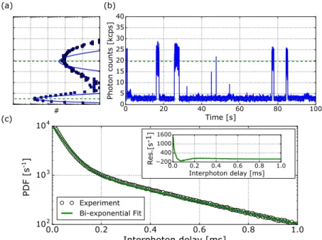
Figure 2 shows the experimental results on our two-intensity system. On panel (a), on the top left, we show the typical histogram of number of photons per bin time, char-acterizing the binned fluorescence time trace of panel (b), which shows the fluorescence time trace. The solid lines in panel (a) are fits with two Poisson distributions. We attribute the deviation from the experimental histogram to additional experimental noise not included in the model. Two levels can be clearly identified. The high-fluorescence level corresponds to hybridized docking and imaging DNA strands so that a dye molecule is immobilized in the hot spot, emitting enhanced flu-orescence. After some seconds, the DNA de-hybridizes either before or after bleaching of the dye, and the imaging strand leaves the hot spot. In both cases, the signal has vanished. The low-level signal corresponds to the luminescence of the gold nanorod itself and to the background fluorescence of dif-fusing and unenhanced molecules in the confocal volume. This system thus fulfills our purpose by providing a stream of detected photons with two well-defined intensity levels.
We would like to retrieve these two levels using the inter-photon delay distribution by fitting a bi-exponential function. Figure2(c)shows the experimental curve and the fitting, from which we extracted the two intensity levels marked in (a) and (b) with dashed lines. These levels clearly reproduce the levels evidenced by the binned time trace and intensity histograms, but they were obtained without the need of any arbitrary bin time.
The results in this simple case show how useful this type of analysis can be, since we were able to extract useful infor-mation from our experimental TTTR data without introducing any arbitrary parameter.
IV. SLOW DIFFUSION IN A 2D GAUSSIAN INTENSITY PROFILE
A more interesting scenario to use our analysis is the prob-lem of two-dimensional diffusion of fluorescent molecules in a Gaussian beam, described by an intensity function
I(r) =I0exp [r2/σ2], where (r,θ) are the normal polar
coor-dinates in the plane andσ represents the waist of the beam. In this case, the intensity profile is bi-dimensional and only
123334-5 Caldarola, Pradhan, and Orrit J. Chem. Phys.148, 123334 (2018)
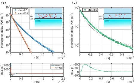
FIG. 3. Bidimensional molecular diffusion probed with a Gaussian beam. (a) Interphoton delay probability density function (PDF) for the case of high con-centrations of molecules, with an average number of moleculeshNi= 7.5 or 120 in the detection areaA=πσ2(corresponding to approximately 14 and 225 molecules/µm2, respectively). The circles are experimental values while the dashed lines are fits with the model from Eq.(10). (b) Interphoton delay probability density function for the case of a low concentration of molecules,hNi= 0.5 (approximately 0.9 molecules/µm2). In this case, we find clear deviations from our model of slow diffusion, possibly indicating averaging of number fluctuations by diffusion, and a more exponential-like decay. The insets show a scheme of the experimental configuration of the lipid bi-layer on the glass surface with the typical dimensions involved (not to scale). In the bottom panel, we show the residuals for the respective fits maintaining the color code.
depends on the distance to the center of the beam. We take a concentrationCof fluorescent molecules per unit area. Using this intensity distribution in Eq.(8), we calculate the expected interphoton delay distribution pG(τ) and find the integral form
pG(τ)=−d
dτ
"
exp −Cσ2π
1
(1
−exp [−τI0u])
du u
!#
,
(10) where ≡exp−σR22 andRis the maximum radius accessi-ble to the diffusing molecules (πR2is the area of the sample).
Because of the smooth variation of the Gaussian beam, many single-molecule bursts have the same maximum intensity. Therefore, FCS provides a good estimate of single-molecule brightness. The case of enhanced fluorescence discussed in Sec.Vis much more difficult to address by FCS.28
We studied the Gaussian case experimentally in a regular confocal microscope by confining the diffusion of ATTO647N dye molecules in a lipid bilayer, obtaining a two-dimensional case and a reduced diffusion coefficient ofD= 4.4 µm2 s1, as presented previously.27
We performed the experiment for high and low con-centrations of molecules in the lipid bilayer and fitted the experimental interphoton curves with pG(τ) from Eq. (10) using the experimental value for the beam waist, σ = 292 nm. Figure 3 shows the experimentally obtained interphoton delay probability density function for high (a) and low (b) concentrations along with the corresponding fits using our theoretical result. We note that the higher the con-centration, the more the delay distribution resembles a sin-gle exponential. Indeed, a sinsin-gle exponential is expected in the limit of extremely high concentrations, where fluctua-tions ∆N of the number of molecules hNi in the Gaussian area become negligible, leading to a constant detected inten-sity and therefore to a single-exponential interphoton delay distribution.
A closer look at the curves in Fig.3reveals that the case of high concentration is well captured with our model while the low-concentration case is not. This is a direct consequence of the main approximation in our model that largely neglects the effect of diffusion. Another phenomenon we have ignored is photobleaching of the molecules in the laser beam. These deviations from our model could thus be studied through the interphoton delay distribution.
V. INTERPHOTON DELAY DISTRIBUTION WITH FLUORESCENCE ENHANCEMENT
We now turn to the case of plasmonic enhancement by an individual nanoparticle. The spatial distribution of fluores-cence enhancement by a plasmonic structure is complex and depends on many parameters. For simplicity’s sake, we model this distribution as a spherically symmetric profile around a spherical nanoparticle. The fluorescence intensity profile is taken as the sum of a Gaussian confocal volume similar to that of Sec.IVand of a near-field component modeled as a steeply decaying power law of radius,
I(r)=W0 "
exp −r 2
σ2
!
+E RNP r
!α#
, r≥RNP, (11)
whereW0 is the unenhanced intensity,σ is the width of the
Gaussian illumination,Eis the maximum enhancement factor at or close to the particle’s surface, andRNPis the nanoparticle
radius. The exponentα is a free parameter used to simulate the short-range variation of the near field. For pure excita-tion enhancement by an electrostatic dipole fieldα = 6, for combined excitation and radiative enhancements of an elec-trostatic dipole field, we would have α = 12. We note that to recover the Gaussian case studied in Sec.IV, we need to takeRNP= 0. In order to obtainp(τ), we insert Eq.(11)into
Eq.(8) and numerically solve the integral forRNP= 25 nm.
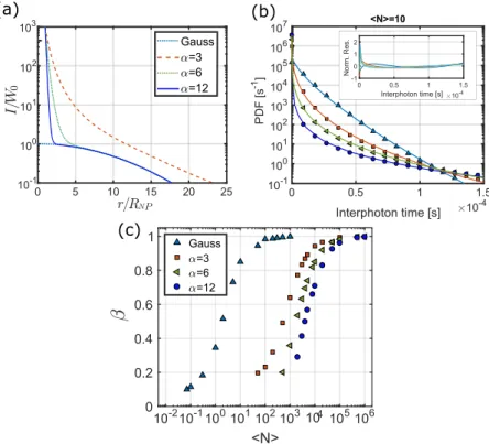
FIG. 4. Simple model for plasmonic enhancement in two dimensions. (a) Normalized radial intensity distributions for Gaussian (blue dotted line) and near field model with
α= 3 (red dashed line),α= 6 (green dotted line), andα = 12 (blue solid line). For all the cases, the unenhanced intensity isW0= 1.5×10⁴cps and for the enhanced case we usedRNP= 25 nm andE= 1000. (b) Interphoton delay probability density function for the three cases pre-sented in (a) for a mean number of moleculeshNi= 10 in the Gaussian area. The symbols present the data from the numerical evaluation ofp(τ) and the solid lines are fits with stretched exponentials. We intentionally reduced the density of points for display. The inset shows the nor-malized residuals from the fits. (c) Extractedβfrom the stretched exponential fit as a function of the mean num-ber of molecules in the Gaussian area. The color code is maintained throughout the whole figure.
explore the effect of the near field. It completely ignores quenching, polarization, and the complex spatial structure of the near field.
Figure 4(a) shows the comparison of the spatial inten-sity distribution for three different values of the exponentα with the unenhanced case. With these intensity spatial distri-butions, we calculated the interphoton delay distribution by numerically solving the integral in Eq.(8). Note that the area inside the nanoparticle is not accessible to the molecules so the integration was carried forr≥RNP. The obtained
distribu-tions are shown in Fig.4(b)for the case ofhNi= 10 molecules in the Gaussian area (A=πσ2). Clearly the distributions with enhancement show more probability density at extremely short interphoton times, corresponding to the high emission rates produced by molecules occasionally entering the near-field area with high enhanced intensities. These events correspond to bright bursts in the fluorescence time trace. The lower the concentration of molecules, the more seldom these events will be, and the further away the delay distribution will be from a single exponential.
In order to qualitatively compare the interphoton delay distributions for the different cases, we decided to fit them with stretched exponentials
f(τ)=Aexpf−(λτ)βg (12)
to characterize the deviation of the interphoton delay distri-bution from a single exponential. As we mentioned before, in the case of very high molecular concentrations we expect to recover β= 1, i.e., an exponential behavior, whereas large number fluctuations will give rise to strong deviations from single exponential and to a smaller stretching exponent. The empiric fit function in Eq. (12) works reasonably well for short times, but fails to reproduce the long-time tails of the delay distribution. Therefore, we focus our analysis on the
short-time domain, which contains the most useful information about plasmonic enhancement.
We fitted the calculated probability density functions for different concentrations of molecules ranging from a very diluted sample (1 molecule in the Gaussian area, 3×10³ in the near-field area) to an extremely high number of molecules (106in the Gaussian area, 3×10³in the near field). Figure4(c)
shows the obtained stretching exponent β as a function of concentration and for the Gaussian beam and the enhanced case with three different exponents α= 3, 6, and 12. In the Gaussian case, we obtain an exponential behavior, charac-terized with β= 1 only forhNi ≥ 100. This corresponds to the situation when number fluctuations in the detection area are negligible and thus a nearly constant detected intensity is obtained.
To obtain a single-exponential interphoton delay distribu-tion in the enhanced case, we should reach the high-density regime mentioned above, but considering the near-field area. Since the ratio of the near-field areaANF [considered as the
area that contains intensities higher thanEW0exp (1)] and
the far-field areaAFF =πσ2 is ANF
AFF ∼3×10
−3, we roughly
expect a difference of 3 orders of magnitude in the number of molecules needed to reach the single-exponential limit. Indeed, this is what our curves show, where for the enhanced case we approach β= 1 aroundhNi= 105.
123334-7 Caldarola, Pradhan, and Orrit J. Chem. Phys.148, 123334 (2018)
VI. FLUORESCENCE TIME TRACES
WITH ENHANCEMENT BY A GOLD NANOROD
We now turn to results of an experiment with configu-ration similar to the one presented in Sec. IV. A Gaussian beam is focused on a single gold nanorod immobilized on a glass substrate, and dye molecules diffuse in a lipid bi-layer deposited on the same substrate, similar to Ref.27. A fluores-cence signal is produced whenever a dye molecule enters the diffraction-limited Gaussian beam, and an enhanced fluores-cence signal appears if the molecule then enters either of the plasmonic hot spots around the tips of the gold nanorod. In order to obtain the enhancement value, we need to compare the detected intensity from a single-molecule enhancement event with the unenhanced intensity detected using the same experimental conditions, which was 100 kcps.27
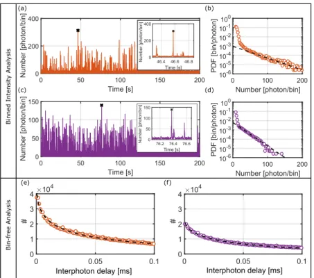
Figure5presents the TTTR experimental data obtained in such an experiment in different ways, for two different gold nanorods. In the top panel, we have the bin-dependent time traces and burst histograms (binning time 1 ms) while the lower panel shows the “bin-free” interphoton delay histograms. If we analyze the binned time traces in Figs.5(a)and5(c)and the insets, we observe that they present a qualitatively simi-lar behavior: there is a constant baseline intensity, long weak bursts corresponding to molecules exploring the far field area and occasionally intense but short bursts corresponding to dif-fusion in the near-field area.27The black crosses in the time traces indicate the highest burst found in that trace, which leads to “cherry picking” enhancements factorsE(CP)= (4.5±1.5) andE(CP)= (2.3±0.7).
Another useful way to characterize the experimental enhancement is the histogram of binned intensities, as shown in Figs.5(b)and5(d). These histograms show a rapidly decay-ing tail where the characteristic decay intensity is larger for the top nanorod, indicating stronger enhancement. The steep
decay of these histograms can be qualitatively understood by recalling the spatial distribution of near-field intensity at reso-nance, which is extremely high (around 300 times the incident intensity) very close to the tips and decays rapidly with dis-tance to the tips. Therefore, there is a low probability for a diffusing molecule to reach this small area. For small dis-tances, this probability density goes linearly with distance in the bi-dimensional case and as the squared distance in the three-dimensional case.
We analyzed the intensity distribution around a rod (25
×47 nm2), calculated from a discrete-dipole approximation.9 In the 2D case, we found an approximate power law distribu-tion with exponent 1.37. However, the tail of the experimental distribution is exponential, as can be seen in Figs. 5(b)and
5(d). There are several possible sources for such a discrep-ancy, such as the effect of photobleaching, the dead time of the detectors, and possibly the role of diffusion during the burst. Confirming the role of each of these effects would require full numerical calculations, with an accurate descrip-tion of these effects. However, this is a complex and compu-tationally extensive problem that is out of the scope of this paper.
Regardless of the reason for this deviation, we may empir-ically estimate the maximum enhancement through the his-togram. Note that stronger enhancement corresponds to a broader histogram, with cutoff for larger photon number. If we model the tail of the normalized histogram decay as a single exponential P(N) =Mexp (N/N0), we can estimate
the maximum number of photons in the strongest burst by solvingP(Nc) =ε withε = 1/Nbins, whereNbins is the total
number of bins in the time trace, here about 106. This esti-mate roughly corresponds to a probability equal to unity of observing such an intense burst in the time trace. We thus obtainNc=N0ln (M/ε). For a typical value ofM ∼×103,
we find 6.9N0. With this method we obtainE(H)= (4.9±0.2)
andE(H) = (2.40 ±0.05) for the plotted data in Figs. 5(b)
and5(d).
Enhancement factors could also be extracted from an FCS analysis.27,28,35 However, this technique is very sensitive to background corrections and the relation between enhancement factor and correlation contrast is model-dependent.
We can also estimate the enhancement factor from the interphoton delay histograms. These histograms are shown for the same two nanorods in Figs.5(e)and5(f). Deviations from single-exponentials are clearly seen. To characterize them, we fit the histograms with a stretched exponential of time [see Eq.(12)], which involves only three parameters, against four for a bi-exponential decay. The maximum enhanced inten-sity is deduced from the slope of the histogram at the shorter measured interphoton time (200 ns) and provides another esti-mate of the enhancement factor based on a statistical quantity. Figures 5(e)and5(f) show that larger enhancements corre-spond to a larger deviation of the histogram from a single exponential and to a larger slope at the smallest bin time of the histogram. With this procedure, we obtained an enhance-ment value ofE(I)= (4.3±0.2) andE(I)= (2.0±0.1) for the
presented nanorods.
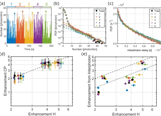
We now compare the maximum intensities and the associ-ated enhancement factors obtained for five different nanorods, for the whole 200 s-long time trace, and after splitting each trace into 5 sub-traces of 40 s each. Figure6shows the exam-ple of the binned time trace (a), burst histogram (b), and the
interphoton delay histogram (c) for the whole trace and for each sub-trace.
The associated results for the different methods are cor-related in Figs. 6(c) and 6(d). The different symbols cor-respond to different nanorods and the colors refer to the different sub-traces for each rod. In Fig. 6(d), we observe an excellent correlation between the cherry-picking method and the statistical method based on the burst intensity his-tograms. Note that the same symbols are clustered together, showing that the enhancement factor obtained using differ-ent sub-traces with both methods lead to similar results. We also correlated the results from the interphoton delay dis-tribution with the burst intensity histograms in Fig. 6(e), where a satisfactory correlation is found and the obtained enhancement factors are consistent with both other methods. However, the enhancement factors deduced from interpho-ton delay distributions present more dispersion than the other two.
Figure6confirms that the estimates of the enhancement factor deduced by three very different methods (time trace, burst histogram, and interphoton delays) are similar in value and consistent with one another. The values deduced from the cherry-picking procedure are surprisingly stable and reli-able. They agree well with extrapolations of burst histograms fitted with a single-exponential function, although the justifica-tion for this analytical form is still missing. Unexpectedly, the enhancement factor deduced from the interphoton histogram
123334-9 Caldarola, Pradhan, and Orrit J. Chem. Phys.148, 123334 (2018)
appears to be the most sensitive to statistical fluctuations. This can be a consequence of fitting with a stretched exponen-tial, which is an approximation. However, this method has the unique advantage that it can be applied to the experimental data directly, without any need for binning or other arbitrary parameters.
VII. CONCLUSIONS
In this paper, we characterized single-molecule fluores-cence traces obtained with a time-tagged time-resolved setup in a variety of experimental conditions with the interphoton delay distribution. This avoids the introduction of an arbitrary binning time.
We presented a theoretical treatment for the case of nearly static, slowly diffusing molecules that relates the interphoton delay distribution to the spatial intensity distribution explored by the molecules. With this model, we could reproduce the simple case of switching between two states with different intensities. We also explored the problem of molecules dif-fusing in two dimensions in a Gaussian beam. Our nearly static model works well at high concentrations, but shows deviations at lower concentrations, which may arise from diffusion or from other experimental deviations from the model.
Furthermore, we used the interphoton delay distribution to measure the fluorescence enhancement factor by individ-ual gold nanorods. For our experimental traces with moderate enhancements, we obtained enhancement factors that are con-sistent with the accepted methods in the community with the advantage of avoiding the introduction of any arbitrary param-eter that may influence the results. In the future, we plan to perform similar comparisons for the very large enhancement factors obtained with weakly emitting dyes.
ACKNOWLEDGMENTS
We would like to acknowledge financial support from NWO, the Netherlands Organization for Scientific Research, Grant No. ECHO 712.013.003 and the NanoFront program.
1W. Moerner and M. Orrit, “Illuminating single molecules in condensed matter,”Science283(5408), 1670–1676 (1999).
2F. Kulzer, T. Xia, and M. Orrit, “Single molecules as optical nanoprobes for soft and complex matter,”Angew. Chem., Int. Ed.49(5), 854–866 (2010).
3W. Zhang, M. Caldarola, B. Pradhan, and M. Orrit, “Gold nanorod enhanced fluorescence enables single-molecule electrochemistry of methylene blue,”Angew. Chem., Int. Ed.56(13), 3566–3569 (2017).
4E. A. Jares-Erijman and T. M. Jovin, “Fret imaging,”Nat. Biotechnol. 21(11), 1387–1395 (2003).
5I. H. Stein, V. Sch¨uller, P. B¨ohm, P. Tinnefeld, and T. Liedl, “Single-molecule FRET ruler based on rigid DNA origami blocks,”ChemPhysChem12(3), 689–695 (2011).
6S. Kalinin, T. Peulen, S. Sindbert, P. J. Rothwell, S. Berger, T. Restle, R. S. Goody, H. Gohlke, and C. A. Seidel, “A toolkit and benchmark study for FRET-restrained high-precision structural modeling,” Nat. Methods
9(12), 1218–1225 (2012).
7A. Kinkhabwala, Z. Yu, S. Fan, Y. Avlasevich, K. M¨ullen, and W. Moerner, “Large single-molecule fluorescence enhancements produced by a bowtie nanoantenna,”Nat. Photonics3(11), 654–657 (2009).
8H. Yuan, S. Khatua, P. Zijlstra, M. Yorulmaz, and M. Orrit, “Thousand-fold enhancement of single-molecule fluorescence near a single gold nanorod,”
Angew. Chem., Int. Ed.52(4), 1217–1221 (2013).
9S. Khatua, P. M. Paulo, H. Yuan, A. Gupta, P. Zijlstra, and M. Orrit, “Reso-nant plasmonic enhancement of single-molecule fluorescence by individual gold nanorods,”ACS Nano8(5), 4440–4449 (2014).
10T. S. van Zanten, M. J. Lopez-Bosque, and M. F. Garcia-Parajo, “Imaging individual proteins and nanodomains on intact cell membranes with a probe-based optical antenna,”Small6(2), 270–275 (2010).
11L. C. Estrada, P. F. Aramend´ıa, and O. E. Mart´ınez, “10 000 times volume reduction for fluorescence correlation spectroscopy using nano-antennas,”
Opt. Express16(25), 20597–20602 (2008).
12C. Manzo, T. S. van Zanten, and M. F. Garcia-Parajo, “Nanoscale fluores-cence correlation spectroscopy on intact living cell membranes with NSOM probes,”Biophys. J.100(2), L8–L10 (2011).
13A. A. Kinkhabwala, Z. Yu, S. Fan, and W. Moerner, “Fluorescence correla-tion spectroscopy at high concentracorrela-tions using gold bowtie nanoantennas,”
Chem. Phys.406, 3–8 (2012).
14D. Punj, J. de Torres, H. Rigneault, and J. Wenger, “Gold nanoparti-cles for enhanced single molecule fluorescence analysis at micromolar concentration,”Opt. Express21(22), 27338–27343 (2013).
15S. Khatua, H. Yuan, and M. Orrit, “Enhanced-fluorescence correlation spec-troscopy at micro-molar dye concentration around a single gold nanorod,”
Phys. Chem. Chem. Phys.17(33), 21127–21132 (2015).
16V. Flauraud, T. S. van Zanten, M. Mivelle, C. Manzo, M. F. Parajo, and J. Brugger, “Large-scale arrays of bowtie nanoaperture antennas for nanoscale dynamics in living cell membranes,” Nano Lett. 15(6), 4176–4182 (2015).
17M. Wahl,Time-Correlated Single Photon Counting, Technical report, (Pico-Quant, Berlin, Germany, 2014); see http://www.picoquant.com/images/ uploads/page/files/7253/technote tcspc.pdf.
18W. Becker,Advanced Time-Correlated Single Photon Counting
Applica-tions, Springer Series in Chemical Physics (Springer, 2015), Vol. 111. 19The usual denomination is microtime but we opt for nanotime to avoid
confusion with the macrotime.
20J. Lakowicz, Principles of Fluorescence Spectroscopy (Springer US, 2007).
21M. Lippitz, F. Kulzer, and M. Orrit, “Statistical evaluation of single nano-object fluorescence,”ChemPhysChem6(5), 770–789 (2005).
22D. Magde, E. Elson, and W. W. Webb, “Thermodynamic fluctuations in a reacting system—Measurement by fluorescence correlation spectroscopy,”
Phys. Rev. Lett.29(11), 705 (1972).
23E. Haustein and P. Schwille, “Fluorescence correlation spectroscopy: Novel variations of an established technique,”Annu. Rev. Biophys. Biomol. Struct.
36, 151–169 (2007).
24A. Loman, I. Gregor, C. Stutz, M. Mund, and J. Enderlein, “Measur-ing rotational diffusion of macromolecules by fluorescence correlation spectroscopy,”Photochem. Photobiol. Sci.9(5), 627–636 (2010). 25M. A. Medina and P. Schwille, “Fluorescence correlation spectroscopy for
the detection and study of single molecules in biology,”BioEssays24(8), 758–764 (2002).
26A. Ghosh, S. Isbaner, M. Veiga-Guti´errez, I. Gregor, J. Enderlein, and N. Karedla, “Quantifying microsecond transition times using fluorescence lifetime correlation spectroscopy,”J. Phys. Chem. Lett.8(24), 6022–6028 (2017).
27B. Pradhan, S. Khatua, A. Gupta, T. Aartsma, G. Canters, and M. Orrit, “Gold-nanorod-enhanced fluorescence correlation spectroscopy of fluo-rophores with high quantum yield in lipid bilayers,”J. Phys. Chem. C120, 25996–26003 (2016).
28L. Langguth and A. F. Koenderink, “Simple model for plasmon enhanced fluorescence correlation spectroscopy,”Opt. Express22(13), 15397–15409 (2014).
29R. Verberk and M. Orrit, “Photon statistics in the fluorescence of single molecules and nanocrystals: Correlation functions versus distributions of on- and off-times,”J. Chem. Phys.119(4), 2214 (2003).
30Note that the Laplace transformation is usually applied to time-dependent functions, giving rate-dependent functions. Here, we apply it to a function of the rate and thus obtain a time-dependent transform.
31A. M. Stoneham, “Shapes of inhomogeneously broadened resonance lines in solids,”Rev. Mod. Phys.41, 82–108 (1969).
33G. Acuna, F. M¨oller, P. Holzmeister, S. Beater, B. Lalkens, and P. Tinnefeld, “Fluorescence enhancement at docking sites of DNA-directed self-assembled nanoantennas,” Science 338(6106), 506–510 (2012).
34R. Jungmann, C. Steinhauer, M. Scheible, A. Kuzyk, P. Tinnefeld, and F. C. Simmel, “Single-molecule kinetics and super-resolution microscopy
by fluorescence imaging of transient binding on DNA origami,”Nano Lett.
10(11), 4756–4761 (2010).