Design considerations for complex survival models

(1)

DESIGN CONSIDERATIONS FOR COMPLEX

SURVIVAL MODELS

Liddy Miaoli Chen

A dissertation submitted to the faculty of the University of North Carolina at Chapel Hill in partial fulﬁllment of the requirements for the degree of Doctor of Philosophy in the Department of Biostatistics, Gillings School of Global Public Health.

Chapel Hill 2010

Approved by:

(2)

c

2010

(3)

ABSTRACT

LIDDY MIAOLI CHEN: DESIGN CONSIDERATIONS FOR COMPLEX SURVIVAL MODELS.

(Under the direction of Dr. Joseph G. Ibrahim and Dr. Haitao Chu.)

Various complex survival models, such as joint models of survival and longitudinal

data and multivariate frailty models, have gained popularity in recent years because

these models can maximize the utilization of information collected. It has been shown

that these methods can reduce bias and/or improve eﬃciency, and thus can increase

the power for statistical inference. Statistical design, such as sample size and power

calculations, is a crucial ﬁrst step in clinical trials.

We derived a closed form sample size formula for estimating the eﬀect of the

longitu-dinal process in joint modeling, and extend Schoenfeld’s (1983) sample size formula to

the joint modeling setting for estimating the overall treatment eﬀect. The sample size

formula we developed is general, allowing for p-degree polynomial trajectories. The

ro-bustness of our model was demonstrated in simulation studies with linear and quadratic

trajectories. We discussed the impact of the within subject variability on power, and

data collection strategies, such as spacing and frequency of repeated measurements, in

order to maximize power. When the within subject variability is large, diﬀerent data

collection strategies can inﬂuence the power of the study in a signiﬁcant way.

We also developed a sample size determination method for the shared frailty model

to investigate the treatment eﬀect on multivariate time to events, including recurrent

events. We ﬁrst assumed a common treatment eﬀect on multiple event times, and the

sample size determination was based on testing the common treatment eﬀect. We then

(4)

time-to-events as nuisance, and compared the power from a multivariate frailty model

versus that from a univariate parametric and semi-parametric survival model. The

multivariate frailty model has signiﬁcant advantage over the univariate survival model

when the time-to-event data is highly correlated.

Group sequential methods had been developed to control the overall type I error rate

in interim analysis of accumulating data in a clinical trial. These methods mainly apply

to testing the same hypothesis at diﬀerent interim analyses. Finally, we extended the

methodology of the alpha spending function to group sequential stopping boundaries

when the hypotheses can be diﬀerent between analyses. We found that these stopping

boundaries depend on the Fisher’s Information matrix, and application to a bivariate

(5)

ACKNOWLEDGMENTS

I would like to thank my advisor, Dr. Joseph Ibrahim, and my co-advisor, Dr. Haitao

Chu, for their encouragement, mentorship, and research ideas during the preparation

and completion of this dissertation. Special thanks goes to Dr. Ibrahim who kept

pushing me when I was slow and felt I had nowhere to go. During my long journey

of graduate studies at UNC Chapel Hill, I had received numerous help from diﬀerent

faculty members, and I would speciﬁcally like to thank Dr. Joseph Ibrahim again

and Dr. Donglin Zeng for their help during the summer of 2007 when I prepared my

qualifying exam. I could not have come to this point without making that important

step. I would also like to thank my other committee members (Dr. William Irvin Jr.,

Dr. Donglin Zeng, and Dr. Hongtu Zhu) for their time to review my papers and their

comments.

My deepest appreciation goes to my family, especially my mother, who had given me

endless support and encouragement. Most importantly, I need to thank my daughter,

Vanessa Lin, for the sacriﬁce she made. There are countless times that mom could not

play with her because mom had to “work”. It is to her that I would like to dedicate

(6)

LIST OF TABLES

2.1 Validation of formula (2.4) for testing the trajectory eﬀect_β when Σθ is

known . . . 20

2.2 Power for estimating _β by maximum number of data collection points (_mx) and size of σ2e - linear trajectory . . . 25

2.3 Power for estimating _β by maximum number of data collection points (_mx) and size of σ2e - quadratic trajectory . . . 26

2.4 Validation of formula (2.12) for testing the overall treatment effect_α+_βγ 30 2.5 Effect of _β on the estimation of direct treatment effect on survival (_α)

based on diﬀerent models . . . 31

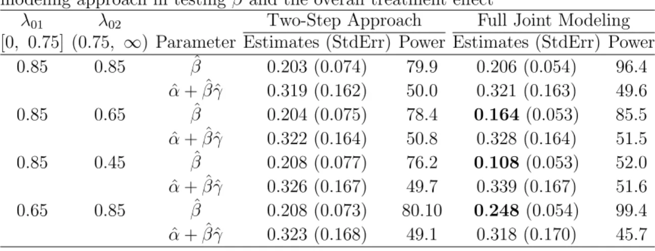
2.6 Comparison of the two-step inferential approach with the full joint mod-eling approach in testing_β and the overall treatment eﬀect . . . 32 2.7 Parameter Estimates with Standard Errors for the E1193 Data . . . 40

3.1 Comparison of Empirical Power and Calculated Power for Testing a Common Treatment Eﬀect with Diﬀerent Model Parameters . . . 49

3.2 Estimating and Testing _β₁ in Multivariate Time-to-Events with _K = 3 and _eβ0 _{= 0}_._{05 Using Different Models} _{. . . .} ₅₃ 3.3 Estimating and Testing_β₁ Using Different Models by Different Baseline

Event Rates . . . 54

3.4 Estimating and Testing_β₁: Empirical and Calculated Power by Diﬀerent Correlation Between Event Times (_K = 3, _γ = 2, _eβ₀ _{= 0}_._{05, and}

eβ1 _{= 0}_._{8) . . . .} ₅₆ 4.1 One-sided Boundaries for Diﬀerent Values of _w with _α = 0_.025 and

K = 5 (The test parameter is assumed to be _θ₁ for _j = 1_,2, _θ₂ for j = 3_,4_,5, where _j = 1_{, . . . ,}5,_t∗_j =_j/5.) . . . 70 4.2 One-sided Boundaries for the 5th Analysis _zc(5) When α = 0.025 and

K = 5 (The test parameter is assumed to be _θ₁ for _j = 1−4, _θ₂ for j = 5, where _j = 1_{, . . . ,}5,_t∗_j =_j/5.) . . . 71 4.3 One-sided Boundaries for Diﬀerent Values of _w with _α = 0_.025, _K = 2

(10)

(11)

CHAPTER 1 Introduction and Literature Review

1.1 Introduction

Various complex survival models, such as joint models of survival and longitudinal data

and multivariate frailty models, have gained popularity in recent years because these

models can maximize the utilization of information collected. Classical models such as

the Cox proportional hazard model to handle time-to-event data and the mix model

to handle repeated measurements evaluate the treatment eﬀect on these two types of

responses separately. There are two complications in describing or making inference

on the longitudinal process in these studies: 1) Occurrence of the time-to-event may

induce an informative censoring (Wu and Carroll 1988, Hogan and Laird 1997ab), as

subjects who have early events would be censored at an earlier time point. 2) The

longitudinal data is only available intermittently for each subject, and likely subjects

to measurement errors. These concerns led to the development of joint models of the

two data types. Joint models are also developed because there is a need to take into

account the dependency of these two data types when investigating the treatment eﬀect

on survival.

The need to study or analyze multiple correlated time-to-event data arises in many

(12)

increasingly popular for analyzing multivariate time-to-event data (Oakes 1989,

Peter-son 1998, Duchateau et al. 2003, Cook and Lawless 2007, Zeng et al. 2009) because it

provides a convenient way to introduce association and unobserved heterogeneity into

models for the multivariate survival data. A frailty, a concept introduced by Vaupel et

al. (1979), is an unobservable random eﬀect. A natural way to model dependence of

clustered or multivariate event times is through the introduction of a cluster-speciﬁc

random eﬀect. This random eﬀect explains the dependence in the sense that had we

known the frailty, the events would be independent.

Design is a crucial ﬁrst step in clinical trials. Well-designed studies are essential

for successful research and drug development. Although much eﬀort has been put into

inferential and estimation methods in these complex survival models, design researches

are lacking. Sample size determination for these models have not been formally

consid-ered. There has been little guidance in the methodologic literature as to how researchers

should select the number of repeated measures for the longitudinal data. Hence

devel-oping statistical methods to address design issues in joint modeling and multivariate

frailty model are much needed.

Interim analyses are also commonly used in clinical trials due to diﬃculty in

enroll-ment, and/or long follow-up time until enough events have occurred. Although much

ﬂexibility has been achieved with the alpha spending function in group sequential

de-signs, the unique feature of joint model also brings up another group sequential design

model. In Chapter 2, a sample size formula to study the association between the

time-to-event and the longitudinal data is provided, followed by detailed discussion of the

methodology when the variance-covariance matrix is known or unknown. Longitudinal

data collection strategies, such as spacing and frequency of repeated measurements, to

maximize the power are also discussed. Chapter 3 provides a sample size determination

formula to study a common treatment eﬀect for the multivariate time-to-event data,

(13)

while taking into account the dependency of clustered event times. Group sequential

design when diﬀerent parameters are involved is discussed is discussed in Chapter 4,

followed by application in multivariate survival models and joint models.

1.2 Joint Models in the Literature

1.2.1 Two-Step Models

The earliest literature on joint modeling focuses on a two-step inferential strategy which

deﬁnes sub-models for the longitudinal and event time processes (Self and Pawitan 1992,

Tsiatis and Wulfsohn 1995). In “ideal” data situation, the longitudinal process follows

a well-deﬁned trajectory, {_Xi(u), u ≥ 0)}, for all times u ≥ 0 for each subject i =

1_{, . . . , n}. A routine framework to study the association between the time-to-event and the treatment eﬀect, or the association between the time-to-event and the longitudinal

data, is to represent the relationship between the event time (_Ti), the trajectory (Xi(u)),

and the baseline covariates (Zi) by a proportional hazard model (Cox 1975)

λi(u) = lim du→0du

−1_pr_u_≤_t

i < u+du|ti ≥u, XiH(u),Zi

= _λ₀(_u)exp_βXi(u) +αTZi

, (1.1)

where_XH

i (u) ={Xi(t),0≤t < u}is the history of the longitudinal process up to time

u. Inference on _β and _α can be made by maximizing the partial likelihood.

n

i=1

exp{_βXi(Si) +αTZi}

n

k=1exp{βXk(Si) +αTZk}I(Sk≥Si)

Δi

, (1.2)

where _S_i = min(_T_i_{, C}_i) (_T_i and _C_i denote the event and censoring times, respectively) and Δi = I(Ti ≤ Ci). However, Xi(u) is unknown, and the response is collected on

(14)

value of

fX(_u)_{, β, α} = exp{_βX(_u) +_αTZ}

is given by

Eexp{_βX(_u) +_αTZ|_Y¯(_u)_{, u < S}}_, (1.3) where ¯_Y(_u) is the history of observed longitudinal data up to time u. Theoretical justiﬁcation for this two-stage model is that the value of (1.3) can be approximated by

a ﬁrst-order approximation:

Eexp{_βX(_u) +_αTZ|_Y¯(_u)_{, u < S}}

≈ exp{_βE_X(_u)|_Y¯(_u)_{, u < S}+_αTZ}_.

Therefore, we can replace the unknown value, _Xi(Si) in (1.2) withE

Xi(Si)|Y¯i(Si)

.

Let _Yi(tij) = Xi(tij) +ei(tij) denote the observed value of Xi(tij), where ei(tij) is an

intra-subject error and is normally distributed with mean 0. Tsiatis and Wulfsohn

(1995) proposed a simple linear model

Xi(u) = θ0i+θ1iu (1.4)

to represent the log CD4 trajectories. A more general polynomial model _Xi(u) =θ0i+

θ1iu+θ2iu2+· · ·+θpiup had been considered in later studies (Chen et al. 2004, Ibrahim

et al. 2004). In this model, it is assumed that each subject followed his or her own

trajectory with intercept _θ₀i and slope θ1i. (θ0i, θ1i)T are i.i.d bivariate normal vectors

with mean (_μ₀_{, μ}₁)T _{and variance-covariance} _Σ

θ. Consequently, E

Xi(Si)|Y¯i(Si)

can

be represented by ˆ_θ₀i and ˆθ1i, the Bayes estimates of θ0i and θ1i. One way to obtain

(15)

and Ware (1982).

1.2.2 The Likelihood Approach

Several drawbacks to the two-step modeling were discussed by Wulfsohn and Tsiatis

(1997), and Tsiatis and Davidian (2004). The most important drawback is that the

random eﬀects in those at risk at each event time is probably not normally distributed,

a critical assumption for the mixed model. If the longitudinal data is predictive of

survival, patients with the steepest slope will be removed from the at risk population

at an earlier time point. Thus it is less likely that the normality assumption still holds as

time progresses. Other drawbacks include the validity of the ﬁrst order approximation

and less eﬃcient use of information.

Wulfshon and Tsiatis (1997) proposed a full data likelihood incorporating a linear

model for the longitudinal data and the Cox model for the time-to-event data as

_∞

−∞ m_j

j=1

f(_Yij|θi, σ2e)

f(_θi|μθ,Σθ)f(Si,Δi|θi, β)dθi. (1.5)

In expression (1.5), _f(_Yij|θi, σ2e) is a univariate normal density function with mean

θ0i+θ1itij and variance σe2, and f(θi|μθ,Σθ) is the multivariate normal density with

mean_μθ and covariance matrix Σθ. The density function for the time-to-event is based

on Cox partial likelihood, where

f(_Si,Δi|θi, β, α) = {λ0(Si) exp[β(θ0i+θ1iSi)]}Δi

× exp

−

S_i

0

λ0(t) exp[β(θ0i+θ1it]dt

.

The parameters_θ,Σθ,σe2, andβ were estimated using parametric maximum likelihood,

(16)

similar to those from the two-step model (the same data was used), with ˆ_βfurther from the null as compared to that from the two-step model.

Alternative forms to model the “true” longitudinal process has been considered

(Song et al. 2002b, Taylor et al. 1994, Lavalley & DeGruttola 1996, Wang & Taylor

2001, Henderson et al. 2000, and Xu & Zeger 2001)

1.3 Multivariate Frailty Models in the Literature

The shared frailty model, ﬁrst introduced by Clayton (1978), assumes that individuals

in a cluster or repeated measurements of an individual share the same frailty,_ω, and the survival times are assumed to be conditional independent with respect to the shared

(common) frailty. Conditional on the frailty, the hazard function of an event in an

individual, or an individual in a cluster is of the form _ωλ₀(_t)exp(_βTX), where _ω is common to all events in an individual. The survival function is given as

S(_t₁_{, . . . , t}K|ω) =S1(t1)ωS2(t2)ω. . . SK(tK)ω.

Independence of the survival times within an individual corresponds to a degenerate

frailty distribution with variance equals 0. One major consideration in the frailty

mod-els is the choice of the frailty distribution. Clayton (1978) and Oakes (1982) ﬁrst

considered frailty models with gamma distribution for the frailty. In a gamma frailty

model, the frailty can be easily integrated out and thus the data likelihood has a closed

form. This is also the model considered in this paper. Hougaard discussed

multivari-ate failure models, where the frailty follows a positive stable distribution (Hougaard

1986a) or a power variance family (PVF) distribution (Hougaard 1986b). Whitmore

and Lee (1991) proposed a model with inverse Gaussian frailty and constant hazard.

(17)

Lognormal frailty model (McGilchrist and Aisbett 1991, Korsgaard et al. 1998) has

gained popularity recently especially in Bayesian models. The selection of the family

of frailty distributions, based on the properties of the various models was discussed by

Hougaard (1995).

Besides the shared frailty model, other frailty models have been considered to handle

more complex multivariate time-to-event data. The correlated frailty model (Pickles

et al. 1994, Yashin & Iachine 1995, Wienke et al. 2001) is not constrained to have a

common frailty. The frailty for each event time is associated by a joint distribution

instead. Price and Manatunga (2001) considered the use of cure frailty models to

analyze a leukaemia recurrence with a cured fraction. The nested frailty model that

accounts for the hierarchical clustering of the data by including two nested random

eﬀects is considered by Rondeau et al. (2006). Most recently, joint frailty models for

modeling recurring events and death has been proposed (Rondeau et al. 2007).

1.4 Group Sequential Methods and Alpha

Spend-ing Functions in the Literature

It is fundamental to have a trial that is properly designed to answer the scientiﬁc

question, such as whether the drug improves overall survival, and every trial design

is striving to answer the question with most robustness and accuracy while involving

the least number of patients and the shortest duration of time. Theories for group

sequential clinical trials has developed largely during the past few decades so that

a trial can be stopped early if there is strong evidence of eﬃcacy during any planned

interim analysis. A high degree of ﬂexibility has been established with respect to timing

of the analyses and how much type I error (alpha) to spend at each analyses. Popular

methods include the Pocock group sequential boundaries (Pocock 1977), the

(18)

ﬁrst introduced by Lan and DeMets (1983).

1.4.1 Group Sequential Boundaries

Let_Z(_k) denote the test statistic using the cumulative data up to analysis_k, and_Z∗(_k) denote the test statistic using data accumulated between the (_k−1)th analysis the_kth analysis, then

Z(_k) ={_Z∗(1) +· · ·+_Z∗(_k)}_/√_k.

The distribution of _Z(_k)√_k can be written as a recursive density function evalu-able by numerical integration (Armitage et al. 1969). The probability of crossing the

boundary for the very ﬁrst time at each interim analysis can be calculated based on

this density function. Under _H₀, the sum of these probabilities should equal to the nominal overall type I error rate for the group sequential design.

Pocock (1977) ﬁrst proposed that the crossing boundary be constant for all equally

spaced analyses, with _zc(k) = zc for all k = 1,2. . . , K. O’Brien and Fleming (1979)

suggested that_zc(k) be changed over theK analyses such that zc(k) =zOBF

K/k. In both procedures, the number of interim analyses and the timing of the interim analyses

need to be pre-determined. The O’Brien-Fleming boundaries have been used more

frequently because it still preserves a nominal signiﬁcance level at the ﬁnal analysis

that is close to that of a single test procedure. An earlier work by Haybittle and

Peto (Haybittle 1971, Peto et al. 1976) in a less formal structure suggested to use

an arbitrarily large value for the crossing boundary for each interim analysis, and the

boundary for the ﬁnal analysis should be determined such that the overall type I error

(19)

1.4.2 The Alpha Spending Function

The alpha spending function initially developed by Lan and DeMets (1983) over the

course of a group sequential clinical trial is a more ﬂexible group sequential procedure

that does not require the total number nor the exact time of the interim analyses to be

speciﬁed in advance.

Speciﬁcally, let _T denote the scheduled end of the trial, and _t∗ denote the fraction of information that has been observed at calendar time _t (_t ∈ [0_{, T}]. Also let _ik, k =

1_,2_{, . . . , K} denote the information available at the kth interim analysis at calendar time tk, so t∗k =ik/I, where I is the total information. Lan and DeMets speciﬁed an alpha

spending function such that _α(0) = 0 and _α(1) = _α. Boundary values _zc(k) can be

determined successively so that

P0{|Z(1)| ≥zc(1), or|Z(2)| ≥zc(2), or . . . , or|Z(k)| ≥zc(k)}=α(t∗k) (1.6)

where {_Z(1)_{, . . . , Z}(_k)} are the test statistics from the interim analyses 1_{, . . . , k}. Alpha spending functions that approximate O’Brien-Fleming or Pocock Boundaries

are as follows:

O’Brien-Fleming: _α₁(_t∗) = 2−2Φ(_Zα/2/

√

t∗) Pocock: _α₂(_t∗) = _αIn(1 + (_e−1)_t∗)

where Φ denotes the standard normal cumulative distribution function. The other

alpha spending function proposed in the paper is _α₃(_t∗) = _αt∗, representing uniform spending of alpha over time. _α₃(_t∗) is intermediate between functions_α₁(_t∗) and_α₂(_t∗). To solve for the boundary values_zc(k), we need to obtain the multivariate distribution

(20)

parameter at each interim analysis.

σlk = cov{Z(l), Z(k)}

=

t∗l/t∗k =

il/ik

= _nl/nk, l≤k,

where_nl and nk are the number of subjects included in thelth and kth interim

analy-ses. If the information increments have independent distributional structure, which is

usually the case, derivation of _zc(k) based on α(t∗) is relatively straightforward with

this covariance structure using the methods of Armitage et al. (1969).

Earlier development of the alpha spending function was based on assumption that

information accumulated between each interim analysis is independent. However, the

assumption does not apply to longitudinal studies for sequential test of slopes in which

the total information is unknown. Sequential analysis using the linear random-eﬀects

model suggested by Laird and Ware (1982) has been considered by Lee and DeMets

(1991), and Wu and Lan (1992). The sequence of test statistics still has a

multivari-ate normal distribution but with a complex covariance. There have been debmultivari-ates on

whether the alpha spending function can still be used since the independent increment

structure doesn’t hold and the information fraction is unknown (Wei et al. 1990, Su

and Lachin 1992). It was argued by DeMets and Lan (1994) that the alpha spending

function can still be used with a more complex correlation between the successive test

statistics. The key to using the alpha spending function is being able to deﬁne the

information fraction. Although the correlation between successive test statistics will

(21)

CHAPTER 2 Sample Size and Power

Determination in Joint Modeling of

Longitudinal and Survival Data

2.1 Introduction

Censored time-to-event data, such as time to failure or time to death, is a common

primary endpoint in many clinical trials. Many studies also collect longitudinal data

with repeated measurements at a number of time points prior to the event, along with

other baseline covariates. The most original example is an HIV trial that compares

time to virologic failure or time to progression to AIDS (Tsiatis et al. 1995, Wulfsohn

& Tsiatis 1997). CD4 cell counts were considered a strong indicator of treatment eﬀect

and are usually measured at each visit as secondary eﬃcacy endpoints. Although CD4

cell counts are no longer considered a valid surrogate for time to progression to AIDS in

the current literature, the joint modeling strategies originally developed for these trials

led to research on joint modeling in other research areas. As discoveries of biomarkers

advance, there are more and more oncology studies that collect repeated measurements

(22)

as secondary eﬃcacy measurements (Renard et al. 2003). Many studies also measure

quality of life (QOL) or depression measures together with survival data where joint

models can also be applied (Ibrahim et al. 2001, Billingham & Abrams 2002, Bowman

& Manatunga 2005, Zeng & Cai 2005, Chi & Ibrahim 2006, Chi & Ibrahim 2007).

Most clinical trials are designed to address the treatment eﬀect on a time-to-event

endpoint. Recently, there has been an increasing interest in focusing on two primary

endpoints such as time-to-event and a longitudinal marker, and also to characterize the

relationship between them. For example, if treatment has an eﬀect on the longitudinal

marker and the longitudinal marker has a strong association with the time-to-event,

the longitudinal marker can potentially be used as a surrogate endpoint or a marker

for the time-to-event, which is usually lengthy to ascertain in practice. The issue of

surrogacy of a disease marker for the survival endpoint by joint modeling was discussed

by Taylor and Wang (2002).

Characterizing the association between time-to-event and the longitudinal process

is usually complicated due to incomplete or mis-measured longitudinal data (Tsiatis et

al. 1995, Wulfsohn & Tsiatis 1997, Tsiatis & Davidian 2004). Another issue is that

occurrence of the time-to-event may induce informative censoring of the longitudinal

process (Hogan & Laird 1997b, Tsiatis & Davidian 2004). The recently developed

joint modeling approaches are frameworks which acknowledge the intrinsic relationships

between the event and the longitudinal process by incorporating a trajectory for the

longitudinal process into the hazard function of the event, or in a more general sense,

introducing shared random eﬀects in both the longitudinal model and the survival

model (Wulfsohn & Tsiatis 1997, Henderson et al. 2000, Wang & Taylor 2001, Lin

et al. 2002, Song et al. 2002b, Zeng & Cai 2005). Bayesian approaches that address

joint modeling of longitudinal and survival data were introduced by Ibrahim et al.

(2001), Chen et al. (2004), Brown and Ibrahim (2003), Ibrahim et al. (2004), and Chi

(23)

use of joint modeling leads to correction of biases and improvement of eﬃciency when

estimating the association between the event time and the longitudinal process (Hsieh

et al. 2006). A thorough review on joint modeling is given by Tsiatis and Davidian

(2004). Further generalizations to multiple time-dependent covariates was introduced

by Song et al. (2002a), and a full likelihood for joint modeling of a bivariate growth

curve from two longitudinal measures and event time was introduced by Dang et al.

(2007).

Design is a crucial ﬁrst step in clinical trials. Well-designed studies are essential

for successful research and drug development. Although much eﬀort has been put into

inferential and estimation methods in joint modeling of survival and longitudinal data,

design issues have not been formally considered. Hence developing statistical methods

to address design issues in joint modeling are much needed. One of the fundamental

issues is power and sample size calculations for joint models. In this paper, we will ﬁrst

provide a sample size formula for study design based on joint modeling (Section 2.3).

In Section 2.4, we provide a detailed methodology to determine the sample size and

power with an unknown variance-covariance matrix, discuss longitudinal data

collec-tion strategies, such as spacing and frequency of repeated measurements, to maximize

the power. In Sections 2.5 and 2.6, we provide a sample size formula to investigate

treatment eﬀects in joint models, and discuss how ignoring the longitudinal process

would lead to biased estimates of the treatment eﬀect and a potential loss of power. In

Section 2.7, we provide a brief comparison between a two-step inferential approach and

the full joint modeling approach, and show that the sample size formulas we develop

(24)

2.2 Preliminaries

For subject _i, (_i = 1_{, . . . , N}), let _Ti and Ci denote the event and censoring times,

respectively; _Si = min(Ti, Ci) and Δi = I(Ti ≤ Ci). Let Zi be a treatment indicator,

and let _Xi(u) be the longitudinal process (also referred to as the trajectory) at time

u≥0. In a more general sense, _Zi can be a q-dimensional vector of baseline covariates

including treatment. To simplify the notation, _Zi denotes the treatment indicator in

this paper. Values of_Xi(u) are measured intermittently at timesu≤Si, j = 1, . . . , mi,

for subject_i. Let _Y(_tij) denote the observed value of Xi(tij) at time tij, which may be

prone to measurement error.

The joint modeling approach links two sub-models, one for the longitudinal process

Xi(u) and one for the event time Ti, by including the trajectory in the hazard function

of _Ti. Thus,

λi(t) = λ0(t) exp{βXi(t) +αZi}. (2.1)

Although other models for _Xi(u) have been proposed (Henderson et al. 2000; Wang

and Taylor 2001, Zeng and Cai 2005), we focus on a general polynomial model (Chen

et al. 2002, Ibrahim et al. 2004),

Xi(u) =θ0i+θ1iu+θ2iu2+· · ·+θpiup+γZi, (2.2)

where _θi ={θ₀i, θ1i, . . . , θpi}T is distributed as a multivariate normal distribution with

mean _μθ and variance-covariance matrix Σθ. The parameter γ is a ﬁxed treatment

eﬀect. The observed longitudinal measures are modeled as_Yi(tij) =Xi(tij) +eij, where

eij ∼N(0, σe2), theθis are independent and Cov(eij, eij) = 0, forj =j. The observed

data likelihood for subject _i is given by:

_∞

−∞ m_j

j=1

f(_Yij|θi, γ, σe2)

(25)

In expression (2.3), _f(_Yij|θi, γ, σ2e) is a univariate normal density function with

mean _θ₀i + θ1itij + θ2it2ij + · · · + θpitpij + γZi and variance σ2e, and f(θi|μθ,Σθ) is

the multivariate normal density with mean _μθ and covariance matrix Σθ. The

den-sity function for the time-to-event, _f(_Si,Δi|θi, β, γ, α), can be based on any model.

In this paper, we focus on the exponential model, where _f(_Si,Δi|θi, β, γ, α) =

{λ0exp[βX(Si) +αZi]}Δiexp

−S_i

0 λ0exp[βX(t) +αZi]dt

.

2.3 Sample Size Determination for Studying the

Relationship between Event Time and the

Lon-gitudinal Process

The sample size formula presented in this section is based on the assumption that the

hazard function follows model (2.1) in Section 2.2 and the trajectory follows a general

polynomial model as speciﬁed in (2.2) of Section 2.2. No time-by-treatment interaction

is assumed with the longitudinal process. The primary objective is to test the eﬀect of

the longitudinal process (_H₀: _β = 0) by the score statistic, based on a two-step model (when Σθ is unknown) or the partial likelihood (when Σθ is known).

2.3.1 Known Σ

θ

We start by assuming a known trajectory, _Xi(t), so that the score statistic can be

derived directly based on the partial likelihood. We show in the Section 2.9, Appendix

A that the score statistic converges to a function of Var{_Xi(t)}, and thus a function of

Σθ. WhenΣθ is known, and assuming that the trajectory follows a general polynomial

function of time as in (2.2), we derive a formula for the number of events required

(26)

D= (zβ˜+z1−α˜)

2

σ2

sβ2

, (2.4)

where

σs2 = Var(θ0k) + p

j=1

Var(_θ_jk)E{_I(_T ≤¯_t_f)_T2j}_/τ + 2

p

j=0

p

l>j

Cov(_θjk, θlk)E{I(T ≤¯tf)Tj+l}/τ, (2.5)

p is the degree of polynomial in the trajectory, _τ = _ND is the event rate, and ¯_tf is

the mean follow-up time for all subjects. E{(_I ≤ ¯_tf)Tq} is a truncated moment of

Tq_{. It can be estimated by assuming a particular distribution of T, the event time,}

and a mean follow-up time. Therefore, the power for estimating _β depends on: (a) The expected log-hazard ratio associated with a unit change in the trajectory, or the

size of _β. As _β increases, the required sample size decreases; (b) Σθ ( Var(θji) and

Cov(_θji, θli) ). A larger variance and positive covariances lead to smaller sample sizes,

while larger negative covariances imply less heterogeneity and require larger sample

sizes; and (c) The truncated moments of the event time,_T, which depends on both the median survival and length of follow-up. Larger E{(_I ≤ ¯_t_f)_Tq_} _{implies larger} _σ2

s, and

thus requires smaller sample size. Details for estimating E{(_I ≤_t¯f)Tq}are provided in

Section 2.3.3. Since _τ, the event rate, also aﬀects _σ2

s, censored observations do in fact

contribute to the power when estimating the trajectory eﬀect.

Speciﬁc assumptions regarding Σθ are required in order to estimate σ2s, regardless

of whetherΣθ is assumed known or unknown (see Sections 2.3.2 and 2.4). It is usually

diﬃcult to ﬁnd relevant information concerning each variance and covariance for the

θ’s, especially when the dimension ofΣθ, or the degree of polynomial in the trajectory

is high. A structured covariance matrix, such as an autoregressive or compound

(27)

also facilitates the selection of a covariance structure in the ﬁnal analysis.

2.3.2 Unknown Σ

θ

Tsiatis et al. (1995) developed a two-step inferential approach based on a ﬁrst-order

approximation, _E[_f(_X(_t)_{, β}|_Y¯(_t)_{, S} ≥ _t)] ≈ _f[_E(_X(_t)|_{Y , S}¯ ≥ _{t, β})]. As noted above, X(_t) is the unobserved true value of the longitudinal data at time _t, and ¯_Y(_t) de-notes the observed history up to time _t. Under this approximation, we can replace

{θ0i, θ1i, . . . , θpi}T in the Cox model with the empirical estimates{θˆ0i,θˆ1i, . . . ,θˆpi}T

de-scribed by Laird and Ware (1982). The Cox partial likelihood (Cox 1975) can then be

used for inferences in obtaining parameter estimates without using the full joint

like-lihood. Despite several drawbacks to this two-stage modeling approach (Wulfsohn &

Tsiatis 1997), it has two major advantages: (a) the likelihood is simpler and standard

statistical software for the Cox model can be used directly for inferences and

estima-tion; (b) it can correct bias caused by missing data or mis-measured time-dependent

covariates. Therefore, when Σθ is unknown, the trajectory is characterized by the

em-pirical Bayes estimates of ˆ_θi. Σθ in equation (2.5) can then be replaced with an overall

estimate of Σ_θˆ

i, whereΣθˆ_i is the covariance matrix of{θˆ0i, θˆ1i, . . . , θˆpi} T_.

Σ_θˆ

i is clearly associated with the frequency and spacing of repeated measurements

on the subjects, duration of the follow-up period, and the within subject variability,

σe2 (Fitzmaurice et al. 2004). Since Σθ is never known in practice, sample size

de-termination using Σθ in equation (2.5) will likely over-estimate the power. Therefore,

we need to understand how the longitudinal data (i.e., the frequency of measurements,

the spacing of measurements etc.) aﬀects Σ_θˆ

i, and design a data collection strategy to

(28)

2.3.3 Truncated Moments of

_T

To obtain the truncated moments of _Tq_{, E}_{₍_I _≤ _¯_t

f)Tq}, in equation (2.5), we must

assume a distribution for _T. In practice, the exact distribution for _T is unknown. However, the median event time or event rate at a ﬁxed time point for the study

population can usually be obtained from the literature. It is a common practice to

assume that _T follows an exponential distribution with exponential parameter_η in the study design stage. Thus, the truncated moment of _Tq _{only depends on} _η _{and ¯}_t

f, and

has the following form:

E{I(_T ≤¯_tf)Tq}=

¯t_f

0

Tqηexp(−_ηT)_dT = 1

ηqΓ(q+ 1,¯tf),

where Γ(_q+1_,_t¯f) is a lower incomplete gamma function withq={1,2,3, . . . .}. ηcan

be estimated based on the median event time or event rate at a ﬁxed time point. E.g.,

if the median event time, _TM, is known for the study population, η =−log(0.5)/TM.

When the trajectory is a linear function of time,

σ2s = var(ˆθ0i) +

1

τE[I(T ≤¯tf)T

2_]var(ˆ_θ 1i)

+2

τE[I(T ≤t¯f)T]cov(ˆθ0i, ˆ θ1i) .

Both _E{_I(_T ≤¯_tf)T2} and E{I(T ≤¯tf)T} have closed-form expressions, given by:

E{I(_T ≤¯_tf)T2} =

t¯_f 0

T2ηexp(−_ηT)_dT

= 2

η2 −exp(−η¯tf)(¯t 2

f +

2¯_tf

(29)

and

E{I(_T ≤¯_tf)T} =

¯t_f

0

T ηexp(−_ηT)_dT

= 1

η −exp(−η¯tf)(¯tf + 1 η).

There are certain limitations of this distributional assumption for_T. It does not take into account covariates that are usually considered in the exponential or Cox model for

S. A more complex distributional assumption can be used to estimate E{(_I ≤¯_tf)Tq}

if more information is available. However, simple distributional assumptions for _T, without the inclusion of covariates or using an average eﬀect of all covariates, is easy

to implement and it is usually adequate for sample size or power determination.

E{(_I ≤ ¯_tf)Tq} also depends on ¯tf, the mean follow-up time for all subjects. It

is truncated because we typically cannot observe all events in a study. Therefore,

it is heavily driven by the censoring mechanism, and can be approximated by the

mean follow-up time in censored subjects. One way to estimate ¯_tf is take the average

of the minimum and maximum follow-up times if censoring is uniform between the

minimum and maximum follow-up times. It can also be estimated based on more

complex methods. If data from a similar study is available, ¯_tf can be estimated with

the product-limit method by switching the censoring indicator so that censored cases

would be considered as events and events would be considered as censored.

2.3.4 Simulation Results

We ﬁrst veriﬁed in simulation studies that when Σθ is known, formula (2.4) provides

an accurate estimate of the power for estimating _β. Table 2.1 shows a comparison of the calculated power based on equations (2.4) and (2.5), and empirical power in a

linear trajectory with knownΣθ. In this simulation study, the event time was simulated

(30)

TABLE 2.1: Validation of formula (2.4) for testing the trajectory eﬀect _β when Σθ

is known

Power for Estimating _β a β V ar(_θ₀i) V ar(θ1i) Cov(θ0i, θ1i) Empirical Calculated

0.15 0.5 0.9 0 41.6 39.8

0.15 0.8 1 0 52.9 52.4

0.15 0.8 1 0.5 66.1 67.0

0.2 1.2 0.7 0 87.1 86.0

0.2 0.7 1.2 0 75.9 76.4

0.2 0.7 1.2 0.2 82.7 82.7

0.2 0.7 1.2 -0.2 69.8 68.4

a_{Covariance matrix of (}_θ

0i, θ1i) is assumed known. Empirical power is based on 1000 simulations,

each with 100 subjects per arm. Minimum follow-up time is 0.75 years (9 months), and maximum follow-up time is 2 years. Event time is simulated from an exponential distribution withλ₀= 0.85,

α= 0.3, andγ= 0.1. Theθ’s are simulated from a normal distribution withE(θ₀_i) = 0,E(θ₁_i) = 3., andΣ_θ as speciﬁed in columns 2-4.

θ1it+γZi. To ensure a minimum follow-up time of 0.75 years (9 months), censoring

was generated from a uniform [0.75, 2] distribution. (_θ₀i θ1i) was assumed to follow a

bivariate normal distribution. We simulated 1000 trials and each trial has 200 subjects.

Empirical power was the % of trials with a p-value from the score test≤0_.05 for testing H0: β = 0. The quantities D, η, and ¯tf were obtained based on the simulated data,

η was obtained from the median survival of the simulated data, and ¯_tf was the mean

follow-up time of the simulated data using the product limit method. Thus Table

2.1 shows that if the input parameters are correct, formula (2.4) returns an accurate

(31)

2.4 Estimating Σ

_θˆ_i

and Maximization of Power

Following the notation in Section 2.2, LetRi =

⎛ ⎜ ⎜ ⎜ ⎜ ⎜ ⎜ ⎜ ⎝

1 _ti1 . . . ti1p

1 _ti2 . . . ti2p

..

. ... . .. ...

1 _tim_i . . . tim_ip

⎞ ⎟ ⎟ ⎟ ⎟ ⎟ ⎟ ⎟ ⎠

be a_mi×(1+p)

matrix, and Zi = 1m_iZi, V ar(Yi) = Vi =Im_iσe2+RiΣθRiT and Wi =Vi−1, then θiˆ

and Σ_θˆ

i can be expressed as (Laird & Ware 1982)

ˆ

θi−μθ =ΣθRiTWi(Yi−γˆZi),

and

Var(_θˆi) = Σ_θˆ_i =

ΣθRiT

⎧ ⎨

⎩Wi−WiZi

_N

i

ZiTWiZi

−1

ZiTWi

⎫ ⎬

⎭RiΣθ. (2.6)

Based on equation (2.6), Σ_θˆ

i is associated with the following: (a) The degree of the

polynomial in (2.2); (b) Σθ, that is, the between subject variability; (c) σ2e, the within

subject variability; (d)_tij, time of the repeated measurements of the longitudinal data.

Larger_tij implies a longer follow-up period, or more data collection points towards the

end of the trial, and (e)_mi, the frequency of the repeated measurements. (a)-(c) above

are likely determined by the intrinsic nature of the longitudinal data, and have little

to do with the data collection strategy during the trial design. Based on (2.6), Σ_θˆ

i is

associated with the inverse of_σ2

e, meaning larger σ2e will lead to smallerΣθˆ_i, and thus a

decrease in power for estimating _β. This is conﬁrmed in the simulation studies (Table 2.2).

Although_σ2

(32)

measurement instrument, this is not always possible. We therefore focus on

investi-gating the impact of (d) and (e). Note that the hazard function can be written as

λi(t) = λ0(t) exp{β(θ0i+θ1it+· · ·+θpitp) +β∗Zi}, where β∗ =βγ+α. In the design

stage, instead of considering a trajectory with _γ = 0 and a direct treatment eﬀect of_α, we can consider a trajectory with _γ = 0 and a direct treatment eﬀect of _α+_βγ. This will simplify the calculations for Σ_θ_ˆ

i. Since formula (2.6) represents Σθˆ_i when Zi = 0,

it should provide a good approximation when Σ_θ_ˆ

i is similar between the two treatment

groups. To see the relationship between _mi, tij and Σˆ_θ_i, let’s consider the alternative

trajectory with _γ = 0. Equation (2.6) then simpliﬁes to

Σ_θˆ

i =ΣθRi

T_W

iRiΣθ, (2.7)

and

Σ_θˆ

i =ΣθQΣθ =

Σθ ⎛ ⎜ ⎝ m_i j=1 m_i k=1Wijk

m_i j=1

m_i

k=1tikWijk

m_i j=1

m_i

k=1tijWijk

m_i j=1

m_i

k=1tijtijWijk

⎞ ⎟

⎠Σθ. (2.8)

When the trajectory is linear. _Wijk is the element in the jth row and kth column

of Wi. Now we decompose Vi as PiDg_iPiT, where Pi is an mi ×mi matrix with

orthonormal columns, andDg_i is a diagonal matrix with non-negative eigenvalues. Let Pijk denote the element of the jth row and kth column of Pi, and Dg_ij denotes the

element in the _jth row and _jth column of Dg_i. Then the diagonal elements of Q in (2.8) can be expressed as

mi j=1 mi k=1

Wijk = mi

j=1

Dg−_ij1

(33)

and

m_i

j=1

m_i

k=1

tijtijWijk = m_i

j=1

Dg−_ij1

_m

i

k=1

tikPijk

₂

. (2.10)

We can see that both equations (2.9) and (2.10) are sums of _mi non-negative

ele-ments, and thus are non-decreasing functions of _mi. Equation (2.10) is also positively

associated with _tij, implying a larger variance with longer follow-up period or with

longitudinal data collected at a later stage of the trial. However, we should keep in

mind that some subjects may have failed or are censored due to early termination. If

we schedule most data collection time point towards the end of the study,_mi could be

reduced signiﬁcantly in many subjects. An ideal data collection strategy should take

into account drop-out and failure rates and balance _tij and mi for a ﬁxed maximum

follow-up period.

The maximum follow-up period is usually preﬁxed due to timeline or budget

con-straints. We can observe more events with a longer follow-up and the increase in power

is likely to be more signiﬁcant due to an increased number of events. With a preﬁxed

follow-up period, the most important decision is perhaps to describe an optimal

num-ber of data collection points. Here, we speculate that the power would reach a plateau

as _mi increases. The number of data collection points required to reach the plateau

is likely to be related to the degree of the polynomial in the trajectory function. A

lower order polynomial may require smaller _mi. We investigated the power assuming

an unknownΣθ for diﬀerentmi in simulation studies. Results are summarized in Table

2.2 for a linear trajectory, and in Table 2.3 for a quadratic trajectory. We note that

longitudinal data,_Yij, is missing after the event occurs or after the subject is censored.

Therefore_mi varies among subjects. Let mx denote the scheduled, or maximum

num-ber of data collection points if the subject has not had an event and is not censored at

the end of the follow-up period. In the simulation studies described in Tables 2.2 and

(34)

linear trajectory simulation studies, we further assumed that the longitudinal data was

also collected when the subject exits the study due to an event or censoring, so that

each subject would have at least 2 measurements (baseline and end of study). In the

quadratic trajectory simulation studies, the longitudinal data was also collected when

the subject exited the study before their ﬁrst post-baseline scheduled measurement.

Therefore, Ri in equation (2.7) was not the same for all subjects. Some had diﬀerent numbers of measurements; and some had measurements at diﬀerent _tij’s. This results

in a diﬀerent Σ_θˆ

i for each subject. A weighted average of Σθˆ_i’s can be used for the

sample size calculation. For a ﬁxed _mx, the weighted average can be calculated as m_x

m=1

ξmΣθRmT(Imσ2e +RmΣθRTm)−1RmΣθ, (2.11)

where _ξm is the % of non-censored subjects who have m measurements of the

lon-gitudinal data, Im is the m ×m identity matrix, and Rm is the R matrix with m

measurements, Rm =

⎛ ⎜ ⎜ ⎜ ⎜ ⎜ ⎜ ⎜ ⎝

1 _t₁ _{. . . t}₁p

1 _t₂ _{. . . t}₂p

..

. ... . .. ...

1 _tm . . . tmp

⎞ ⎟ ⎟ ⎟ ⎟ ⎟ ⎟ ⎟ ⎠

. _tk in the Rm matrix should represent

the mean measurement time of the _kth _{measurement in the subjects who had} _m

mea-surements if not all measurments are taken at a ﬁxed timepoint.

In the 2nd to the last column of Tables 2.2 and 2.3, we present the calculated power

based on the maximum Σ_θˆ

i instead of a weighted average of Σθˆ_i’s. The maximum

Σ_θˆ

i =ΣθR

T

m_x(Im_xσ_e2 +Rm_xΣθRTm_x)−1Rm_xΣθ. The simulation set up in Tables 2.2

and 2.3 is the same as in Section 2.3.4. The longitudinal data _Yij was simulated via a

normal distribution with mean _θ₀i +θ1itij +γZi (linear), or θ0i+θ1itij +θ2it2ij +γZi

(quadratic), and variance _σ2_e. _Yij was set to be missing after an event or censoring

occurred.

(35)

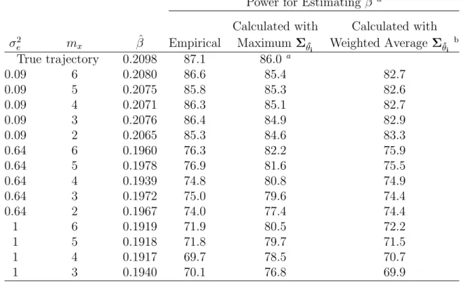
TABLE 2.2: Power for estimating _β by maximum number of data collection points (_mx) and size of σe2 - linear trajectory

Power for Estimating _β a

Calculated with Calculated with σ2

e mx βˆ Empirical MaximumΣ_θˆ_i Weighted Average Σˆ_θ_i b

True trajectory 0.2098 87.1 86.0 a

0.09 6 0.2080 86.6 85.4 82.7

0.09 5 0.2075 85.8 85.3 82.6

0.09 4 0.2071 86.3 85.1 82.7

0.09 3 0.2076 86.4 84.9 82.9

0.09 2 0.2065 85.3 84.6 83.3

0.64 6 0.1960 76.3 82.2 75.9

0.64 5 0.1978 76.9 81.6 75.5

0.64 4 0.1939 74.8 80.8 74.9

0.64 3 0.1972 75.0 79.6 74.4

0.64 2 0.1967 74.0 77.4 74.4

1 6 0.1919 71.9 80.5 72.2

1 5 0.1918 71.8 79.7 71.5

1 4 0.1917 69.7 78.5 70.7

1 3 0.1940 70.1 76.8 69.9

a_{Calculated with}_Σ θi

a_β _{was estimated using the two-step inferential approach (Tsiatis et al. 1995). Empirical power} was based on 1000 simulations, each with 100 subjects per arm. Minimum follow-up time is 0.75 years (9 months), and maximum follow-up time is 2 years. The event time is simulated from an exponential distribution with λ₀ = 0.85, α = 0.3, γ = 0.1, β = 0.2, E(θ₀_i) = 0, E(θ₁_i) = 3.,

V ar(θ₀_i) = 1.2, Var(θ₁_i) = 0.7, and Cov(θ₀_i, θ₁_i) = 0 (the same simulated data used in Row 4 of Table 2.1).

b_{Power based on weighted average of}_Σ_ˆ θi.

inferential approach yields nearly unbiased estimates of the longitudinal eﬀect. The

number of data collection points did not seem to be critical when the trajectory is

linear as long as each subject had at least two measurements of the longitudinal data.

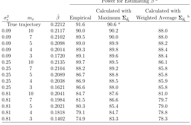
There is a slight decrease in power when _mx <5 and σ2e is large. When the trajectory

is quadratic,_mx plays a more important role. The power for estimatingβ decreases as

mx decreases. Smaller numbers of measurements (mx < 4) can also lead to a biased

estimate of the longitudinal effect and result in a significant loss of power. The effect

(36)

TABLE 2.3: Power for estimating _β by maximum number of data collection points (_mx) and size of σe2 - quadratic trajectory

Power for Estimating _β a

Calculated with Calculated with σ2

e mx βˆ Empirical MaximumΣ_θˆ_i Weighted Average Σ_θˆ_i b

True trajectory 0.2212 91.6 90.6 a

0.09 10 0.2117 90.0 90.2 88.0

0.09 7 0.2102 89.5 90.0 88.0

0.09 5 0.2098 89.0 89.9 88.2

0.09 4 0.2014 89.3 89.8 88.4

0.09 3 0.1720 89.1 89.6 88.4

0.25 10 0.2135 89.7 89.5 86.1

0.25 7 0.2104 88.2 89.2 85.8

0.25 5 0.2089 86.7 88.8 85.8

0.25 4 0.2038 86.9 88.5 85.9

0.25 3 0.1621 86.6 88.0 85.8

0.81 10 0.2041 84.7 87.6 81.0

0.81 7 0.1984 81.5 86.6 79.7

0.81 5 0.2021 80.3 85.4 79.0

0.81 4 0.1818 79.1 84.7 78.8

0.81 3 0.1402 74.9 83.3 78.3

a_{Calculated with}_Σ θi

a_β _{was estimated with the two-step inferential approach (Tsiatis et al. 1995). Empirical power} was based on 1000 simulations, each with 100 subjects per arm. Minimum follow-up time is 0.75 years (9 months), and maximum follow-up time is 2 years. The event time is simulated from an exponential distribution with λ₀ = 0.85, α = 0.3, γ = 0.1, β = 0.22, θ_i = (0, 2.5, 3)T, and

Σθ=diag(1.2, 0.7, 0.8).

b_{Power based on weighted average of}_Σ_ˆ θi.

σ2

e = 0, Σθˆ_i reduces to Σθ, and is unrelated to mx. The eﬀect of mx comes from the

magnitude of reducing the contribution of the within subject variability,_σ2

e. If we have

a very accurate and reliable measurement instrument, we can reduce the number of

repeated measurements and can still obtain unbiased estimates and maximum power.

The power calculation under the assumption of known Σθ or perfect data collection

(maximum Σ_θˆ

i) can result in a signiﬁcant over-estimate of the power especially when

σ2

e is large. We next demonstrate that if we use the weighted average ofΣθˆ_i’s, we can

(37)

Example 1 from Table 2.2: For the scenario with_σ2

e = 0.64 andmx = 2, we observed

that the mean measurement time for the subjects who had an event in the simulated

data is about 0.5 years. We used R2 =

⎛ ⎜

⎝ 1 0

1 0_.5

⎞ ⎟

⎠ to calculateΣˆ_θ instead of setting

R2 =

⎛ ⎜

⎝ 1 0

1 2

⎞ ⎟

⎠, which assumes that the 2nd measurement was taken at 2 years. As a

result, the power based on formula (2.4) changed from 77.4% to 74.4%, which is much

closer to the empirical power of 74.0%. We used the mean measurement time in the

non-censored subjects, because the power calculation is mainly based on the number

of events. In practice, we need to make certain assumptions about _tk based on the

median survival and length of the follow-up period.

Example 2 from Table 2.3: For demonstration, we chose the scenario with _σ2

e =

0_.81 and _mx = 4. In this example, the 2nd measurement was taken at 0.45 years

(on average) in subjects who had only 2 measurements. For subjects who had more

than 2 measurements, longitudinal data was collected at scheduled time points of 0,

0.5, 1, and 1.5. Therefore, R2 =

⎛ ⎜

⎝ 1 0 0

1 0_.45 0_.20

⎞ ⎟

⎠, R3 =

⎛ ⎜ ⎜ ⎜ ⎜ ⎝

1 0 0

1 0_.5 0_.25

1 1 1

⎞ ⎟ ⎟ ⎟ ⎟ ⎠, and

R4 =

⎛ ⎜ ⎜ ⎜ ⎜ ⎜ ⎜ ⎜ ⎝

1 0 0

1 0_.5 0_.25

1 1 1

1 1_.5 2_.25

⎞ ⎟ ⎟ ⎟ ⎟ ⎟ ⎟ ⎟ ⎠

. A weighted average of the Σ_θˆ_i’s was calculated based on

formula (2.11). The resulting power is 78.8% instead of 84.7%, which is close to the

empirical power of 79.1%.

For trajectories that are quadratic or higher, it is important to schedule data

Design considerations for complex survival models