08113128.pdf

C

entral to the looming paradigm shift toward data-in-tensive science, machine-learning techniques are be-coming increasingly important. In particular, deep learn-ing has proven to be both a major breakthrough and an extremely powerful tool in many fields. Shall we embrace deep learning as the key to everything? Or should we resist a black-box solution? These are controversial issues within the remote-sensing community. In this article, we analyze the challenges of using deep learning for remote-sensing data analysis, review recent advances, and provide resourc-es we hope will make deep learning in remote sensing seem ridiculously simple. More importantly, we encourage remote-sensing scientists to bring their expertise into deep learning and use it as an implicit general model to tackle unprecedented, large-scale, influential challenges, such as climate change and urbanization.

MOTIVATION

Deep learning is the fastest-growing trend in big data analysis and was deemed one of the ten breakthrough technologies of 2013 [1]. It is characterized by neural networks (NNs) in-volving usually more than two hidden layers (for this rea-son, they are called deep). Like shallow NNs, deep NNs ex-ploit feature representations learned exclusively from data, instead of handcrafting features that are designed based mainly on domain-specific knowledge. Deep learning research has been extensively pushed by Internet compa-nies, such as Google, Baidu, Microsoft, and Facebook, for several image analysis tasks, including image indexing, seg-mentation, and object detection.

Based on recent advances, deep learning is proving to be a very successful set of tools, sometimes able to surpass

Digital Object Identifier 10.1109/MGRS.2017.2762307 Date of publication: 27 December 2017

Deep Learning

in Remote Sensing

XIAO XIANG ZHU, DEVIS TUIA, LICHAO MOU, GUI-SONG XIA,

LIANGPEI ZHANG, FENG XU, AND FRIEDRICH FRAUNDORFER

even humans in solving highly computational tasks (con-sider, e.g., the widely reported Go match between Google’s AlphaGo artificial intelligence program and the world Go champion Lee Sedol). Based on such exciting successes, deep learning is increasingly the model of choice in many application fields.

For instance, convolutional NNs (CNNs) have proven to be good at extracting mid- and high-level abstract features from raw images by interleaving convolutional and pooling layers (i.e., by spatially shrinking the feature maps layer by layer). Recent studies indicate that the feature representa-tions learned by CNNs are highly effective in large-scale

image recognition [2]–[4], object detection [5], [6], and se-mantic segmentation [7], [8]. Furthermore, recurrent NNs (RNNs), an important branch of the deep learning family, have demonstrated significant achievement on a variety of tasks involved in sequential data analysis, such as action recognition [9], [10] and image captioning [11].

In the wake of this success and thanks to the increased availability of data and computational resources, the use of deep learning is finally taking off in remote sensing as well. Remote-sensing data present some new challenges for deep learning, because satellite image analysis raises unique is-sues that pose difficult new scientific questions.

◗ Remote-sensing data are often multimodal, e.g., from optical (multi- and hyperspectral), Lidar, and synthetic aperture radar (SAR) sensors, where the imaging geom-etries and content are completely different. Data and in-formation fusion uses these complementary data sources in a synergistic way. Already, prior to a joint information extraction, a crucial step involves developing novel archi-tectures to match images taken from different perspec-tives and even different imaging modalities, preferably without requiring an existing three-dimensional (3-D) model. Also, in addition to conventional decision fusion, an alternative is to investigate the transferability of trained networks to other imaging modalities.

◗ Remote-sensing data are geolocated, i.e., they are naturally located in the geographical space. Each pixel corresponds to a spatial coordinate, which facilitates the fusion of pixel information with other sources of data, such as geograph-ic information system layers, geotagged images from so-cial media, or simply other sensors (as just discussed). On the one hand, this allows tackling data fusion with non-traditional data modalities. On the other hand, it opens the field to new applications, such as picture localization, location-based services, and reality augmentation.

◗ Remote-sensing data are geodetic measurements in which quality is controlled. This enables us to retrieve geoparam-eters with confidence estimates. However, unlike purely data-driven approaches, the role of prior knowledge con-cerning the sensors’ adequacy and data quality becomes especially crucial. To retrieve topographic information, e.g., even at the same spatial resolution, interferograms acquired using a single-pass SAR system are considered to be more reliable than the ones acquired in a repeat-pass manner.

◗ The time variable is becoming increasingly important in the field. The Copernicus program guarantees continuous data acquisition for decades; e.g., Sentinel-1 images the en-tire Earth every six days. This capability is triggering a shift from individual image analysis to time-series processing. Novel network architectures must be developed to opti-mally exploit the temporal information jointly with the spatial and spectral information of these data.

◗ Remote sensing also faces the “big data” challenge. In the Copernicus era, we are dealing with very large and ever-growing data volumes, often on a global scale. Even if they were launched in 2014, e.g., Sentinel satellites have already acquired about 25 PB of data. The Coperni-cus concept calls for global applications, i.e., algorithms must be fast enough and sufficiently transferrable to be applied for the whole Earth surface. However, these data are well annotated and contain plenty of metadata. Hence, in some cases, large training data sets might be generated (semi)automatically.

◗ In many cases, remote sensing aims at retrieving geo-physical or biochemical quantities rather than detect-ing or classifydetect-ing objects. These quantities include mass movement rates, mineral composition of soils, water constituents, atmospheric trace gas concentrations, and

terrain elevation of biomass. Often, process models and expert knowledge exist and are traditionally used as pri-ors for the estimates. This suggests, in particular, that the dogma of expert-free, fully automated deep learning should be questioned for remote sensing and that physi-cal models should be reintroduced into the concept, as, e.g., in the concept of emulators [12].

Remote-sensing scientists have exploited the power of deep learning to tackle these different challenges and insti-gated a new wave of promising research. In this article, we review these advances.

FROM PERCEPTRON TO DEEP LEARNING

The perceptron is the basis of the earliest NNs [13]. It is a bioinspired model for binary classification that aims to mathematically formalize how a biological neuron works. In contrast, deep learning has provided more sophisticated methodologies to train deep NN architectures. In this sec-tion, we recall the classic deep learning architectures used in visual data processing.

AUTOENCODER MODELS

AUTOENCODER AND STACKED AUTOENCODER

An autoencoder (AE) [14] takes an input x!RD and, first, maps it to a latent representation h!RM via a nonlinear mapping:

h=f(Wx+b), (1)

where W is a weight matrix to be estimated during train-ing, b is a bias vector, and f stands for a nonlinear function, such as the logistic sigmoid function or a hyperbolic tangent function. The encoded feature representation h is then used to reconstruct the input x by a reverse mapping, leading to the reconstructed input y:

W h

( ),

f

y= l +bl (2)

where Wl is usually constrained to be the form of W_l=WT, i.e., the same weight is used for encoding the input and de-coding the latent representation. The reconstruction error is defined as the Euclidean distance between x and y that is constrained to approximate the input data x (i.e., mini-mizing x y- ₂2). The parameters of the AE are generally optimized by stochastic gradient descent (SGD).

A stacked AE (SAE) is an NN consisting of multiple lay-ers of AEs in which the outputs of each layer are wired to the inputs of the following one.

SPARSE AUTOENCODER

The conventional AE relies on the dimension of the latent representation h being smaller than that of input x, i.e.,

AE [15] boils down to finding the optimal parameters by minimizing the following loss function:

x y

( ( , , ) ( ,

N J

L 1 i , KL ))

i N

i

j j

M

1 1

b m t t

H

= +

= =

t

/

/

(3)

where J( , ,x yi i _H,_b) _{is an average sum-of-squares error} term, which represents the reconstruction error between the input xi _{and its reconstruction y}i_{.KL( )}

j

t tt is the Kull-back–Leibler (KL) divergence between a Bernoulli random variable with mean t and a Bernoulli random variable with mean :ttj

( ) log (1 )log₁1 . KL j

j j

t t =t _tt + -t _tt

-t _{t t} (4)

KL divergence is a standard function for measuring the similarity between two distributions. In the sparse AE model, the KL divergence is a sparsity penalty term, and m controls its importance. t is a free parameter corresponding to a desired average activation value, and tt indicates the actual average ac-tivation value of hidden neuron hj over the training samples. An activation corresponds to how often a region of the im-age reacts when convolved with a filter. In the first layer, e.g., each location in the image receives a value that corresponds to a linear combination of the original input and the filter ap-plied. The higher such value, the more activated this filter is on that region. When convolved over the whole image, a filter produces an activation map, which is the activation at each lo-cation where the filter has been applied. Similar to the AE, the optimization of a sparse AE can be achieved via SGD.

RESTRICTED BOLTZMANN MACHINE AND DEEP BELIEF NETWORK

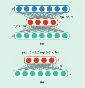
Unlike the deterministic network architectures, such as AEs or sparse AEs, a restricted Boltzmann machine (RBM) (see Figure 1) is a stochastic undirected graphical model consist-ing of a visible layer and a hidden layer. No connections exist within the hidden layer or the input layer. The energy function of an RBM can be defined as follows:

x x x Wx c x b h

( , )h ₂1 (h ),

E = T - T + T + T (5)

where W c, , and b are learnable weights. Here, the input x is also named as the visible random variable, which is denoted as v in the original RBM paper [16]. The joint probability distribution of the RBM is defined as

x h x h

( , ) exp( ( , )),

p =_Z1 -E (6)

where Z is a normalization constant. The form of the RBM makes the conditional probability distribution computa-tionally feasible when x or h is fixed.

The feature representation ability of a single RBM is lim-ited. However, its real power emerges when two or more RBMs are stacked, forming a deep belief network (DBN) [16].

Hinton et al. [16] proposed a greedy approach that trains RBMs in each layer to efficiently train the whole DBN.

CONVOLUTIONAL NEURAL NETWORKS

Supervised deep NNs have come under the spotlight in re-cent years. The leading model is the CNN, which studies the filters performing convolutions in the image domain. Here, we briefly review some successful CNN architectures recently offered for computer vision. For a comprehensive introduction to CNNs, we refer readers to the excellent book by Goodfellow and colleagues [17].

ALEXNET

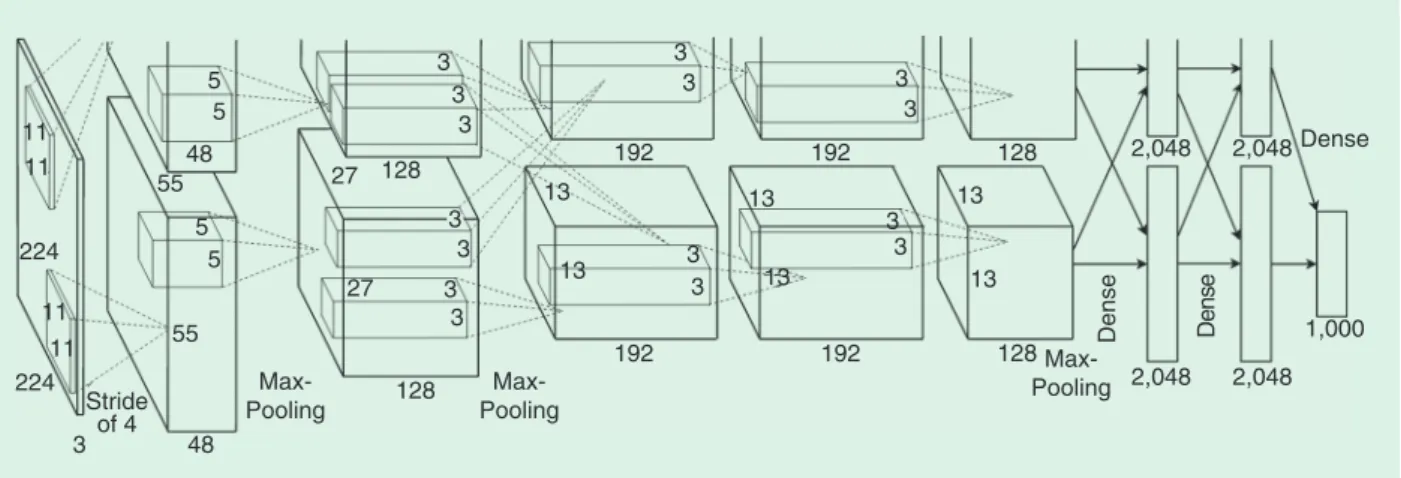
In 2012, Krizhevsky et al. [2] created AlexNet, a “large, deep convolutional neural network” that won the 2012 ImageN-et Large-Scale Visual Recognition Challenge (ILSVRC). The year 2012 is marked as the first year that a CNN was used to achieve a top-five test error rate of 15.4%.

AlexNet (see Figure 2) scaled the insights of LeNet [18] into a deeper and much larger network that could be used to learn the appearance of more numerous and complicated objects. The contributions of AlexNet in-clude the following:

◗ using rectified linear units (ReLUs) as nonlinearity func-tions capable of decreasing training time because a ReLU is several times faster than the conventional hyperbolic tangent function

◗ implementing dropout layers to avoid the problem of overfitting

◗ using data augmentation techniques to artificially increase the size of the training set (and observe a more diverse set of situations); from this, the training patches are translated and reflected on the horizontal and vertical axes.

y

x f (x; Θ, β)

f (h; Θ ′, β′) h

(a)

(b)

p (x, h) = 1/Z exp (–E(x, h))

h W

x

One of the keys of the success of AlexNet is that the model was trained on graphics processing units (GPUs). The fact that GPUs can offer a much larger number of cores than central processing units allows much faster training, which, in turn, allows the use of larger data sets and bigger images.

VGG NETWORKS

The design philosophy of VGG networks (named for Ox-ford University’s Visual Geometry Group) [3] is simplic-ity and depth. In 2014, Simonyan and Zisserman created VGG networks that make use strictly of 3 × 3 filters with stride and padding of 1, along with 2 × 2 max-pooling layers with stride of 2. The main points of VGG networks are that they

◗ use filters with a small receptive field of 3 × 3, rather than larger ones (5 × 5 or 7 × 7, as in Alexnet)

◗ have the same feature map size and number of filters in each convolutional layer of the same block

◗ increase the size of the features in the deeper layers, roughly doubling after each max-pooling layer

◗ use scale jittering as one data augmentation technique during training.

VGG networks are one of the most influential CNN models, as they reinforce the notion that CNNs with deeper architectures can promote hierarchical feature representa-tions of visual data, which, in turn, improves classification accuracy. A drawback is that training such a model from scratch requires large computational power and a very large labeled training set.

RESNET

He et al. [4] pushed the idea of very deep networks even further by proposing the 152-layer ResNet, which won ILS-VRC 2015 with a top-5 error rate of 3.6% and set new re-cords in classification, detection, and localization through a single network architecture. In [4], the authors provide an in-depth analysis of the degradation problem, i.e., that simply increasing the number of layers in plain networks results in higher training and test errors, and they claim

that it is easier to optimize the residual mapping in the ResNet than to optimize the original, unreferenced map-ping in conventional CNNs. The core idea of ResNet is to add shortcut connections that bypass two or more stacked convolutional layers by performing identity mapping. The connections are then added together with the output of stacked convolutions.

FULLy CONVOLUTIONAL NETWORK

The fully convolutional network (FCN) [7] is the most im-portant work in deep learning for semantic segmentation, i.e., the task of assigning a semantic label to every pixel in the image. To perform this task, the output of the CNN must be of the same pixel size as the input (contrary to the single class per image of the aforementioned models). FCN introduces many significant ideas, such as

◗ end-to-end learning of the upsampling algorithm via an encoder/decoder structure that first downsamples the activation’s size and then upsamples it again

◗ using a fully convolutional architecture, which allows the network to take images of arbitrary size as input be-cause there is no fully connected layer at the end that requires a specific size of the activations

◗ introducing skip connections as a way of fusing infor-mation from different depths in the network for the multiscale inference.

Figure 3 shows the FCN architecture.

REMOTE SENSING MEETS DEEP LEARNING

Deep learning is taking off in remote sensing, as shown in Figure 4, which illustrates the number of papers published on the topic since 2014. The exponential increase confirms the rapid surge of interest in deep learning for remote sens-ing. In this section, we focus on a variety of remote-sensing applications that are achieved by deep learning and provide an in-depth investigation from the perspectives of hyper-spectral image analysis, interpretation of SAR images, inter-pretation of high-resolution satellite images, multimodal data fusion, and 3-D reconstruction.

11 11

11 11 224

224

55 55

5 5 5

48

27

27

128

192 192

192 192 128

128 13

13

13

13 13

13 3

3 3

3

3 3

3

3

Max-Pooling

Max-Pooling 2,048 2,048 2,048 2,048

1,000

Max-Pooling 128

3 3

3 3 3 3

5

48 3

Stride of 4

Dense Dens

e

Dense

3

HYPERSPECTRAL IMAGE ANALYSIS

Hyperspectral sensors are character-ized by hundreds of narrow spectral bands. This very high spectral resolu-tion enables us to identify the materials contained in the pixel via spectroscop-ic analysis. Analysis of hyperspectral data is of great importance in many practical applications, such as land cover/use classification or change and object detection. Because high-quality hyperspectral satellite data are becom-ing available (e.g., via the launch of EnMAP, planned for 2020, and the DESIS on the International Space Sta-tion, planned for 2018), hyperspectral

image analysis has been one of the most active research areas within the remote-sensing community over the last decade.

Inspired by the success of deep learning in computer vi-sion, preliminary studies have been carried out on deep learn-ing in hyperspectral data analysis, which brlearn-ings new momen-tum to this field. In the following, we review two application cases, land cover/use classification and anomaly detection.

HyPERSPECTRAL IMAGE CLASSIFICATION

Supervised classification is probably the most active research area in hyperspectral data analysis. There is a vast literature on this topic using conventional supervised machine-learn-ing models, such as decision trees, random forests, and sup-port vector machines (SVMs) [20]. With the investigation of hyperspectral image classification [21], a major finding was that various atmospheric scattering conditions, complicated light-scattering mechanisms, interclass similarity, and in-traclass variability result in the hyperspectral imaging pro-cedure being inherently nonlinear. It is believed that, com-pared to the previously mentioned shallow models, deep learning architectures are able to extract high-level, hierar-chical, and abstract features, which are generally more robust to the nonlinear processing.

The following sections discuss research on hyperspec-tral image classification.

SAE FOR HyPERSPECTRAL DATA CLASSIFICATION A first attempt in this direction can be found in [22], where the authors make use of an SAE to extract hierarchical fea-tures in the spectral domain. Subsequently, in [23], the au-thors employ DBN. Similarly, Tao et al. [24] use sparse SAEs to learn an effective feature representation from input data; then, the learned features are fed into a linear SVM for hy-perspectral data classification.

SUPERVISED CNNs

In [25], the authors train a simple one-dimensional (1-D) CNN that contains five layers—i.e., an input layer, a convolutional layer, a max-pooling layer, a fully connected

layer, and an output layer—and directly classify hyperspec-tral images in the spechyperspec-tral domain.

Makantasis et al. [26] exploited a two-dimensional (2-D) CNN to encode spectral and spatial information, fol-lowed by a multilayer perceptron performing the actual classification. In [27], the authors attempted to carry out the classification of crop types using 1-D CNN and 2-D CNN. They concluded that the 2-D CNNs can outperform the 1-D CNNs, but some small objects in the final clas-sification map provided by 2-D CNNs are smoothed and misclassified. To avoid overfitting, Zhao and Du [28] sug-gest a spectral-spatial-feature-based classification frame-work, which jointly makes use of a local-discriminant embedding-based dimension-reduction algorithm and a 2-D CNN. In [21], the authors propose a self-improving CNN model that combines a 2-D CNN with a fractional-order Darwinian particle swarm optimization algorithm to iteratively select the most informative bands suitable for training the designed CNN. Santara et al. [29] discuss

Forward/Inference

Backward/Learning

Pixelwise PredictionSegmentation g.t.

96

21

21

256 384 384 256

4,096 4,096

FIGURE 3. The FCN architecture [7]. g.t.: ground truth.

71 78

23

3

2014 2015 2016 2017

Publication Years

100+ (Predicted)

(Sept. 2017)

an end-to-end, band-adaptive spectral-spatial-feature-learning network to address the problems of the curse of dimensionality. In [30], to allow a CNN to be appropriately trained using limited labeled data, the authors present a novel pixel-pair CNN to significantly augment the number of training samples.

Following recent vision developments in 3-D CNNs [31], in which the third dimension usually refers to the time axis, such architecture has also been employed in hyperspectral classification. In other words, in a 3-D CNN, convolution operations are performed spatial spectrally, while in 2-D CNNs, they are done only spatially. The authors in [19] in-troduce a supervised, ,2-regularized 3-D CNN-based mod-el (see Figure 5), while the authors of [32] follow a similar idea for spatial-spectral classification.

UNSUPERVISED DEEP LEARNING

To allow less dependence on the existence of large anno-tated collections of labeled data, unsupervised feature extraction is of great interest. The authors of [35] propose an unsupervised convolutional network for learning spec-tral-spatial features using sparse learning to estimate the network weights in a greedy layerwise fashion instead of end-to-end learning. Mou et al. [33], [34] present a network architecture called a fully residual conv-deconv network for un-supervised spectral-spatial feature learning of hyperspec-tral images. They report an extensive study of the filters learned (see Figure 6).

RECURRENT NEURAL NETWORKS FOR HyPERSPECTRAL IMAGE CLASSIFICATION

In [36], the authors propose an RNN model with a new activation function and modified gated recurrent unit for hyperspectral image classification that can effectively analyze hyperspectral pixels as sequential data and then determine information categories via network reasoning (see Figure 7).

ANOMALy DETECTION

In a hyperspectral image, the pixels whose spectral signa-tures are significantly different from the global background pixels are considered anomalies. Because the prior knowl-edge of the anomalous spectrum is difficult to obtain in practice, anomaly detection is usually solved by background modeling or statistical characterization for hyperspectral data. So far, the only attempt to address this problem via deep learning can be found in [37], where Li et al. propose an anomaly detection framework in which a multilayer CNN is trained using the differences in values between neighboring pixel pairs in the reference image as input data. Then, in the test phase, anomalies are detected by evaluating differences between neighboring pixel pairs using the trained CNN.

In summary, deep learning has been widely applied to multi/hyperspectral image classification, and some promising results have been achieved. In contrast, for other hyperspectral data analysis tasks, such as change and anomaly detections, deep learning is just beginning to make its mark [37], [38]. Some potential problems to Hyperspectral

Image

Neighborhood of the Pixel

Vector

3-D Conv.

Pooling _Pooling Logis

tic

Regr essio

n

Label

3-D Conv.

FIGURE 5. A flowchart of the 3-D CNN architecture proposed in [19] for spectral-spatial hyperspectral image classification. Conv.: convolution.

(a) (b)

be further explored include nonlinear spectral unmixing, hyperspectral image enhancement, and hyperspectral time-series analysis.

INTERPRETATION OF SYNTHETIC APERTURE RADAR IMAGES

Over the past several years, many studies related to deep learn-ing for SAR image analysis have been published. Among these, deep learning techniques have been used most in typical ap-plications, including automatic target recognition (ATR), ter-rain surface classification, and parameter inversion. This section reviews some of the relevant studies in this area.

AUTOMATIC TARGET RECOGNITION

SAR ATR is an important application, in particular, for mili-tary surveillance [39]. A standard architecture for efficient ATR consists of three stages: detection, discrimination, and classification. Each stage tends to perform a more compli-cated and refined processing than its predecessor and selects the candidate objects for the next-stage processing. Howev-er, all three stages can be treated as a classification problem and, for this reason, deep learning has made its mark.

Chen and Wang [40] introduced CNNs into SAR ATR and tested them on the standard ATR data set MSTAR[41]. They found the major issue to be the lack of sufficient training samples as compared to optical images. This might cause se-vere overfitting and, therefore, greatly limit the capability of generalizing the model, so data augmentation is employed to counteract overfitting. Chen et al. [42] propose to further remove all fully connected layers from conventional CNNs, which are accountable for most trainable parameters. The final performance is demonstrated as superior compared to conventional CNNs on the MSTAR data set (i.e., a state-of-the-art accuracy of 99.1% in standard operating condition). Extensive experiments have been conducted to test the

generalization capability of the so-called AConvNets, and they have proved to be quite robust in several extended op-erating conditions. The removal of the fully connected lay-ers, originally designed to be trainable classifilay-ers, might be justifiable in this case because the limited number of target types can be seen as the feature templates that the ACon-vNets are extracting.

Many authors have applied CNNs to SAR ATR and tested the results on the MSTAR data

set, e.g., [43]–[46]. Among these studies, the one common find-ing is that data augmentation is necessary and the most critical step for SAR ATR using CNNs. Various augmentation strate-gies have been offered, includ-ing translation, rotation, and interpolation. Cui et al. [47]

introduce DBN to SAR ATR, where stacked RBMs are used to extract features that are then fed to a trainable classifier.

Wagner [48] suggests using a CNN to first extract feature vectors and then feed them to an SVM for classification. The CNN is trained with a fully connected layer, but only the previous activations are used. A systematic data augmenta-tion approach is employed, which includes elastic distor-tions and affine transformadistor-tions. It is intended to mimic typical imaging errors, such as a changing range (which is scale dependent on the depression angle) or an incorrectly estimated aspect angle.

Additional studies applying CNNs to the ATR problem are also of interest. Bentes et al. [49] applied a CNN to ship– iceberg discrimination, tested on TerraSAR-X StripMap im-ages. Schwegmann et al. [50] applied a specific type of deep NNs, highway networks, to the discrimination of ships in SAR imagery and achieved promising results. Ødegaard et al.

Hyperspectral Image Classification Map

Input Layer Recurrent Layer + Batch Normalization + PRetanh Fully Connected Layer Softmax Layer

One Pixel

xk–1

xk+1 xk

p h

GRU

p h

GRU

p h

GRU

Network

FIGURE 7. The RNN proposed for the hyperspectral image classification task in [36]. GRU: gated recurrent unit; PRetanh: parametric recti-fied tanh.

SAR ATR IS AN IMPORTANT APPLICATION, IN

[51] applied a CNN to detect ships in a harbor background in SAR images; to address the issue of a lack of training samples, they employed a simulation software to generate simulated data for training. Song et al. [52] follow this idea, introduc-ing a deep generative NN for SAR ATR. A generative decon-volutional NN is first trained to generate a simulated SAR image from a given target la-bel, while a feature space is simultaneously constructed in the intermediate layer. A CNN is then trained to map an in-put SAR image to the feature space. The goal is to develop an extended ATR system capa-ble of interpreting a previously unseen target in the context of all known targets.

TERRAIN SURFACE CLASSIFICATION

When terrain surface classification uses SAR, in particular polarimetric SAR (PolSAR), data meet another important application in radar remote sensing. This is very similar to the task of image segmentation in computer vision. Conven-tional approaches are based mostly on pixelwise polarimet-ric target decomposition parameters [54]. They hardly con-sider the spatial patterns, which convey rich information in high-resolution SAR images [55]. Deep learning provides a tool for automatically extracting features that represent spa-tial patterns as well as polarimetric characteristics.

One large stream of studies employs at least one type of unsupervised generative graphical models, such as the DBN, SAE, or RBM. Xie et al. [56] first introduced multilayer feature learning for PolSAR classification; here, an SAE is employed to extract useful features from a channel PolSAR image.

Geng et al. [57] proposed a deep convolutional AE (DCAE) to extract features and conduct classification automatically. The DCAE consists of a handcrafted first layer of convolu-tion that contains kernels, such as gray-level co-occurrence matrix and Gabor filters, and a handcrafted second layer of scale transformation that integrates correlated neighbor pixels. The remaining layers are trained SAEs. This ap-proach was tested on high-resolution, single-polarization

TerraSAR-X images. Geng et al. [58] later presented a simi-lar framework, deep supervised and contractive NN, for SAR image classification; this framework additionally in-cludes the histogram of oriented gradient descriptors as handcrafted kernels. The trainable AE layers employ a supervised penalty that captures the relevant information between features and labels, as well as a contractive restric-tion that enhances local invariance. An interesting finding of Geng et al. [58] is that speckle reduction yields the worst performance, and the authors suspect that speckle reduc-tion might smooth out some useful informareduc-tion.

Lv et al. [59] tested DBN on urban land use and land cover classification using PolSAR data. Hou et al. [60] proposed an SAE combined with superpixels for PolSAR image classifica-tion. Here, multiple AE layers are trained on a pixel-by-pixel basis, and superpixels are formed based on Pauli-decomposed pseudocolor images. The output of the SAE is used as a feature in the final step for k-nearest neighbor clustering of superpix-els. Zhang et al. [61] applied a stacked sparse SAE to PolSAR image classification, while Qin et al. [62] applied adaptive boosting of RBMs to PolSAR image classification. Zhao et al. [63] proposed discriminant DBN for SAR image classification; here, the discriminant features are learned by combining en-semble learning with a DBN in an unsupervised manner.

Jiao and Liu [64] presented a deep stacking network for PolSAR image classification, which mainly takes advantage of fast Wishart distance calculation through linear projec-tion. The proposed network aims to perform a k-means clustering/classification task where Wishart distance is used as the similarity metric.

The other stream of studies involves CNNs. Zhou et al. [65] applied CNNs to PolSAR image classification; here, a covariance matrix is extracted as six real-channel data in-put. Duan et al. [66] suggested replacing the conventional pooling layer in CNNs by a wavelet-constrained pooling layer. The so-called convolutional-wavelet NN is then used in conjunction with superpixels and a Markov random field (MRF) to produce the final segmentation map.

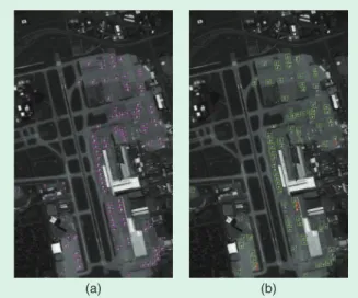
Zhang et al. [53] described a complex-valued (CV) CNN (see Figure 8) specifically designed to process complex values in PolSAR data, i.e., the off-diagonal elements of coherency or covariance matrix. The CV CNN not only takes complex numbers as input but also employs complex weights and

a + jb

W ∈

Conv. Layers ∈ Pooling Layers ∈ Conv. Layers ∈

Output Layer ∈

Fully Connected Layers ∈

Pooling Layers ∈

FIGURE 8. The structure of a CV CNN (adapted from [53]). WhEN TERRAIN SURFACE

CLASSIFICATION USES SAR, IN PARTICULAR

complex operations throughout different layers. A CV back-propagation algorithm is also developed to train it. Figure 9 shows an example of PolSAR classification using a CV CNN.

PARAMETER INVERSION

The authors of [67] applied CNNs to estimate ice concen-tration using SAR images during melt season. The labels were produced by visual interpretation by ice experts and tested on dual-polarized RadarSat-2 data. Because the prob-lem considered is regression of a continuous value, the loss function is selected as mean-squared error. The final results suggest that CNNs can produce a more detailed result than operational products.

INTERPRETATION OF HIGH-RESOLUTION SATELLITE IMAGES

SCENE CLASSIFICATION

Scene classification, which aims to automatically assign a semantic label to each scene image, has been an active re-search topic in the field of high-resolution satellite images in past decades [68]–[74]. As a key problem in the interpre-tation of satellite images, it has widespread applications, including object detection [75], [76], change detection [77], urban planning, and land resource management. However, due to the high spatial resolutions, different scene images may contain the same kinds of objects or share similar spa-tial arrangement, e.g., both residenspa-tial areas and commer-cial areas may contain buildings, roads, and trees, but they are two different scene types. Therefore, the great variations in the spatial arrangements and structural patterns make scene classification a considerably challenging task.

Generally, scene classification can be divided into two steps: feature extraction and classification. With the grow-ing number of images, traingrow-ing a complicated nonlinear

classifier is time consuming. Hence, extracting a holistic and discriminative feature representation is the most sig-nificant step for scene classification. Traditional approach-es are most often based on the bag-of-visual-words (BoVW) model [78], [79], but their potential for improvement has been limited by the ability of experts to design the feature extractor and the expressive power encoded.

The deep arhitectures discussed in the “Convolutional Neural Networks” section have been applied to the scene classification problem of high-resolution satellite images and led to state-of-the-art performance [71], [74], [80]–[87]. As deep learning is a multilayer feature-learning architec-ture, it can learn more abstract and discriminative semantic features as the depth grows and achieve far better classifica-tion performance compared to midlevel approaches. In this section, we summarize the existing deep learning-based methods according to the following three categories:

◗ Using pretrained networks: The deep CNN pretrained on a

natural image data set, e.g., OverFeat [88] and GoogLeNet [89], has led to impressive results on the scene classifica-tion of high-resoluclassifica-tion satellite images by directly ex-tracting the features from the intermediate layers to form global feature representations [81]–[83], [87]; e.g., [74], [81], and [82] directly use the features from the fully con-nected layers as the input of the classifier, while [83] takes the CNN as a local feature extractor and combines it with feature coding techniques, such as BoVW [78] and vector of locally aggregated descriptors (VLAD), to generate the final image representation.

◗ Making a pretrained model adapt: Making a pretrained

model adapt to the specific conditions observed in a data set under study, one can decide to fine-tune it on a smaller labeled data set of satellite images. The authors of [82] and [86], e.g., fine-tune some high-level layers of the GoogLeNet [89] using the University of California–Merced

(a) (b)

Potato Fruit Oats Beets Barley Onions Wheat Beans Peas Maize

Flax Rapeseed

Grass Lucerne

(UC Merced) data set [90] (see the “Remote-Sensing Data for Training Deep Learning Models” section), thus obtaining better results than when directly using only the pretrained CNNs. This can be explained, because the features learned are more oriented to the satellite images after fine-tuning, which can help exploit the intrinsic characteristic of satellite images. Nonetheless, compared with the natural image data set consisting of more than 10 million samples, the scales of public satellite image data sets (i.e., UC Merced data set [90], RSSCN7 [80], and WHU-RS19 [91]) are fairly small, e.g., up to several thousands, for which we cannot fine-tune whole CNNs to make them more adaptive to satellite images.

◗ Training new networks: In addition to the previous two ways

to use deep learning methods for classifying satellite im-ages, some researchers train the network from scratch us-ing satellite images. The authors of [82] and [86], e.g., train the networks by using only the existing satellite image data set, which suffers a drop in classification accuracy com-pared with using the pretrained networks as global feature extractors or fine-tuning the pretrained networks. The rea-son lies in the fact that large-scale networks usually contain millions of parameters to be learned. Thus, training them using small-scale satellite image data sets will easily cause overfitting and local minimum problems. Consequently, some construct a new smaller network and train it from scratch using satellite images to better fit the satellite data [80], [84], [85], [92]. However, such small-scale networks are often easily oriented to the training images, and the generalization ability decreases. For each satellite data set, the network needs to be retrained.

OBJECT DETECTION

Object detection is another important task in the interpre-tation of high-resolution satellite images [93]: one wishes

to localize one or more specific ground objects of interest (such as a building, vehicle, or aircraft) within a satellite image and predict the corresponding categories, as shown in Figure 10. Due to the powerful ability of learning high-level (more abstract and semantically meaningful) feature repre-sentations, deep CNNs are being explored in object-detec-tion systems in contrast to the more tradiobject-detec-tional methods followed by a classifier based on handcrafted features [94], [95]. Here, we review most existing works using CNNs for both specific and generic object detection.

Jin and Davis [96] proposed a vector-guided vehicle detection approach for IKONOS satellite imagery using a morphological shared-weight NN that learns the implicit vehicle model and incorporates both spatial and spectral characteristics and classifies pixels into vehicles and nonve-hicles. To address the problem of large-scale variance of ob-jects, Chen et al. [97] suggested a hybrid deep CNN model for vehicle detection in satellite images; this model divides all feature maps of the last convolutional and max-pooling layer of the CNN into multiple blocks of variable-receptive-field size or pooling size to extract multiscale features. Jiang et al. [98] proposed a CNN-based vehicle detection ap-proach, wherein a graph-based superpixel segmentation is used to extract image patches and a CNN model is trained to predict whether a patch contains a vehicle.

A few detection methods transfer the pretrained CNNs for object detection. Zhou et al. [99] presented a weakly supervised learning framework to train an object detector; here, a pretrained CNN model is transferred to extract high-level features of objects, and the negative bootstrap-ping scheme is incorporated into the detector training process to provide faster convergence of the detector. Zhang et al. [100] advanced a hierarchical oil tank detec-tor, which combines deep surrounding features extract-ed from the pretrainextract-ed CNN model with local features (histogram of oriented gradients [101]). The candidate regions are selected by an ellipse and line segment detec-tor. Salberg [102] proposed extracting features from the pretrained AlexNet model and applying the deep CNN features for automatic detection of seals in aerial images. Ševo and Avramovic´ [103] suggested a two-stage ap-proach for CNN training and developed an automatic object-detection method based on a pretrained CNN, where the GoogLeNet is first fine-tuned twice on the UC Merced data set using different fine-tuning options and then the fine-tuned model is used for sliding-window object detection. To address the problem of orientation variations of objects, Zhu et al. [104] have employed the pretrained CNN features that are extracted from com-bined layers and implemented orientation-robust object detection in a coarse localization framework.

Zhang et al. [105] proposed a weakly supervised learn-ing approach uslearn-ing coupled CNNs for aircraft detection. The authors employed an iterative, weakly supervised framework that simply requires image-level training data to automatically mine and augment the training data set

(a) (b)

from the original image, which can dramatically decrease human labor. A coupled CNN model, composed of a can-didate region proposal network, and a localization net-work were developed to generate region proposals and lo-cate aircraft simultaneously, which is suitable and effective for large-scale, high-resolution satellite images.

For enhancing the performance of generic object detec-tion, Cheng et al. [76] proposed an effective approach to learning a rotation-invariant CNN (RICNN) to improve in-variance to object rotation. In their paper, they add a new rotation-invariant layer to the off-the-shelf AlexNet model. The RICNN is learned by optimizing a new object function, including an additional regularization constraint that en-forces the training samples before and after being rotated to share similar features and guarantee the rotation-invariant ability of the RICNN model.

Finally, several papers considering methods other than CNNs exist. Tang et al. [106] offered a compressed-domain ship detection framework combined with SDA and an ex-treme learning machine (ELM) [107] for optical spaceborne images. Two SDA models are employed for hierarchical ship feature extraction in the wavelet domain, which can yield more robust features under changing conditions. The ELM was introduced for efficient feature pooling and classifica-tion, making the ship detection accurate and fast. Han et al. [108] advanced an effective object-detection framework, exploiting weakly supervised learning and DBNs. The sys-tem requires only weak labels to identify the presence of an object in the whole image and significantly reduces the labor of manually annotating training data.

IMAGE RETRIEVAL

Remote-sensing image retrieval aims at retrieving images having a similar visual content with respect to a query image from a database [109]. A common image-retrieval system needs to compute image similarity based on im-age feature representations, and thus the performance of a retrieval depends to a large degree on the descriptive capability of image features. Building image representa-tion via feature coding methods (e.g., BoVW and VLAD) using low-level handcrafted features has been proven to be very effective in aerial image retrieval [109], [110]. Nev-ertheless, the discriminative ability of low-level features is very limited, and thus it is difficult to achieve substan-tial performance gain. Recently, a few works have investi-gated extracting deep feature representations from CNNs. Napoletano [111] extracts deep features from the fully connected layers of the pretrained CNN models, and the deep features prove to perform better than low-level fea-tures regardless of the retrieval system. Zhou et al. [112] proposed a CNN architecture followed by a three-layer perceptron, which is trained on a large remote-sensing data set and able to achieve remarkable performance even with low-dimensional deep features. Jiang et al. [113] present a sketch-based satellite-image-retrieval method that involves learning deep cross-domain features, which

enables the retrieval of satellite images with hand-free sketches only.

Although there is still a lack of sufficient study in terms of exploiting deep learning approaches for remote-sensing image retrieval at present, considering the great potential for learning high-level features with deep learning meth-ods, we believe that more deep learning-based image- retrieval systems will be developed in the near future. It is also worth noticing how feedback from users is integrated into the deep learning retrieval scheme.

MULTIMODAL DATA FUSION

Data fusion is one of the fast-moving areas of remote sensing [114]–[116]. Due to recent increases in the availability of sensor data, using big and heterogeneous data to study environmen-tal processes has become more tangible. Of course, when data are big and relations to be

un-veiled are complex, one would favor high-capacity models. In this respect, deep NNs are natural candidates to tackle the challenges of modern data fu-sion in remote sensing. In this section, we review three areas of remote-sensing image analy-sis where data fusion tasks have been approached with deep

learning: pansharpening, feature and decision-level fusion, and fusion of heterogeneous sources.

PANSHARPENING AND SUPERRESOLUTION

Pansharpening is the task of improving the spatial resolu-tion of multispectral data by fusing these with data char-acterized by sharper spatial information. It is a special instance of the more general problem of superresolution. Traditionally, the field was dominated by works fusing mul-tispectral data with panchromatic bands [117], but more re-cently it has been extended to thermal [118] or hyperspec-tral images [119]. Most techniques rely either on projective methods, sparse models, or pyramidal decompositions. Using deep NNs for pansharpening multispectral images is certainly an interesting concept, because most images ac-quired by satellite such as the WorldView series or Landsat come with a panchromatic band. In this respect, training data are abundant, which is in line with the requirements of modern CNNs.

A first attempt in this direction can be found in [120], where the authors use a shallow network to upsample the intensity component obtained after the intensity, hue, and saturation of color images [red, green, blue (RGB)]. Once the multispectral bands have been upsampled with the CNN, a traditional Gram–Schmidt transform is used to perform the pansharpening. The authors use a data set of QuickBird images for their analysis. Even though this is interesting, in [120], the authors simply replace one operation (the nearest neighbor or bicubic convolution) with a CNN.

In [121], the authors propose using a CNN to learn the pansharpening transform end to end, i.e., letting the CNN perform the whole pansharpening process. In their CNN, they stack upsampled spectral bands with the panchromat-ic band and then learn, for each patch, the high resolution values of the central pixel.

In [122], the authors use a superresolution CNN trained on natural images [123] as a pretrained model and fine-tune it on a data set of hyperspectral images. By doing so, they make an attempt at transfer learning [124] between the domains of color (three bands, large bandwidths) and hyperspectral images (many bands, narrow bandwidths). Fine-tuning existing architectures that have been trained on massive data sets with very large models is often a rel-evant solution, because one makes use of discriminative strong features and injects only task-specific knowledge.

In [125], the authors present an upsampling of the pan-chromatic band via a stack of AEs: the model is trained to predict the full-resolution panchromatic image from a downsampled version of itself (at the resolution of the mul-tispectral bands). Once the model is trained, the multispec-tral bands are fed into the model one by one and thereby upsampled using the data relationships learned from the panchromatic images.

FEATURE- AND DECISION-LEVEL FUSION FOR IMAGE CLASSIFICATION

Most of the current remote-sensing literature dealing with deep NNs studies the problem of image classification, i.e., the task of assigning each pixel in the image to a given se-mantic class (land use, land cover, damage level, and so forth). In the following, we review recent approaches deal-ing with image classification problems, mostly at very high resolution, using two strategies: feature-level fusion and decision-level fusion. In the last part of this section, we re-view works using different data sources to tackle separate but related predictive tasks, or multitask problems.

FeAture-level Fusion

Feature-level fusion uses multiple sources simultaneously in a network. Like most image-processing techniques, deep NNs use d-dimensional inputs. A very simple way of using multiple data sources in a deep network is to stack them, i.e., to concatenate the image sources into a single data cube to be

processed. The filters learned by the first layer of the network will, therefore, depend on a stack of different sources. Stud-ies considering this straightforward extension of NNs are nu-merous and, in [126], the authors compared networks trained on RGB data (fine-tuned from existing architectures) with networks including a digital surface model (DSM) channel, using the 2015 Data Fusion Contest data set over the city of Zeebruges [127] (data are available from [188]; also see the “Remote-Sensing Data for Training Deep Learning Models” section). They use the CNN as a feature extractor and then use the features to train an SVM, predicting a single semantic class for the entire patch. They then apply the classifier in a sliding-window manner.

Parallel research has considered spatial structures in the network by training architectures predicting all labels in the patch instead of a single label to be attributed to the central pixel. By doing so, spatial structures are inherently included in the filters. Fully convolutional and deconvolutional ap-proaches are natural candidates for such a task: in the first, the last fully connected layer is replaced with a convolutional layer (see [88]) to have a downsized patch prediction that then needs to be upsampled. In the second, a series of de-convolutions (transposed de-convolutions [7], [8]) are learned to upsample the convolutional fully connected layer. Both approaches have been compared in [92] using the Interna-tional Society for Photogrammetry and Remote Sensing (IS-PRS) Vaihingen and Potsdam benchmark data sets (available in [189]; also see the “Remote-Sensing Data for Training Deep Learning Models” section),stacking color infrared (CIR) and normalized digital elevation models. The archi-tectures are compared and some zoomed results are reported in Figures 11 and 12, respectively. Other strategies for spatial upsampling have been proposed in recent literature, includ-ing the direct use of upsampled activation maps as features to train the final classifier [128]. In [129], the authors stud-ied the possibility of visualizing uncertainty of predictions (applying the model of [130]). They stacked CIR, DSM, and normalized DSM data as inputs to the CNN.

In addition to dense predictions, other strategies have been presented to include spatial information in deep NNs. For example, the authors of [58] extract different types of spatial filters and stack them in a single tensor, which is then used to learn a supervised stack of AEs. They apply their models on the classification of SAR images, so

Downsampling Upsampling Prediction

Input

the fusion here is to be considered between different types of spatial information. The NN is then followed by a condi-tional random field (CRF) to decrease the effect of speckle noise inherent in SAR images. In [131], the authors pres-ent a model that learns combinations of spatial filters ex-tracted from hyperspectral image bands and DSMs. Even if the model is not a traditional deep network, it learns a sequence of recombinations of filters, thereby extracting higher-level information in an automatic way as deep NNs do, i.e., it learns the right filter parameters (along with their combinations) instead of learning the filter coeffi-cients themselves.

Data fusion is also a key component in change detection, where one wishes to extract joint features from a bitempo-ral sequence. The aim is to learn a joint representation in which both (coregistered) images can be compared. This area is especially interesting when methods can align data from multiple sensors (see [132] and [133]). Three studies employ deep learning to this end:

◗ In [134], the authors present a model that learns a joint representation of two images with DBNs. Feature vec-tors issued from the two image acquisitions are stacked and used to learn a representation, where changes stand out more clearly. Using such representation, changes are more easily detected by image differencing. This approach

is applied on optical images from the Chinese GaoFen-1 satellite and WorldView-2.

◗ In [135], the joint representation is learned via a stack of AEs using the single temporal acquisitions at each end of the encoder–decoder system. By doing so, they learn a representation useful for change detection at the bot-tleneck of the system (i.e., in the middle). The authors show the versatility of their approach by applying it to several data sets, including pairs of optical and SAR im-ages, and an example performing change detection be-tween optical and SAR images.

◗ More recent work addresses the transferability of deep learning for change detection, while analyzing data of long time series for large-scale problems. In [38], e.g., the authors make use of an end-to-end RNN to solve the multi/hyperspectral change detection task, because RNN is well known to be good at processing sequential data. In their framework, an RNN based on long short-term memory is employed to learn joint spectral feature rep-resentations from a bitemporal image sequence. In addi-tion, the authors show that their network can detect mul-ticlass changes and has a good transferability for change detection in a new scene without fine-tuning. The au-thors of [136] introduce an RNN-based transfer-learning approach to detect annual urban dynamics of four cities

Image nDSM GT CNN-PC CNN-SPL CNN-FPL

(Beijing, New York, Melbourne, and Munich) from 1984 to 2016, using Landsat data. The main challenge here is that training data in such a large-scale and long-term image sequence are very scarce. By combining RNN and transfer learning, the authors are able to transfer the fea-ture representations learned from a few training samples to new target scenes directly. Some zoomed results are reported in Figure 13.

Another view of feature fusion involves NNs fusing fea-tures obtained from different inputs: two (or more) networks are trained in parallel, and their activations are then fused at a later stage, e.g., by feature concatenation. The author of [137] studies a solution in this direction that fuses two CNNs: the first considers CIR images of the Vaihingen data set and passes them through the pretrained VGG network to learn color features, while the second considers the DSM and learns a fully connected network from scratch. Both models’ features are then concatenated, and two randomly initialized, fully connected layers are learned from this concatenation. A similar logic is also followed in [138], where the authors present a model that learns a fully connected layer perform-ing the fusion between networks learned at different spatial scales. They apply their model to the tasks of buildings and road detection. In [139], the authors train a two-stream CNN with two separate yet identical convolutional streams that process the PolSAR and hyperspectral data in parallel and only fuse the resulting information at a later convolutional layer for the purpose of land cover classification. With a simi-lar network architecture and contrastive loss function, the authors of [140] present a model that learns a network for the

identification of corresponding patches in SAR and optical imagery of urban scenes.

Decision-level Fusion

Decision-level fusion fuses CNN (and other) outputs. While the works reviewed previously use a single network to learn the semantics of interest all at once (either by extracting relevant features or by learning the model end to end), an-other series of works has studied ways of performing deci-sion fudeci-sion with deep learning. Even though the distinction between these and the models reviewed previously might seem artificial, here we review approaches including an explicit fusion layer between land cover maps. We distin-guish between two families of approaches, depending on whether the decision fusion is performed as a postprocess-ing step or learned.

◗ Fusing semantic maps obtained with CNNs: In this case,

dif-ferent models predict the classes, and their predictions are then fused. Two works are particularly notable in this respect. On the one hand [141], the authors fuse a classi-fication map obtained by a CNN with another obtained by a random forest classifier trained using handcrafted features. Both models use CIR, DSM, and normalized DSM inputs from the Vaihingen data set. The two maps are fused by multiplication of the posterior probabili-ties, and an edge-sensitive CRF is also learned on top to improve the quality of the final labeling. On the other hand, the authors in [133] consider the learning of an ensemble of CNNs and then averaging their predic-tions: their proposed pipeline has two main streams,

DOY: 1985–225

Zone: Munich Airpor

t

DOY: 1986–196 DOY: 1990–223 DOY: 2014–161

Urban Bare Land Water Vegetation Cover Cloud

one processing the CIR data and another processing the DSM. They train several CNNs, using them as inputs for the activation maps of each layer of the main model as well as one fusing the CIR and DSM main streams, as in [137]. By doing so, they obtain a series of land cover maps to nourish the ensemble, which improves perfor-mances by considering classifiers issued from different data sources and levels of abstraction. Compared to the previous model discussed in this section, this model has the advantage of being entirely learned in an end-to-end fashion, but it also incurs an extreme computational load and a complex architecture involving many skip connections and fusion layers.

◗ Decision fusion learned in the network: This is an

alterna-tive to an ad hoc fusion (multiplication or averaging of the posterior maps), in which one may learn the optimal fusion. In [142], the authors perform the fusion between two maps obtained by pretrained models by learning a fusion network based on residual learning [4] logic. In their architecture, they learn how to correct the average fusion result by learning extra coefficients favoring one or the other map. Their results show that such a learned fusion outperforms the more intuitive, simple averaging of the posterior probabilities.

using cnns For solving DiFFerent tAsks

So far, only literature dealing with a single task (image clas-sification) has been reviewed. But, besides this, one might want to predict other quantities or use the image-classifica-tion results to improve the quality of related tasks such as image registration. In this case, predicting different outputs jointly allows one to tighten feature representations with different meanings, thereby leading to another type of data fusion with respect to the ones described earlier (which were concerned mainly with fusing different inputs). Here, we discuss fusing outputs and describe three examples from recent literature wherein alternative tasks are learned together with image classification.

◗ Edges: In the previous section, we discussed the work of

Marcos et al. [133], in which the authors produced and fused an ensemble of land cover maps. In [143], that work was extended by including the idea of predicting object boundaries jointly with the land cover. The intuition be-hind this is that predicting boundaries helps to achieve sharper (and therefore more useful) classification maps. In [143], the authors present a model that learns a CNN to separately output edge likelihoods at multiple scales from CIR and height data. Then, the boundaries detected with each source are added as an extra channel to each source, and an image classification network, similar to the one in [133], is trained. The predictions of such a model are very accurate, but the computational load involved becomes very high: the authors report models involving up to 800 million parameters to be learned.

◗ Depth: Some approaches discussed previously include

the DSM as an input to the network. But, often, such

in-formation is not available (and it is certainly not when working on historical data). A system predicting a height map from image data would indeed be very valuable, because it could generate reasonably accurate DSM for color image acquisitions.

This is known in vision as the problem of estimating

depth maps [144] and has

been considered in [145] for monocular subdecime-ter images. In their models, the authors use a joint-loss function, which is a linear combination of a dense-image-classification loss and a regression loss mini-mizing DSM predictions

errors. The model can be trained by traditional back-propagation by alternating over the two losses. Note that, in this case, the DSM is used as an output (contrary to most approaches discussed previously) and is, therefore, not needed at prediction time.

◗ Registration: When performing change detection, one

expects perfect coregistration of the sources. But, es-pecially when working at very high resolution, this is difficult to achieve. Think of urban areas, e.g., where buildings are tilted by the viewing angle. In their en-try to the IEEE Geoscience and Remote Sensing Society (GRSS) Data Fusion Contest 2016 (data are available from [188]),the authors of [146] present a model that learns jointly the registration between the images, the land use classification of each input, and a change de-tection map with a CRF model. The land use classifier used is a two-layer CNN trained from scratch; the mod-el is applied successfully either to pairs of very high-resolution (VHR) images or to data sets composed of VHR images and video frames from the International Space Station.

FUSING HETEROGENEOUS SOURCES

Data fusion is not only about fusing image data with the same viewpoint. Multimodal remote-sensing data that ex-ceed these restrictive boundaries and approaches to tackle new, exciting problems with remote sensing are beginning to appear in the literature. An excellent example is the joint use of ground-based and aerial images [147]: services like Google Street View and Flickr provide endless sources of ground images describing cities from the human perspec-tive. These data can be fused to overhead views to provide better object detection, localization, or re-creation of vir-tual environments. In the following, we review a series of applications in this area.

In [148], the authors consider the task of detecting and classifying urban trees. To this end, they exploit Faster R-CNN [149], an object detector developed for general-pur-pose object detection in vision. After detecting the trees in

the aerial view and the Google Street View panoramas, they minimize an energy function to detect trees jointly in all sources but also avoid multiple and illogical detections (e.g., trees in the middle of a street). They use a trees inventory from the city of Pasadena to validate their detection model and train a fine-grained CNN based on GoogLeNet [89] to perform a fine-grained classification of the tree species on the detections, with impressive results. The authors of [150] take advantage of an approach that combines a CNN and an MRF and can estimate fine-grained categories (e.g., road, sidewalk, background, building, and parking) by perform-ing joint inference over both monocular aerial imagery and

ground images taken from a stereo camera on top of a car.

Many papers in geospatial computer vision work toward cross-view image localization: when presented to a ground picture, it would be relevant to be able to locate images in space. This is very important in photo-sharing platforms, for which only a fraction of the uploaded photos comes with geolocation. The authors of [151] and [152] worked toward this aim, by training a cross-view Siamese network [153] to match ground im-ages and aerial views. Siamese networks have also been recently applied [147] to detect changes between matched ground panoramas and aerial images. Returning to more traditional CNNs, the authors of [154] and [155] study the specificity of images to refer to a given city: they study how closely images of Charleston, South Carolina, resemble those of San Francisco, and the other way around, by us-ing the fully connected layers of Places CNN [156] and then translating this into differences in the respective aerial im-ages. Moreover, in [154], they also present applications on image localization similar to those mentioned previously, where the likelihood of localization is given by a similarity score between the features of the fully connected layer of Places CNN.

3-D RECONSTRUCTION

The 3-D data generation from image data plays an im-portant role for remote sensing. The 3-D data (e.g., in the form of a DSM or digital terrain model is a basic data layer for further processing or analysis steps. The processing of image data from airborne sensors or satellite systems is a long-standing tradition. In a typical 3-D data-generation workflow, two main steps must be performed. First is cam-era orientation, which refers to computing the position and orientation of the cameras that produced the image. This can be computed from the image data themselves, by identifying and matching tie points and then perform-ing camera resectionperform-ing. The second step is triangulation, which calculates the 3-D measurements for point cor-respondences established through stereo matching. The

fundamental algorithms in this pipeline are geometric in nature, and the implementations are based on analyti-cal analyti-calculations. So far, machine learning has not played a major role in this pipeline. However, there are steps in this pipeline that could be improved significantly by using machine-learning techniques.

TIE-POINTS IDENTIFICATION AND MATCHING

During camera orientation, the identification and match-ing of tie points have long been accomplished manually by operators. The task of the operator was to identify cor-responding locations in two or more images. This process has been automated by clever engineering of computer al-gorithms to detect point locations in images that will be easy to redetect in other images (e.g., corners) as well as algorithms for computing similarities of image patches for finding a tie-point correspondence. Many different detec-tors and similarity measures have been engineered so far— famous examples are the SIFT [157] or SURF [158] features. However, all these engineered methods fall short (i.e., they are still less accurate than humans). This is a domain in which machine learning and, in particular, CNNs are em-ployed to learn, based on an enormous number of correct tie-point matches and point locations, the similarity met-rics between image patches.

In the area of tie-point detection and matching, Fisch-er et al. [159] used a CNN to learn a descriptor for image patch matching from training examples, similar to the well-known SIFT descriptor. In this article, the authors trained a CNN with five convolutional layers and two fully con-nected layers. The trained network computes a descriptor for a given image patch. In the experiments on standard data sets, the authors could show that the trained descriptors out-perform engineered descriptors (i.e., SIFT) significantly in a tie-point matching task. Similar successes are described in other works such as those by Handa et al. [160], Lenc and Vedaldi [161], and Han et al. [162] The work of Yi et al. [163] takes this idea one step further: the authors propose a deep CNN to detect tie-point locations in an image and output a descriptor vector for each tie point.

STEREO PROCESSING USING CNNs

The second important step in this workflow is stereo match-ing, i.e., the search for corresponding pixels in two or more images. In this step, a corresponding pixel is sought for every pixel in the image. In most cases, this search can be restrict-ed to a line in the corresponding image. However, current methods still make mistakes in this process. The semiglobal matching (SGM) approach by Hirschmueller [164] served as the gold-standard method for a considerable time.

Since 2002, progress on stereo processing is tracked by the Middlebury stereo evaluation benchmark (http:// vision.middlebury.edu/stereo/). The benchmark allows comparison of results of stereo-processing algorithms to a carefully maintained ground truth. The performance of the different algorithms can be viewed as a ranked list. This ThE PROCESSING OF IMAGE