VIRTUAL CROSSINGS AND FILTRATIONS IN LINK HOMOLOGY
Michael A. Abel
A dissertation submitted to the faculty at the University of North Carolina at Chapel Hill in partial fulfillment of the requirements for the degree of Doctor of Philosophy in the Department of
Mathematics.
Chapel Hill 2014
ABSTRACT
Michael A. Abel: Virtual Crossings and Filtrations in Link Homology (Under the direction of Lev Rozansky)
In 2006 Khovanov and Rozansky introduced a triply-graded link homology theory categorifying the HOMFLY-PT polynomial [24]. Khovanov later gave an alternate construction of HOMFLY-PT homology using Rouquier’s braid group action on the category of Soergel bimodules [21, 38, 39]. Soergel bimodules can be filtered by submodules which are the images of virtual crossings in an action of the virtual braid group on the category of gradedQ[x1, ..., xn]-bimodules. We conjecture that this
ACKNOWLEDGMENTS
I would like to thank the mathematics community at the University of North Carolina at Chapel Hill. In particular, I appreciate the useful questions and conversations with my committee members: Prakash Belkale, Shrawan Kumar, Justin Sawon and Jonathan Wahl. I am especially grateful to my advisor, Lev Rozansky, for his incredible guidance, patience, and support. I would like to thank Eugene Gorsky, Mikhail Khovanov, and Robert Lipshitz for the many enlightening conversations I have had with them while working on this project. I would also like to give thanks to my fellow graduate students Alex, Amanda, Jake, Justin, Merrick, Sam and Ryan for their support, many wonderful conversations, and their friendship.
TABLE OF CONTENTS
LIST OF FIGURES . . . vii
CHAPTER 1. Introduction . . . 1
1.1 Historical Context . . . 2
1.2 Results and Methods . . . 4
CHAPTER 2. The HOMFLY-PT and SL(N) Polynomials . . . 8
2.1 Preliminaries . . . 8
2.2 Braids and Oriented Links . . . 10
2.3 Hecke Algebras and the HOMFLY-PT Polynomial . . . 12
2.4 MOY Construction of HOMFLY-PT and SL(N) polynomials . . . 14
CHAPTER 3. HOMFLY-PT Homology . . . 17
3.1 Soergel Bimodules . . . 17
3.2 Rouquier’s Braid Group Action . . . 20
3.3 Koszul Resolutions . . . 25
3.4 Hochschild Homology of Soergel Bimodules . . . 27
3.5 HOMFLY-PT Homology . . . 31
CHAPTER 4. Virtual Crossings and Filtrations . . . 35
4.1 Virtual Braids and Links . . . 35
4.2 Standard Bimodules . . . 39
4.3 Soergel Bimodules and Filtrations . . . 41
4.4 Some Homological Algebra . . . 44
4.5 Soergel Bimodules as Convolutions . . . 52
CHAPTER 5. Filtered HOMFLY-PT Homology . . . 62
5.1 Diagrammatic Lemmas for Virtual Crossings . . . 62
5.2 Filtered MOY isomorphisms . . . 65
5.4 Proofs . . . 73
5.5 Computation of HF(β) for (2, n)-Torus Links . . . 84
CHAPTER 6. Future Work . . . 89
6.1 Colored Filtered HOMFLY-PT Homology . . . 89
6.2 Filtered HOMFLY-PT Homology of Transverse Links . . . 91
LIST OF FIGURES
1.1 Conway Triple . . . 1
1.2 Bi as a mapping cone inDb(A). . . . 4
1.3 Redefinition of the Rouquier complex. . . 6
1.4 The process of computingH(β) and HF(β) . . . 7
2.1 Reidemeister Moves . . . 10
2.2 Elementary Braids and Braid Multiplication . . . 10
2.3 A Braid and Its Closure as an Oriented Link . . . 11
2.4 Markov Moves . . . 12
2.5 Conway Triple . . . 13
2.6 A Braid Graph and its Closure . . . 14
2.7 MOY Relations for Braid Graphs . . . 15
2.8 Kazdhan-Luzstig Basis represented by Braid Graphs . . . 16
3.1 Diagrams for R,Bi and Bi,i+1. . . 19
3.2 Diagrams for M⊗RN and M⊗QN . . . 19
3.3 Diagrammatic form of F(σ1) andF(σ−11) . . . 24
3.4 Diagram for HH(M, R) . . . 30
3.5 Diagram for the isomorphism HHk(M⊗RN, R)∼= HHk(N ⊗RM, R) . . . 30
4.1 Virtual crossing and virtual trefoil knot . . . 36
4.2 Generalized Reidemeister Moves . . . 37
4.3 Forbidden Move . . . 37
4.4 Elementary virtual braids . . . 38
4.5 Markov Moves of Type IIIa and IIIb . . . 39
4.6 Standard bimodule as virtual crossing . . . 41
4.7 Alternate notation for mapping cones . . . 45
4.8 Example diagram of a twisted complex. . . 47
4.9 Alternate notation for Convolutions . . . 48
4.10 Diagrammatic form ofBi+ and Bi− . . . 53
4.11 Diagrammatic form of Example 4.5.5 . . . 59
4.13 Diagrammatic form of Example 4.5.6 . . . 61
5.1 Mark sliding diagrammatics . . . 62
5.2 Diagrammatic presentation of Proposition 5.2.1 . . . 66
5.3 Diagrammatic presentation of Proposition 5.2.2 . . . 67
5.4 Diagrammatic presentation of Proposition 5.2.3 . . . 70
5.5 Diagrammatic form of G(σi) and G(σi−1). . . 71
5.6 Simplified Reidemeister III complex for Proposition 5.3.3. . . 72
5.7 Closing functor applied to Bi+ and Bi−. . . 77
5.8 Diagrammatics for C`n+1(G(β0σn±1))'F G(β)⊗Q[xn]C`n+1(G(σ ±1 n )).. . . 78
5.9 Convolution presentations of Bi,i∗+1 and bq2Bi− . . . 84
5.10 Descriptions of the mapsρ+ and ρ−. . . 85
CHAPTER 1: Introduction
Let L andL0 be links embedded in R3. A main goal in knot theory is to determine ifL and L0 are in the same isotopy class of links. A more specific question to ask is how to tell if a link
L is isotopic to the unlink. A main tool knot theorists use to try to answer these questions are polynomial knot invariants. Examples of polynomial knot invariants are the Alexander, Jones, and the HOMFLY-PT polynomials. These polynomials can all be expressed using a value for the unknot and skein relations, or relations of the form aL−+bL+ =cL0 for some a, b and c, where L−, L+ and L0 are links the same except in a neighborhood of a point where they are shown in Figure 1.1.
L+ L− L0
Figure 1.1: Conway Triple
In particular the HOMFLY-PT polynomial, P(L) ∈ Z(q, a) is given by the skein relation
aL+−a−1L−= (q−q−1)L0 with
P(U nknot) = a−a −1
q−q−1.
1.1 Historical Context
Khovanov in 2000 introduced the idea of categorification to knot theory in the form of what is now known as Khovanov homology [20]. The term categorification, first introduced by Crane and Frenkel [11], refers to a process in which we construct a categoryCwhose Grothendieck groupK0(C) is the algebraic structureA we wished to categorify. In particular for homological link invariants we wish to find an object Xin a new categoryC whose image in the Groethendieck group, [X]∈K0(C), is the original polynomial link invariantP(L)∈A.
Khovanov homology was first constructed as a categorification of the Jones polynomial, lifting the skein relationq2L+−q−2L−= (q−q−1)L0 to a long exact sequence of homology groups. Not only is this homology theory computable and accessible [3, 5], but it has been shown to be a stronger knot invariant than the Jones polynomial [3], functorial with respect to link cobordisms [9], and an unknot detector [26]. Also more classical topological interpretations have been given, such as Rasmussen’s combinatorial proof of the Milnor conjecture [36]. Until Rasmussen’s proof, the only proof of the Milnor conjecture used gauge theory which was discovered by Kronheimer and Mrowka [25].
In 2004, Khovanov and Rozansky introduced a categorification of the SL(n) link invariant using Z2-graded matrix factorizations [23]. This was specifically a categorification of the MOY construction of the SL(n) polynomial using directed weighted graphs representing intertwiners between tensor powers of fundamental representations ofUq(sln) [31]. Khovanov-Rozansky SL(n) homology is also functorial (possibly up to a sign). In 2005, Khovanov and Rozansky introduced a deformation of Khovanov-Rozansky homology which categorfied the entire HOMFLY-PT polynomial as a triply-graded homology theory [24]. Unfortunately this theory is not as well-behaved as the previous theories mentioned. It must be constructed from the closure of a braid instead of being able to define it directly from a link diagram. However it was shown by Rasmussen that there exist spectral sequences from the HOMFLY-PT homology to the SL(n) homology [35].
homology theory. This link homology is isomorphic to the HOMFLY-PT homology which Khovanov and Rozanksy had previously constructed.
In [22] Khovanov and Rozansky give a conjectural categorification for the Kauffman SO(2n) polynomial. This categorification takes deformations of Soergel bimodules of type Dn into matrix factorizations, and resolves them as convolutions of twisted complexes of matrix factorizations associated to virtual crossings. In an appendix of [22], Khovanov and Rozansky showed how this idea can be applied to the case of SL(n) homology and HOMFLY-PT homology as well. In particular, in the HOMFLY-PT case, these convolutions of virtual crossings contain well-known information associated to filtrations of Soergel bimodules by their irreducible submodules.
Soergel bimodules were first introduced by Wolfgang Soergel in [39] to give an alternate proof of the Kazhdan-Lusztig positivity conjecture in a purely algebraic manner. Soergel bimodules give a categorification of the Kazhdan-Lusztig basis of the Hecke algebraHn. Precisely, let S be the full subcategory of Soergel bimodules in the category of Q[x1, ..., xn]-bimodules, then K0(S)∼=Hn. If
Bi is the Soergel bimodule associated to the simple transpositionsi=(i i+ 1), then [Bi] = bi where
bi is the Kazhdan-Lusztig basis element associated to the simple transpositionsi.
In his alternate proof of the Kazhdan-Lusztig positivity conjecture, Soergel used filtrations on Soergel bimodules and proved that the associated graded bimodules contain the information needed to compute Kazhdan-Lusztig polynomials. The irreducible submodules, also calledstandard bimodules, can be used to extend Rouquier’s braid group action to an action of the virtual braid
group in the homotopy category of Q[x1, ..., xn]-bimodules. Thiel explicitly showed how to do this in terms of Rouquier complexes in [42].
There have been results in recent years that show there exists a deeper structure inside HOMFLY-PT homology. Webster and Williamson has proven that a construction of HOMFLY-HOMFLY-PT homology exists in terms of the cohomology of various sheafs of certain algebraic groups [44]. They were able to give a construction of colored HOMFLY-PT homology, a homology theory which categorifies the colored HOMFLY-PT polynomial, in terms of sheaf cohomology and algebraic groups as well. Also in recent work by Oblomkov, Rasmussen, and Shende it has been conjectured that the HOMFLY-PT homology of a link of a curve singularity can be described in terms of weight polynomials of Hilbert schemes of points scheme-theoretically supported on the singularity [32].
HOMFLY-PT homology [15]. In particular, we associate to a link a specialC∗×C∗-equivariant sheafEL on
the Hilbert scheme ofn points onC2. Two of the gradings corresponds to the C∗×C∗-action on
EL. The Hochschild grading is recovered by studying the sheaf Ext (EL,Fj) for some special sheafs
Fj. A new fourth grading can be found by looking at the higher Ext sheafs. This is precisely the
grading we are trying to recover.
1.2 Results and Methods
In Chapters 2 and 3 we give a quick overview of basic knot theory and its connection to the study of braid groups, the HOMFLY-PT polynomial, the MOY construction of the HOMFLY-PT polynomial, Soergel bimodules, and HOMFLY-PT homology. In Chapter 4 we introduce the notions of virtual knot theory and describe Soergel bimodules in terms of standard bimodules. As mentioned before, Thiel showed that these standard bimodules are the images of virtual crossings in an action of the virtual braid group.
Let R = Q[x1, ..., xn], Bi be the Soergel bimodule associated to the transposition si, and let
Ri be the R-bimodule with the action xj ·f = xjf, f ·xj = xsi(j)k. Then if we consider these
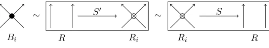
bimodules as objects inDb(A), the bounded derived category ofR-bimodules, we can give B i as a
mapping cone in two ways as shown in Figure 1.2. We have to pass toDb(A) because these maps, S and S0, are actually elements of Ext1(R, Ri) and Ext1(Ri, R) respectively. Here we label the
diagrams with their corresponding bimodules and use a box to denote a mapping cone. We will explain these diagrammatics in more detail in Chapters 3 and 4.
∼ S0 S
Bi R Ri
∼
Ri R
Figure 1.2: Bi as a mapping cone in Db(A).
These mapping cones correspond to two non-equivalent filtrations ofBi by standard bimodules, we will denote them byBi−andBi+respectively. The first hasRi as a submodule andRas a quotient module, and the second has R as a submodule and Ri as a quotient module. More importantly,
mapping cone presentations for Bott-Samelson bimodules as well. Letw=si1· · ·sikbe a non-reduced
word inSn, then a Bott-Samelson bimodule is a bimodule of the formBS(w) =Bi1 ⊗R· · · ⊗RBik.
Direct computation gives us the following proposition.
Proposition. BS(w) is quasi-isomorphic to an iterated mapping cone formed by tensoring together the mapping cone presentations of Bij for all j. The filtration induced on BS(w) from this iterated
mapping cone is equivalent to the tensor product filtration.
We can next prove the following relations for filtered Soergel bimodules in Db(A). We will use
the notation ∼F to mean filtered quasi-isomorphic.
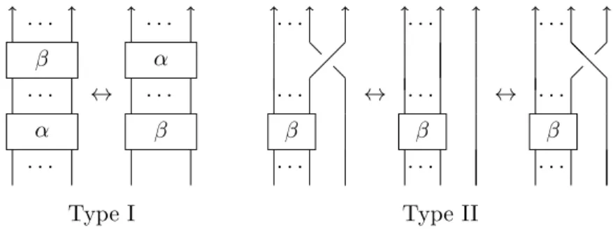
Proposition(Filtered Far Commutativity). Letε= +or−and letδ = +or−. ThenBiε⊗RBδj ∼F Bδ
j ⊗RBiε for |i−j| ≥2
Proposition (Filtered MOY II). Let ε= + or − and let δ= + or −. Then
Biε⊗RBδi ∼F Bic⊕bq2Bic0,
where c= + andc0=−if ε6=δ and c=−and c0 = + if ε=δ. Proposition (Filtered MOY III). Let δ1, δ2, δ3 ∈ {+,−}. Then
Bδ1
i ⊗RB δ2
i+1⊗RB
δ3
i ∼F
Cone(Y −→bq2B−δ1δ2δ3
i ) if δ2= + Cone(bq2B−δ1δ2δ3
i −→Y) if δ2=−
Here Y is the quotient bimodule (Bδ1
i ⊗RB δ2
i+1⊗RB
δ3
i )/B
−δ1δ2δ3
i .with the induced filtration.
In Chapter 5, we redefine the Rouquier complex in Kom(Db(A)) as shown in Figure 1.3 after
the appropriate grading shifts. Where χi and χo are the natural inclusion and projection maps associated to a mapping cone.
Given our new filtered Rouquier complex, we will prove the following results. Let G be the new Rouquier functor as above where G(αβ) = G(α)⊗RG(β) and G(1) = R. Let HF(β) denote the
= χ+ t b−1q−2 S
= t−1 S0 bq2 χ−
Figure 1.3: Redefinition of the Rouquier complex.
Theorem (Filtered Reidemeister II). The Reidemeister II isomorphism is a filtered homotopy equivalence. That is,
G(σiσi−1)'F G(1).
Theorem (Filtered Markov Moves). Let β∈ Bn. The following moves induce filtered isomorphisms
onHF(β).
I. Braid conjugation on β, that is replacing β =αα0 with α0α.
II. Positive or negative (de)stabilization on β, that is doing the replacement β7→βσ±1
n or vice
versa.
However, we can only conjecture invariance under Reidemeister III. We will also discuss this in more detail in Chapter 5.
Conjecture. Letβ andβ0be two braid representatives of a linkLwhich differ only by a Reidemeister
III isotopy (that is the relationσiσi+1σi =σi+1σiσi+1).ThenHF(β)is filtered isomorphic toHF(β0).
This conjecture and the preceding theorems immediately imply the following conjecture. Conjecture. LetL be a link and let β be a braid representative of L. Then HF(β)is a filtered link
invariant whose associated graded gives a quadruply-graded link homology theory.
Though we cannot prove invariance Reidemeister III, we can prove the following statement giving a bound on the possible error given by Reidemeister III.
Reidemeister III map from HF(β) to HF(β0) changes the filtration degree of x by at most 2 and fixes all other gradings.
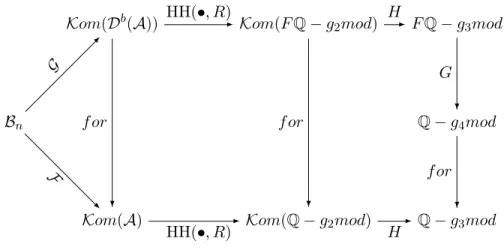
We now summarize the new process in contrast to the original process for HOMFLY-PT homology. Let Adenote the category of gradedR-bimodules. In the original process we apply the Rouquier functor, F, to the braid β, then we apply the Hochschild homology functor to get a complex of doubly-graded vector spaces, then we apply the homology functor to get HOMFLY-PT homology. In our new process we begin with a braid β, apply the filtered Rouquier functor G to get a complex of objects in Db(A). We then apply the Hochschild homology functor to get a complex
of doubly-graded filtered vector spaces. Finally we apply the homology functor to get a filtered triply-graded vector space, HF(β). We can then take the associated graded of this vector space to
get a quadruply-graded vector space. At every step we may apply a forgetful functorf or to return to the original process. The diagram in Figure 1.4 shows this process.
Kom(Db(A)) HH(•, R-) Kom(FQ−g2mod) H
- FQ−g3mod
Bn G
-Q−g4mod
G
?
Kom(A)
f or
?
HH(•, R-) F
-Kom(Q−g2mod)
f or
?
H- Q−g3mod f or
?
Figure 1.4: The process of computing H(β) and HF(β)
CHAPTER 2: The HOMFLY-PT and SL(N) Polynomials
In this chapter we begin defining elementary concepts in knot theory, and its relationship to braid groups. We then give two different constructions of both the HOMFLY-PT and SL(N) polynomials. Our first construction is the classical skein theoretic definition first given by Hoste, Ocneanu, Millet, Freyd, Lickorish, and Yetter [14] and also independently by Przytycki and Traczyk [34]. This definition arises by studying a representation of the braid groupBnon the Hecke Algebra Hn(q, a). Also we will discuss the construction given by Murakami, Ohtsuki, and Yamada using colored trivalent graphs [31]. This approach uses the Kazdahn-Lusztig basis ofHn(q, a) in defining the combinatorics of the trivalent graphs. The second construction is what is categorified in the subsequent link homology theories.
2.1 Preliminaries
Knot theory first appeared as a mathematical theory at the end of the 18th century. It was studied by A.T. Vandermonde, C.-F. Gauss, F. Klein and M. Dehn. A more systematic study of knots began at the end of the 19th century when mathematicans and physicists both began to tabulate knots. The preceding history and the following defintions are adapted from [28].
Definition 2.1.1. A link of mcomponents is a subset of S3, or of R3, that consists ofm disjoint,
smooth, simple closed curves. A link of one component is called a knot.
Intuitively we may envision a knot as a string which has been tangled up in some fashion and fused at the ends. With this perspective it makes sense to consider two knots the “same” if we may move around the strings without breaking them to make the two knots look identical. The following definition makes this idea mathematically precise.
Definition 2.1.2. Two links are called isotopic if one of them can be transformed to the other by a diffeomorphism h of S3, or of R3, such that h is homotopic to the identity in the class of
We will normally use the term link to mean both a link and its isotopy class. The main question in knot theory is the following: Given two links,L1 andL2, can we determine ifL1 is isotopic to
L2? The first step in attempting to solve these problems is to define a combinatorial method of describing links.
Definition 2.1.3. Alink diagram,D, of a link,L, is a projection onto a copy ofR2 embedded inside R3 that keeps the crossing information. In particular, the only singular points of the projection are
transverse double points and the preimages are distinguished by their z-coordinates, wherez is the coordinate transverse to the copy ofR2.
A simpler, yet still very difficult, question is can we determine if a link is isotopic to the unlink? The unlink is a link ofn components which has a link diagram consisting ofndisjoint copies of S1. A natural question can be asked. Is it possible to determine if two link diagrams D1 and D2 are diagrams for isotopic links? This question was answered positively by Reidemeister in 1926 [37] and by Alexander and Briggs in 1927 [2]
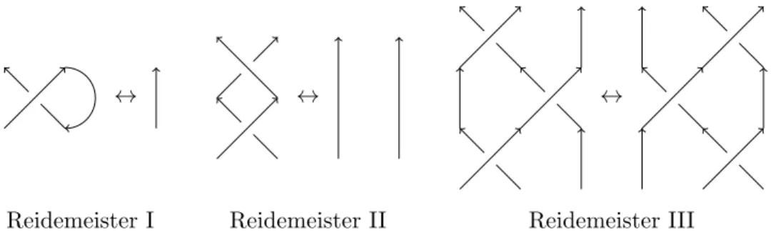
Theorem 2.1.4. Suppose thatD1 andD2 are two link diagrams. ThenD1andD2 represent isotopic links if they can be related by the a sequence of the following three moves, known as Reidemeister
moves.
I: Inserting or deleting a twist in either direction.
II: Move one strand completely on top of another.
III: Move a strand completely over or under another crossing.
These moves may be seen in Figure 2.1.
We may also study oriented links, that is a link where each component has a preferred direction which we will denote in a link diagram by the inclusion of arrows. If a link has ncomponents then there are 2n possible orientations. We will attempt to distinguish isotopy classes of links usinglink invariants. Roughly speaking, a link invariant is an object,P(L) we assoicate to a link such that the following is true: If two links, L1 and L2, are isotopic then their link invariants, P(L1) and
↔
Reidemeister I
↔
Reidemeister II
↔
Reidemeister III
Figure 2.1: Reidemeister Moves
2.2 Braids and Oriented Links
Next we discuss braids and their relationship to oriented links.
Definition 2.2.1. A braid of n strings, or briefly ann-braid, isn disjoint oriented arcs traversing
D2×[0,1] with strictly increasing t ∈ [0,1]. The arcs will join n standard fixed points in both
D2× {0}andD2× {1}. By convention we will assume that each arc’s orientation is in the direction of increasingt∈[0,1].
We can represent braids in diagrams in a similar manner to how we represent links. We will projectD2 onto an intervalI in such a way that the nstandard fixed points project onto distinct points. The we can easily see that two braids are isotopic if their diagrams differ by a sequence of Reidemeister moves of type II or III. Note that we may compose braids in the following manner. Suppose we have twon-braids β and β0, then we define the product braid β0β by juxteposing two braids and rescaling the t-coordinate as shown below in Figure 2.2.
σi i i+1
σi−1 i i+1
· · · · · · · · ·
· · ·
· · · · · · · · ·
· · ·
β
β0
β ∗ β0 =
Define the elementary n-braids σ1±1, ..., σn±−11 by the diagrams above in Figure 2.2. It is not hard to see thatσiσ−i 1 is isotopic to a braid with no crossings andσiσi+1σi is isotopic toσi+1σiσi+1using the Reidemeister moves. Therefore we may place a group structure on n-braids. We will associate to the braid with no crossings the identity element of the group.
Definition 2.2.2. The Artinn-braid group, which we denote by Bn, is the group generated by the elementary n-braids with the following presentation:
Bn=hσ1, ..., σn−1|σiσi+1σi =σi+1σiσi+1, σiσj =σjσi if|i−j| ≥2i.
We will use this group structure in the sequel when describing the HOMFLY-PT polynomial in terms of representations of Bn. Now we want to look at the relationship between braids and links.
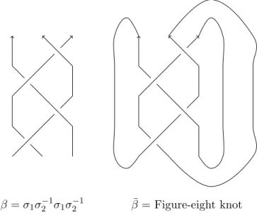
Note that if we take a braid diagram for a braid β and identify the endpoints in the manner shown in Figure 2.3, we receive an oriented link inS3. We will call this link theclosure ofβ and denote it by ¯β. The first question we may ask is if any link can be constructed in such a manner. The answer was given by Alexander in 1923.
β =σ1σ2−1σ1σ2−1 β¯= Figure-eight knot
Figure 2.3: A Braid and Its Closure as an Oriented Link
Theorem 2.2.3 (Alexander’s Theorem [1]). LetL be an oriented link. Then there exists a braid β
The next question we can ask is can we determine if two braids have isotopic closures. Markov in 1935 determined exactly when two braids give rise to isotopic links [30]. First we will define the two moves Markov introduced. These moves are pictured in Figure 2.4.
Definition 2.2.4. Let α, β∈ Bn. AType I Markov move, orconjugation, takes αβ toβα.
Definition 2.2.5. Letβ ∈ Bn. AType II Markov move, or(de)stabliazation, takesβ 7→βσn±1∈ Bn+1 (or vice versa).
Theorem 2.2.6 (Markov’s Theorem). Let β ∈ Bn andβ0∈ Bn0. β andβ0 have isotopic closures if and only if we may transform β to β0 by a sequence of braid isotopies and Markov moves.
· · ·
· · · · · ·
β
α
· · ·
· · · · · ·
α
β
↔
Type I
· · · · · ·
· · ·
β
· · · · · ·
· · ·
β
· · ·
· · ·
β
↔ ↔
Type II
Figure 2.4: Markov Moves
2.3 Hecke Algebras and the HOMFLY-PT Polynomial
Before we discuss the HOMFLY-PT polynomial we will discuss Hecke algebras. The goal of this section is to construct Hecke algebras, and to discuss special properties of these algebras. We will denote the Hecke algebra byHn(q, a) or simply Hn when q anda are understood. In particular we will discuss a representation ofBn on Hn.
Definition 2.3.1. The Hecke algebraHn(q, a) is theZ(q, a)-algebra generated by invertible elements Ti fori= 1, ..., n−1 in the following presentation.
Note that the relations for Hn look similar to the relations for the braid groupBn. This hints at
the possibility of a representation ofBn on Hn. We will define a representation ρ:Bn→Aut(Hn)
by setting ρ(σi) =Ti. Here we useTi to represent both the element inHn and the automorphism of
Hn which is multiplication byTi. We now want to define a trace on Hn.
Theorem 2.3.2 (Ocneanu, [14]). Fix z∈C. There exists a linear trace tr:Hn→C(q, a) uniquely
defined by the following axioms.
1. tr(xy) =tr(yx) 2. tr(1) = a−a
−1
q−q−1 3. tr(xTn) =ztr(x) Where x, y∈Hn.
We can normalize the generators Ti so that both possible types of the Markov move of type II
affect the trace in the same manner. We will omit the details of this normalization and only give the final result.
Theorem 2.3.3 (HOMFLY-PT polynomial, [14, 34]). Let β ∈ Bn and let L= ¯β. Then P(L) =
tr(ρ(β))is a link invariant in Z(q, a) satisfying the skein relation
aP(L+)−a−1P(L−) = (q−q−1)P(L0).
Here L+, L− and L0 are oriented links which are the same except in a neighborhood of a point where they are shown in Figure 2.5. We define P(Unknot) = a−a
−1
q−q−1.
L+ L− L0
Figure 2.5: Conway Triple
Now we will define theSL(N) polynomial. This polynomial can be obtained by studying the representation theory of Uq(sl(N)) (See [31] for example), but we will describe it here in terms of
Definition 2.3.4 (SL(N) polynomial). TheSL(N) polynomial is a function
Pn:{Oriented Links} →Z(q). It is defined by Pn(L) =P(L)|a=qn.
Remark. We can also obtain the Jones and Alexander polynomials from the HOMFLY-PT polynomial as well. The Jones polynomial is the SL(2) polynomial, P2, and the Alexander polynomial P0 is found by settinga= 1 andP0(Unknot) = 1.
2.4 MOY Construction of HOMFLY-PT and SL(N) polynomials
Finally we will discuss a construction of the HOMFLY-PT polynomial using polynomial invariants of certain graphs. We will only define what is needed to construct the HOMFLY-PT and SL(N) polynomials. Their construction was first given by Murakami, Ohtsuki and Yamada in 1998 for the
SL(N) polynomial in terms of trivalent graphs colored by positive integers [31]. This construction can be extended to the HOMFLY-PT polynomial as well. Our exposition here follows Rasmussen’s in [35].
First we define what we will call braid graphs. A braid graph is a braid in which all crossings are replaced with singular crossings, which we will mark as the vertex of the graph. An example is shown below in Figure 2.6. The MOY state model of the HOMFLY-PT polynomial resolves a braid into a formal sum of braid graphs with coefficients in Z(q, a) in the following manner. We
may resolve each crossing in two ways; we may remove a crossing entirely and replace it with two vertical arcs, or we may replace a crossing with a singular crossing. To each resolution we assign a weight µ∈Z. If we resolve the crossing into vertical arcs, we assign the resolution a weight of 0. If we resolve the crossing into a singular crossing, we assign a weight of 1 if the crossing was positive and -1 if the crossing was negative.
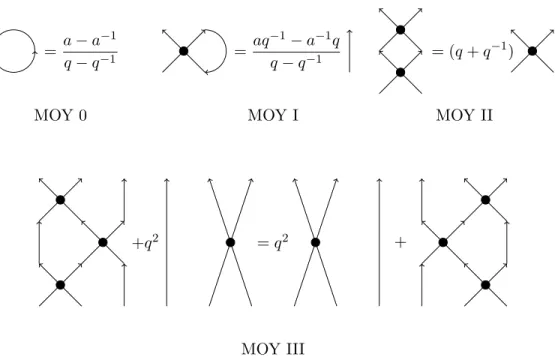
= a−a −1
q−q−1 =
aq−1−a−1q
q−q−1 = (q+q
−1)
MOY I
MOY 0 MOY II
+q2 =q2 +
MOY III
Figure 2.7: MOY Relations for Braid Graphs
Now let D be a link diagram in the form of a braid closure. A state of the diagram, σ, is a choice of resolution for each crossing in the link diagram. If a diagram hasncrossings then it will have 2n possible states. We define the weight of a state,µ(σ), to be sum of the weights of each resolution in the state. Also note that each stateσ gives rise a closure of a braid graph Dσ. In the paper by Murakami, Ohtsuki, and Yamada [31] it was shown that the unnormalized HOMFLY-PT polynomial can be expressed as a sum
P(L) = (aq−1)w(D)X
σ
(−q)µ(σ)P(Dσ).
Where P(Dσ) is defined by graph isotopy and the relations, which we will refer to as the MOY relations, in Figure 2.7. It can be shown that these relations are sufficient to compute the HOMFLY-PT polynomial.
These braid graphs give a graphical representation of the Kazdhan-Luzstig basis of Hn(q, a).
Hn(q, a) =hb1, ..., bn−1|bibj =bjbi for |i−j| ≥2,
b2i = (1 +q2)bi,
bibi+1bi+q2bi+1 =bi+1bibi+1+q2bii.
We can associate the braid graphs shown in Figure 2.8 to bi. If we define multiplication of
braid graphs by vertical concatenation as we did with braids, the MOY relations are exactly these relations for the Kazdhan-Lusztig basis.
· · · ·
bi i i+1
Figure 2.8: Kazdhan-Luzstig Basis represented by Braid Graphs
We may also write a MOY state model for the SL(N) polynomial as well. This is what was originally presented in [31]. In this presentation we only need perform the substitution a=qn to recieve the SL(N) polynomial.
Remark. It is not necessary for the computation ofP(L) and Pn(L) by MOY graphs to take Lto
be a braid closure. In the original paper by Murakami, Ohtsuki, and Yamada, they computePn(L)
from an arbitrary link diagram. However in the sequel, it is strictly necessary for us to consider L
CHAPTER 3: HOMFLY-PT Homology
In 2004, Khovanov and Rozansky announced a categorification of theSL(N) polynomial using
Z2−graded matrix factorizations of potentials being sums and differences ofxni+1 [23]. In 2005 they
also announced a generalization of this which gave a triply-graded cohomology theory categorifying the HOMFLY-PT polynomial using Z2−graded matrix factorizations of potentials being sums and differences ofa(xi−xj) [24]. In 2006, Khovanov made a connection between this theory and Rouquier’s braid group action on the objects of a certain homotopy category using Soergel bimodules [21, 38]. In this chapter we will discuss Soergel bimodules, Hochschild homology, and how these can be used to define Khovanov and Rozansky’s HOMFLY-PT homology. Our approach will mainly follow [21].
3.1 Soergel Bimodules
Let R=Q[x1, ...xn] and letRi =Q[x1, ..., xi−1, xi+xi+1, xixi+1, xi+2, ..., xn]. The ringRi is the
ring of polynomials which are symmetric inxi andxi+1, or equivalently the polynomials fixed by the action of the permutation which interchanges iand i+ 1. It is clear thatR is a free Ri-module of rank 2. We will also make the rings R andRi graded by setting degq(xi) = 2, and call this grading the “q-grading” or the “internal grading”. Define the R-bimodule Bi=R⊗RiR. This is a graded
bimodule inheriting the grading from R. Bi is free of rank 2 as both a left R-module and a right R-module.
Definition 3.1.1. LetR=Q[x1, ..., xn]. Thecategory of Soergel bimodules,S, is the full subcategory of graded R-bimodules generated by tensor products of Bi, their direct summands, and grading shifts.
Kazhdan-Lusztig basis ofHn(q, a) mentioned in the previous chapter. The following proposition will state
exactly what is meant by this statement.
Proposition 3.1.2 ([39]). Let qn denote the grading shift functor that raises the q-grading of a bimodule byn. Then there are isomorphisms of graded R-bimodules
Bi⊗RBj ∼=Bj ⊗Bi , if |i−j| ≥1, Bi⊗RBi ∼=Bi⊕q2Bi,
(Bi⊗RBi+1⊗RBi)⊕q2Bi+1 =∼q2Bi⊕(Bi+1⊗RBi⊗RBi+1).
The first two isomorphisms follow directly from definitions. The third isomorphism is non-trivial. LetRi,i+1 be the subring of R fixed by any permutation permutingi,i+ 1 andi+ 2. Now define
Bi,i+1=R⊗Ri,i+1R. Then Soergel in [39] shows there areR-bimodule isomorphisms
Bi⊗RBi+1⊗RBi∼=Bi,i+1⊕q2Bi,
Bi+1⊗RBi⊗RBi+1∼=Bi,i+1⊕q2Bi+1.
The last isomorphism in the proposition follows immediately. We will call the relations in Proposition 3.1.2 categorified MOY relations for reasons which will become clear in what follows. We want to also want to describe the indecomposable Soergel bimodules.
Theorem 3.1.3 (Soergel [41]). For any fully reduced word w=si1· · ·sik ∈Sn, there exists up to
isomorphism a unique indecomposable Soergel bimoduleBw which occurs as a direct summand of
BS(w) = Bi1 ⊗R· · · ⊗RBik, but does not occur as a summand of BS(w
0) for any w0 < w with respect to the Bruhat order. Reduced words w∈Sn give a full description of indecomposable Soergel
bimodules up to grading shifts.
Example 3.1.4. Let we letn= 3, then the indecomposable Soergel bimodules are
where Bs1s2 =B1⊗RB2, Bs2s1 =B2⊗RB1,and Bs1s2s1 =Bi,i+1.
We want to now introduce a system of diagrammatics to help us visualize computations with Soergel bimodules. Our diagrammatics will follow almost exactly the conventions of Khovanov and Rozansky [21, 22]. All Soergel bimodules will be represented by an upward oriented graph with each incoming and outgoing strand labelled with a variable. First we will denoteR=Q[x1, ..., xn]
by a diagram with nvertical lines oriented upward. We will denoteBi using the same diagram that we used for the Kazdhan-Lusztig basis elementbi.
· · ·
R x1
y1 yn
xn x1
y1
xn
yn
Bi
· · · ·
yi yi+1 yi yi+2
xi xi+1 x1 xi xi+2
y1
xn
yn
Bi,i+1 · · · ·
Figure 3.1: Diagrams forR,Bi andBi,i+1
We will also denote Bi,i+1 by the diagram shown in Figure 3.1. If we wish to take the tensor product of Soergel bimodules, sayM ⊗RN, we will denote this by taking the diagram for M and gluing it on top of the diagram for N. We will leave marks on the diagram to denote where the gluing occurs. Once we introduce standard bimodules and virtual crossings we will discuss these markings in more detail. Finally we may place diagrams adjacently horizontally as well. If we place the diagrams forM and N in such a manner this will correspond to M⊗QN.
· · · · · ·
· · ·
N N
M⊗RN
· · · · · ·
M
· · · · · ·
M
M⊗QN
3.2 Rouquier’s Braid Group Action
Let R= Q[x1, ..., xn]. Let S denote the category of Soergel bimodules. Then let Kom(S) be
the homotopy category of Soergel bimodules, that is the category of chain complexes of Soergel bimodules up to homotopy equivalence. In [38], Rouquier proposed a categorification of Bn
us-ing chain complexes of Soergel bimodules inKom(S). In this section we will describe his construction.
Definition 3.2.1. The category of n-braids, which we will denote by Bn, is the category whose
objects aren-braids and whose morphisms are braid cobordisms.
First we will define two morphisms χ+:R →Bi and χ−:Bi →R. R has a single generator, 1,
inq-degree 0. Therefore we will define
χ+(1) =xi⊗1−1⊗xi+1.
Also Bi has a single generator, 1⊗1, in q-degree 0. We can see this by considering Bi as a
quotient ofR⊗R, which we will do whenever convenient. We will define
χ−(1⊗1) = 1.
Note that degq(χ+) = 2 and degq(χ−) = 0. Now we will define Rouquier’s braid group action on Kom(S). Define F :Bn→ Kom(S) by
F(1) = 0 - R - 0,
F(σi) = 0 - R
χ+
- tq−2Bi - 0,
F(σ−i 1) = 0 - t−1Bi χ−
- R - 0,
F(ββ0) =F(β)⊗RF(β0) for β, β0∈Bn.
Here we use a nonstandard notation for homological degree. We will usetk to denote that the
Theorem 3.2.2 (Rouquier [38]). Let F be defined as above, then 1. F(σiσi−1)' F(1).
2. F(σiσi+1σi)' F(σi+1σiσi+1).
Here 'denotes homotopy equivalence inKom(S).
We will discuss an outline of the proof of this theorem. When we are trying to prove the analogous statements for the filtered case, the outline of the proof will be similar. First we give a lemma which will help to simplify chain complexes. A proof of this lemma may be found in [4]. Lemma 3.2.1 (Gaussian Elimination). Consider the complex,
A (
•
α)
- B⊕C
ϕ λ µ ν
- D⊕E
(•ε)
- F,
in any additive category where ϕ:B →D is an isomorphism and all other maps are arbitrary up to the condition that d2 = 0. Then there exists a homotopy equivalence
A (
•
α)
- B⊕C
ϕ λ
µ ν
- D⊕E
(•ε)
- F A (1) ? (1) 6
(α)
- C
( 0 1 )
?
−ϕ−1λ
1
6
(ν−µϕ−1ε)
- E
(−µϕ−11 )
?
(01)
6
(ε)
- F
(1)
?
(1)
6
First we will give an outline of the proof for (1) of Theorem 3.2.2. By definition
F(σiσ−i 1) =F(σi)⊗RF(σi−1),
R
F(σiσi−1) = t−1Bi χ−
-⊕ tq−2Bi χ
+
-q−2Bi⊗RBi χ−
-χ
+
-Proposition 3.1.2 tells us thatBi⊗RBi∼=Bi⊕q2Bi. We can apply this isomorphism toF(σiσi−1)
to get the following complex.
R
F(σiσi−1) ' t−1Bi χ−
-⊕ tq−2Bi χ
+
-q−2Bi⊕Bi π1
-i2
-Here i2 is the inclusion map into the second direct summand and π1 is the projection map onto the first direct summand. Therefore by Gaussian Elimination we see that
F(σiσ−i 1)'(0 - R - 0) =F(1).
Now we will give an outline of the proof for (2) in Theorem 3.2.2. The basic idea of this proof is to show thatF(σiσi+1σi) and F(σi+1σiσi+1) are both homotopy equivalent to a complex which is fixed by the permutation switchingx1 andx3. The permutation corresponds to reflecting a braid across a vertical axis. We can write F(σiσi+1σi) as a cube. We will abbreviate the terms in the
R - tq−2Bi
F(σiσi+1σi)= tq−2Bi
-t2q−4BiBi
-tq−2Bi+1
?
- t2q−4Bi+1Bi ?
t2q−4BiBi+1
?
-t3q−6BiBi+1Bi ?
-In the above complex, the maps are omitted. By Proposition 3.1.2, we know thatBi⊗RBi∼= Bi⊕q2Bi and Bi⊗RBi+1⊗RBi ∼=Bi,i+1⊕q2Bi. Therefore by applying these isomorphisms to F(σiσi+1σi) we get a new complex.
R - tq−2Bi
F(σiσi+1σi)' tq−2Bi
-t2q−4Bi⊕t2q−2Bi
(∗ 1)
-tq−2Bi+1
?
- t2q−4Bi+1Bi ?
t2q−4BiBi+1
?
-t3q−6Bi,i+1⊕t3q−4Bi
(∗ ∗1∗)
?
may apply Gaussian Elimination to this complex to get the below complex.
tq−2Bi - t2q−4BiBi+1
F(σiσi+1σi)' R
-t3q−6Bi,i+1
-tq−2Bi+1
-t2q−4Bi+1Bi
-The above complex can be shown to be “symmetric”, that is the complex is fixed under the permutation ofx1 andx3. It can be easily shown that F(σi+1σiσi+1) is homotopy equivalent to the same complex but withx3 andx1 permuted. This completes the outline of the proof of Theorem 3.2.2.
Remark. F : Bn → Kom(S) is actually a functor. It was shown by Elias and Krasner that this
construction was functorial with respect to braid cobordisms [12]. More precisely, if S andS0 are equivalent braid cobordisms fromβ toβ0, thenF(S) andF(S0) are homotopy equivalent maps from F(β) to F(β0).
= χi
= t−1 χo
tq−2
Figure 3.3: Diagrammatic form of F(σ1) and F(σ−11)
3.3 Koszul Resolutions
In this section we will define Koszul complexes and describe when these complexes are free resolutions of R-modules, and then we will use this to define the Hochschild homology of Soergel bimodules. Finally we will introduce diagrammatics for Hochschild homology and explain our choice of diagrammatics. Our exposition here follows [21, 22, 45].
Suppose for this discussion that R is a commutative ring with unity. The ringR=Q[x1, ..., xn] will be the primary example we will keep in mind. Let p∈R, then let K(p) be the chain complex
K(p) = 0 - R
p
- R - 0
with terms concentrated in homological degree 0 and 1. IfR is a graded ring with degq(p) =k, then we shift the copy of R is homological degree 1 by qk to make multiplication by pa degree 0 map. That is,
K(p) = 0 - qkR p
- R - 0.
Definition 3.3.1. Let p = (p1, ..., pn) be a sequence of elements in R. We define the Koszul
complex,K(p), as the tensor product complex
K(p) =K(p1)⊗R· · · ⊗RK(pn).
Proposition 3.3.2. Suppose p is a regular sequence in R. That is, pi is not a zero divisor in
R/(p1, ..., pi−1)R for alli. Then
Hk(K(p)) =
0 if k6= 0
R/pR if k= 0
A proof of this proposition can be found in Weibel [45].
particular if A is an R-module then,
TorRk(R/pR, A) =Hk(K(p)⊗RA)
ExtkR(R/pR, A) =Hk(Hom(K(p), A))
Before moving on we want to introduce an alternate notation for Koszul complexes. Suppose p= (p1, ..., pn) is a sequence of elements inR, then will also present K(p) as a column vector,
K(p) =
p1 p2 .. . pn
From this point forward we will use this presentation whenever it convenient. We will also use brackets instead of parentheses for the vectors to minimize possible confusion. An advantage of this presentation is that we can see change of basis transformations as row operations.
Proposition 3.3.4. Let p= (p1, ..., pn) be a sequence in aR. Then there exists an invertible chain map Φki→j such that
Φki→j :
pi pj → pi
kpi+pj
and all other rows are fixed.
Proof. The map Φki→j is defined as
R pi
pj
- R⊕R
(−pjpi)
- R
R
1
? pi
kpi+pj
- R⊕R
1 0
k1
?
(−kpi−pjpi)
- R
1
?
3.4 Hochschild Homology of Soergel Bimodules
We will begin by defining Hochschild homology, and then look at the Hochschild homology of Soergel bimodules. Our definitions and basic results about Hochschild homology follow [45]. Hochschild homology is a homology theory used to study properties of algebras and their bimodules. Let kbe a field, letR be ak-algebra, and setRe=R⊗kR. Note that if M is aRe-module, then it is also aR-bimodule. The basic example we will keep in mind isk=Qand R=Q[x1, ..., xn]. Definition 3.4.1. Let M be a R-bimodule, the we define the Hochschild homology of R with coefficients in M to be
HHk(M, R) = TorR
e
k (M, R).
Also we define
HH(M, R) =M
k≥0
HHk(M, R).
IfR is understood, then we may abbreviate HH(M) = HH(M, R). Remark. We may also defineHochschild cohomology by setting
HHk(M, R) = ExtkRe(M, R).
However we will only be using Hochschild homology in the sequel. Proposition 3.4.2. Let k=Q and let R=Q[x1, ..., xn]. Then
HHk(R, R)∼= Λk(Rn).
Proof. First we want to carefully describe R as an R-bimodule. Recall that any R-bimodule can also be thought of as an R⊗Q R-module. From basic commutative algebra we know that
R⊗QR∼=Q[x1, ..., xn, y1, ..., yn], so then clearlyR∼= (R⊗QR)/I whereI = (x1−y1, ..., xn−yn).
The sequence p= (x1−y1, ...xn−yn) can easily be shown to be a regular sequence. Therefore by Corollary 3.3.3,K(p) is a freeRe-module resolution of R. That is,
K(p) =
k O
Therefore the functor • ⊗ReR identifies the variables xi and yi so that
K(p)⊗Re R=
k O
i=1
(R−→0 R).
From this we see that HHk(M, R) = TorR
e
k (R, R) =R(
n
k)∼= Λk(Rn).
Finally we will mention some useful basic and “trace-like” properties of Hochschild homology. Theorem 3.4.3. Letkbe a field,Ran k-algebra andM, N beRe-modules. The following properties
hold for Hochschild homology.
1. HHk(•, R) and HH(•, R) are additive functors.
2. HHk(M ⊕N, R)∼=HHk(M, R)⊕HHk(N, R).
3. HHk(M ⊗RN, R)=∼HHk(N⊗RM, R).
4. Let 0−→M1 −→ M2 −→ M3 −→0 be a short exact sequence of Re-modules, then there exists a long exact sequence
· · ·−→∂ HHk(M1, R)−→HHk(M2, R)−→HHk(M3, R)
∂
−→HHk−1(M1, R)−→ · · ·
Proof. (1) and (2) follow from the properties of the TorRe
k (•, R) functor. Property (3) follows from
looking at projective resolutions ofM⊗RN and ofN⊗RM. Finally (4) is an exercise in [45]. Now we return to discussing Soergel bimodules. We want to be able to compute the Hochschild homology HH(M, R) for any Soergel bimoduleM. To do so we need to know more about the general structure of these bimodules.
Proposition 3.4.4. Let M be a Soergel bimodule. Then as a Re-module,
M ∼=Re/I1⊕ · · · ⊕Re/Im.
Proof. By Theorem 3.1.3, any Soergel bimoduleM can be expressed as a sum of indecomposable Soergel bimodules,
M ∼=
n M
i=1 qkiBw
i,
wherewi ∈Sn. In [21], Khovanov shows that every indecomposable Soergel bimodule can be written in the formRe/I where I is an ideal generated by a regular sequence.
By Proposition 3.4.4 we know that the Koszul complex for any Soergel bimodule is a free
Re-module resolution of M. Therefore we can use this to compute the Hochschild homology. Here we introduce a grading convention for Hochschild homology. We will use the notation akpto denote that the Hochschild degree or a-degree, dega(p), of p is being shifted up by k. In particular if
p ∈ HHj(M, R) then akp ∈HHj+k(akM, R). By convention we will say that dega(p) = 0 for all p∈R. We will also use the same notation ak to denote that a term lies in homological degree k
in a Koszul complex. This notation is consistent as these terms become Hochschild chains after applying the left derived tensor product.
Example 3.4.5. Let R = Q[x1, x2] and M = B1 = R⊗R1 R. By studying the left and right
actions byRonB1 we see thatB1∼=Q[x1, x2, y1, y2]/(x1+x2−y1−y2, x1x2−y1y2) as Re-modules. p= (x1+x2−y1−y2, x1x2−y1y2) is a regular sequence, so then the Koszul complex K(p) is a free resolution. Recall that Soergel bimodules are also graded with degq(xi) = 2. The same will be
true for yi as it represents the right action byxi. Therefore,
K(p) = (aq4Re x−−−−−−−1x2−y1y→2 Re)⊗Re(aq2Re x1+x2
−y1−y2
−−−−−−−−−→Re).
Once again, the functor• ⊗ReR identifies the variables xi and yi so that
K(p) = (aq4R−→0 R)⊗R(aq2R −→0 R).
This implies that HH(B1, R) =a2q6R⊕aq4R⊕aq2R⊕R.We can also revisit the calculation for HH(R, R), while keeping track of the gradings, to show that
Therefore, HH(R, R) and HH(B1, R) arenotisomorphic as graded objects though they are isomorphic as non-graded objects.
We now introduce some basic diagrammatics for Hochschild homology to coincide with what has already been introduced for Soergel bimodules. SetR=Q[x1, ..., xn], and letM be an R-bimodule.
The we will denote HH(M, R) by closing the strands of the graph as if we were closing a braid. This is shown in Figure 3.4. This diagram hints at the fact that Hochschild homology may be right analog to taking the trace for computing the HOMFLY-PT polynomial.
· · · · · ·
M
Figure 3.4: Diagram for HH(M, R)
Also recall that from Theorem 3.4.3, we know that HHk(M ⊗RN, R)= HH∼ k(N ⊗RM, R).We
can visualize this isomorphism by sliding the box forM around the closed strands and moving it to underneath the box forN. This process is shown in Figure 3.5.
· · ·
N
· · · · · ·
M
· · ·
M
· · · · · ·
N
· · · · · ·
M
· · · · · ·
N
↔ ↔
3.5 HOMFLY-PT Homology
Before defining HOMFLY-PT homology of a link L, we will introduce shifts to the Rouquier complexes and the Hochschild homology functor. When we are going through the proof of the Markov moves it will become apparent why these shifts are needed. The idea of using fractional shifts was first introduced by Hao Wu in [47]. We will follow that approach here.
Let β ∈Bn be a braid representative for a linkL. Let s =t−1/2qa1/2. We define the shifted
Rouquier complex by Fe(σi) = sF(σi), and F(e σi−1) = s−1F(σi−1). Direct computation shows
that these shifts do not violate the isomorphisms proved in Theorem 3.2.2. Also as before we set
e
F(ββ0) = F(e β)⊗RF(e β0) for β, β0 ∈ Bn. We also define a shifted Hochschild homology functor g
HH(•, R) =sna−nHH(•, R).
Now we describe how to compute H(L). We first apply the functor Fe to a braid representative
of L,β, to receive a chain complex
· · · d- Fej−1(β)
d
- Fej(β) d
- · · · .
We then apply our shifted Hochschild homology functor gHH(•, R) toF(e β) to get a new chain
complex,
· · · HH(g d-) gHH(Fej−1(β), R)
g
HH(d)
- HH(g Fej(β), R) g
HH(d)
- · · · .
Define H(β) =H(gHH(F(e β), R)).
Theorem 3.5.1. (Khovanov, Rozansky [24]) Let L be a link and β∈Bn be a braid representative for L. Then H(L) =H(β) is a triply-graded vector space which is a link invariant categorifying the HOMFLY-PT polynomial P(L).
categorifying the HOMFLY-PT polynomial P(L). We can expressH(L) as
H(L) = M
j∈Z,i,k∈1 2Z
tiqjakQd(i,j,k).
Then by Theorem 3.5.1,
P(L) = X
j∈Z,i,k∈1 2Z
d(i, j, k)(−1)i+kqjak.
We have to do a change of variables to get back to our original conventions for the HOMFLY-PT polynomial. The conventions used for the gradings forH(L) give
P(Unknot) = 1 +aq 2 1−q2 .
If we letα=p−aq2, and multiply byqa−1 then we have
P(Unknot) = a−a −1
q−q−1
as in our original conventions.
We know from Theorem 3.2.2 that H(L) is preserved by Reidemeister II and III. It remains to show that the Markov moves hold as well. the Markov move of type I holds by part (3) of Theorem 3.4.3. It remains to check Markov moves of type II. We will only discuss the proof of the case of positive stabilization, that is βσn being replaced by β.
Define theclosing functor C`i(•) =•
L
⊗Q[xi,yi]Q[xi, yi]. We can think of this as a “partial” left
derived tensor product, which corresponds to closing only the ith strand of our braid diagram. To prove positive stabilization it will suffice to prove that fC`2(F(e σ1)) ∼= F(1), wheree fC`i(•) =
t−1/2qa−1/2C`i(•) is the shifted closing functor and 1 denotes the trivial braid in one strand. In our diagrammatics this corresponds to the positive version of Reidemeister I (See Figure 2.1).
We first consider the Koszul resolutions of R and B1
R=
x1−y1
x2−y2
B1 =
x1+x2−y1−y2
x1x2−y1y2
By applying Φ12→1 to the Koszul complex forR and replacing y1 with x1+x2−y2 we may rewrite the Koszul complexes as
R=
x1+x2−y1−y2
x2−y2
B1 =
x1+x2−y1−y2 (x2−y2)(x1−y2)
.
Seta=x2−y2, b=x1−y2,and w=x1+x2−y1−y2. Khovanov and Rozansky prove in [24] that we may now writeF(σi) as the complex
w a
Id⊗ψ - tq−2
w ab ,
where ψ:K(a)→K(ab) is the map
K(a) = aq2R a - R
K(ab) =taq2R
1
? ab
- tq−2R b
?
Now we apply C`2 to this complex, this identifies x2 and y2. Let R0 = Q[x1, x2, y1], then C`2(F(σ1)) is
K(a) = aq2R0 0 - R0
K(ab) =taq2R0
1
? 0
- tq−2R0. x1−x2
?
This complex splits into two direct summands. The first summand,
is contractible by Gaussian elimination. So we are left with a short complex
R0 x1−x-2 tq−2R0.
If we letR00=Q[x1, y1], we can rewrite this complex as
R0
0
x1−x2
- tq−2R00⊕tq−2(x1−x2)R00.
CHAPTER 4: Virtual Crossings and Filtrations
Virtual crossings were first considered as a tool in link homology by Khovanov and Rozansky in [22]; they used virtual crossings to construct a conjectural link homology theory categorifying the KauffmanSO(2n) polynomial. In an appendix of this paper, they also discussed how the concept of virtual crossings could be introduced to HOMFLY-PT homology as well. Also Thiel showed that Rouquier’s braid group action on the category of Soergel bimodules could be extended to a virtual braid group action on a slightly larger category of bimodules which includes not only indecomposable Soergel bimodules, but also their irreducible submodules [42].
In this chapter we shall introduce the basics of virtual braids and links. Then we will define what are known as “standard bimodules” and explain how they relate to Soergel bimodules and virtual crossings. We will then show how Soergel bimodules can be filtered by standard bimodules and how these filtrations can be expressed in terms of mapping cones in the proper category.
4.1 Virtual Braids and Links
Virtual links were first introduced by Kauffman in 1996 [18]. They were first defined as equivalence classes of Gauss codes. Gauss codes encode the crossing data of links, up to certain relations which generalize the Reidemeister moves in this setting. We will discuss virtual links from the viewpoint of virtual link diagrams and also speak about the topological interpretation of virtual links as given by Kuperberg [27].
Definition 4.1.1. A virtual link diagram is an oriented planar 4-regular graph endowed with the following structure: each vertex is either considered an over crossing, an under crossing, or is marked by what we will call avirtual crossing. If a crossing is not virtual then we call itclassical and if a virtual link diagram has no virtual crossing we call it aclassical link diagram.
Figure 4.1: Virtual crossing and virtual trefoil knot
Definition 4.1.2. We call two virtual link diagrams equivalent if there exists a sequence of generalized Reidemeister moves that transforms one diagram into the other. The generalized Reidemeister moves are the following (see Figure 4.2):
1. Classical Reidemeister moves, that is the moves of Figure 2.1.
2. Virtual versions of the classical Reidemeister moves. We will call these virtual Reidemeister I, II, and III, or briefly VRI, VRII, and VRIII.
3. The semivirtual Reidemeister move, or briefly SVR.
It should be noted that the move in Figure 4.3, called the forbidden move, is not allowed. Definition 4.1.3. A virtual link is an equivalence class of virtual link diagrams modulo the generalized Reidemeister moves.
Proposition 4.1.4 ([19]). If two classical links are related by generalized Reidemeister moves, then they are isotopic in the classical sense. Also if a link only has virtual crossings then it is equivalent
to an unlink.
Kuperberg proposed a topological interpretation of virtual links in 2003 involving embeddings of links on genus g surfaces, Sg, which have been slightly thickened, which we will denote by Σg =Sg×(−ε, ε) [27]. When we project onto R2×(−ε, ε), actual crossings in Σg induce classical
=
VRI
=
VRII
=
VRIII
=
SVR
Figure 4.2: Generalized Reidemeister Moves
6=
Figure 4.3: Forbidden Move
Let g(L) denote the number of virtual crossings of a virtual link diagram L. Then we have an embedding ψ: s(L) →Σg(L), where s(L) is a disjoint union of circles equal to the number of components of L.
Definition 4.1.5. We say that two such embeddings are stably equivalent if one can be obtained from the other from isotopy in the thickened surfaces, homeomorphisms of surfaces, or the addition or subtraction of handles which are not incident to the images of the curves.
Theorem 4.1.6 (Kuperberg [27]). Two virtual link diagrams generate equivalent virtual links if and only if their corresponding surface embeddings are stably equivalent.
Definition 4.1.7. The virtual n-braid group, which we denote by VBn, is the group generated by the elementary n-braidsσi and the elementary virtual braidsvi, with the following presentation:
VBn=hσ1, ..., σn−1, v1, ..., vn−1|σiσj =σjσi if|i−j| ≥2, σiσi+1σi =σi+1σiσi+1
vivj =vjvi if|i−j| ≥2, vivi+1vi =vi+1vivi+1
v2i = 1
viσi+1vi =vi+1σivi+1
σivj =vjσi if|i−j| ≥2i
The first two relations are the classical braiding relations for Bn. The next three relations describe how virtual crossings interact. In particular the relationvivi+1vi=vi+1vivi+1 represents virtual Reidemeister III and v2i = 1 represents virtual Reidemeister II. The last two relations represent how classical and virtual braids interact, in particular the relation viσi+1vi =vi+1σivi+1 represents the semivirtual Reidemeister move.
σi i i+1
σi−1 i i+1
vi i i+1
Figure 4.4: Elementary virtual braids
Remark 4.1.1. Inside of the virtual braid group VBn we have two important subgroups. The
subgroup generated by the elements vi is isomorphic to the symmetric group Sn and the subgroup
generated by the elementsσi is the classical braid groupBn.
for virtual links. Let β∈ VBn. We define the closure of a virtual braid, ¯β, as we did before with the closure of a braid.
Theorem 4.1.8 (Kauffman [18]). Let L be a virtual link. Then there exists a virtual braid β such thatβ¯is equivalent to L.
Also similar to the case for classical links, we can tell when two virtual braids close to the same link. We will now define a virtual analog of the Markov moves. The Type I and Type II Markov moves (Definitions 2.2.4 and 2.2.5) remain the same for virtual braids and we will not redefine those moves. We will introduce two new Markov moves, both of which are pictured in Figure 4.6. Definition 4.1.9. Let α, β ∈ VBn. A Type IIIa Markov move, or a right virtual exchange move takes ασnβσ−n1 toαvnβvn
Definition 4.1.10. Let α, β ∈ VBn. Let α0 and β0 be the images of the embedding of VBn to
VBn+1 on the last n strands. A Type IIIb Markov move, or a left virtual exchange move takes
α0σ1β0σ1−1 toα0v1β0v1
Theorem 4.1.11 (Kamada [17]). Let β ∈ VBn and β0 ∈ VBn0. β and β0 have equivalent closures if and only if we may transform β to β0 by a sequence of relations in the virtual braid groups and
Markov moves of type I, II, IIIa, and IIIb.
α
β ↔
α
β
Type IIIa · · ·
· · ·
· · · · · ·
α0
β0
· · · · · ·
α0
β0
↔
Type IIIb · · · · · ·
Figure 4.5: Markov Moves of Type IIIa and IIIb
4.2 Standard Bimodules
the “right” categorification of virtual crossings in the category of graded bimodules. For most of this discussion we will follow [41].
Let R=Q[x1, ..., xn], Sn be thenth symmetric group, and let w∈Sn. Sn acts on R as before taking xi to xw(i). Define the standard bimodule Rw as an R-module isomorphic to R as a left
R-module with rightR-actionf ·x=w(x)f. These bimodules are also graded with degq(xi) = 2. We can also describeRw as aR⊗QR-module,
Rw ∼=Q[x1, ..., xn, y1, ..., yn]/(x1−yw(1), ..., xn−yw(n)).
It is easily shown that pw = (x1−yw(1), ..., xn−yw(n)) is a regular sequence, so thatK(pw) is a
Koszul resolution forRw. If w0 ∈Sn also then we can considerRw⊗RR0w. Rw⊗RR0w is isomorphic
to R as a left R-module. If f ⊗g ∈ Rw⊗RR0w then by definition (f ⊗g)·x = f ⊗(g·x) = f⊗w0(x)g= (f·w0(x))⊗g= (ww0(x)f)⊗g=ww0(x)(f⊗g). ThereforeRw⊗RR0w∼=Rww0.
Proposition 4.2.1. Let w, w0 ∈Sn, then Hom(Rw, Rw)=∼R andHom(Rw, Rw0) = 0 if w6=w0. Proof. Recall that for a commutative ring S,HomS(S/I, S/J) ∼= (J :I)/J where (J :I) ={s∈
S|sJ⊂I}. If we consider Rw= (R⊗QR)/(pw) andRw0 = (R⊗
QR)/(pw0), then the result follows immediately.
Let ST be the full subcategory of graded R-bimodules generated byRw for allw∈Sn up to direct sums and grading shifts.
Theorem 4.2.2. ST is a categorification of the group ringZ[q±1][Sn].
Proof. K0(ST) is a ring with, [M ⊗RN] = [M][N], since ST is a monoidal category. We want to
define a mapφ:K0(ST)→Z[q±1][Sn]. We will set φ(qk[Rw]) =qkw.BecauseRw⊗RR0w∼=Rww0, Rw⊗RRw−1 ∼=ReandRsi⊗RRsi+1⊗RRsi ∼=Rsi+1⊗RRsi⊗RRsi+1. Thereforeφis a ring morphism.
It remains to show that φis invertible, butψ(w) = [Rw] is an inverse for φas desired.
Now we will give the justification for the terminology “virtual crossings” in relation to standard bimodules.
F(1) = 0 - R - 0,
F(vi) = 0 - Rs
i - 0,
F(σi) = 0 - R
χ+
- tq−2Bi - 0,
F(σ−i 1) = 0 - t−1Bi χ−
- R - 0,
F(ββ0) =F(β)⊗RF(β0) for β, β0 ∈Bn.
Then ifβ andβ0 are words representing the same element ofVBn, then F(β) is homotopy equivalent
to F(β0).
Therefore, inA, the bimodulesRsi represent the action of virtual crossings in the virtual braid
group. With this in mind we will now define diagrammatics for the bimodulesRw. First we associate toRsi the diagram for the elementary virtual crossingvi. To tensor productsRw⊗RRw0 we associate
concatenation of diagrams as before.
xi
x1 xi+1 xn yi
y1 yi+1 yn
Ri
Figure 4.6: Standard bimodule as virtual crossing
4.3 Soergel Bimodules and Filtrations
We now want to introduce how Soergel bimodules and standard bimodules interact. First we consider the Soergel bimoduleBi. For now we restrict ourselves to a certain subclass of Soergel bimodules called Bott-Samelson bimodules.
Definition 4.3.1. Let w=si1· · ·sik be a (not necessarily reduced) word in Sn. A Bott-Samelson
BS(w) =Bi1 ⊗R· · · ⊗RBik
Remark 4.3.1. Note that two words, w and w0, being equivalent in Sn does not imply that
BS(w)∼=BS(w0). For example we know from the categorified MOY relations that
BS(s1s1) =Bi⊗RBi =∼Bi⊕q2BiR=BS(1).
We will now set Ri=Rsi for brevity. There exists a short exact sequence
0 - q2R
xi+1⊗1−1⊗xi
- Bi 1 - Ri - 0. (4.1)
Therefore, R is a submodule of Bi and Ri ∼= Bi/R. We can also encode this information in
the form of a filtration. By convention, we will consider only finite decreasing filtrations, that is filtrations of the form
F(M) : 0 =Fi(M)⊂Fi−1(M)⊂ · · · ⊂Fi−k(M) =M.
Also recall the associated graded module of a filtered module is defined as GF(M) =L
iGFi (M)
where GF
i (M) =Fi(M)/Fi+1(M).
In the case of the short exact sequence (4.1), we may define the positive filtration of Bi, F1+(Bi) =q2R and F0+(Bi) =Bi. The associated graded of this filtration
G+(Bi) =GF+(Bi) =G+1(Bi)⊕G+0(Bi).
In this caseG+1(Bi) =q2R andG+0(Bi) =Ri. We can also consider another short exact sequence
0 - q2Ri xi
⊗1−1⊗xi
- Bi 1 - R - 0 (4.2)
q2Ri and F0−(Bi) =Bi. The associated graded of this filtration is
G−(Bi) =GF−(Bi) =G−1(Bi)⊕G−0(Bi).
In this caseG−1(Bi) =q2Ri andG−0(Bi) =R.
We can also define filtrations on any Bott-Samelson bimodule in a similar manner. Recall that ifM and N are filtered bimodules, then M⊗RN is also a filtered bimodule with
Fp(M⊗RN) = X
i+j=p
Fi(M)⊗RFj(N).
Note that this sum is normally not a direct sum, but rather the sum P
i+j=pIm(ιi,j) with ιi,j : Fi(M)⊗RFj(N)→M⊗RN being the inclusion map.
Let w=si1· · ·sik ∈Sn and let ∆ ={δ1, ..., δk} be a sequence of pluses and minuses. Then we
can define the filtration F∆ on BS(w) by
Fp∆(BS(w)) = X
j1+···+jk=p
(Fδ1
i1(Bs1)⊗R· · · ⊗RF
δk
ik(Bsk))
Example 4.3.2. Let w=s2s1 ∈S3 and let ∆ ={+,−}. Then we can define F∆(BS(w)) by the following.
F2∆(BS(w)) =F1+(B1)⊗RF1−(B2) =q2R⊗Rq2R2∼=q4R2
F1∆(BS(w)) =F1+(B1)⊗RF0−(B2) +F0+(B1)⊗RF1−(B2) =q2R⊗RB2+B1⊗Rq2R2∼=q2B2+q2B1⊗RR2
F0∆(BS(w)) =F0+(B1)⊗RF0−(B2) =B1⊗RB2
Direct computation and carefully looking at the sum of inclusions for F1∆(BS(w)) tells us that
G∆2(BS(w)) =R2, G∆1(BS(w)) =R⊕Rw, G∆0(BS(w)) =R1.
Theorem 4.3.3 (Soergel [41]). Let Bw be the indecomposable Soergel bimodule labelled by w∈Sn.
Then there exists a unique filtration Fstd(Bw), called the standard filtration, such that
Gstdi (Bw) = M
x≤w,`(x)=i
q2iRx.
Soergel used these filtrations to prove that Bx categorifies the Kazdahn-Lusztig basis of Hn and
to give a proof of the Kazdahn-Luzstig positivity conjecture forHn.
4.4 Some Homological Algebra
In this section we will discuss how we may convert filtrations of bimodules into iterated mapping cones in a derived category. When we have filtrations which have length greater than 2, it becomes more natural to replace iterated mapping cones with convolutions of twisted complexes. We will introduce twisted complexes and their convolutions and give some basic results. Finally we will explore how a special type of homotopy equivalence, deformation retracts, interact with twisted complexes and their convolutions.
Suppose we have a R-bimoduleM and a filtration onM of length two. That is
0 =F2(M)⊂F1(M)⊂F0(M) =M.
Then we can write a short exact sequence
0 - F1(M) - F0(M) - G0(M) - 0
Let Adenote the category of graded R-bimodules. Let us now considerM as a filtered object inDb(A), the bounded derived category of A. Then the short exact sequence above implies that
M ∼Cone(G0(M)−→s G1(M)).
When we are using diagrammatics, instead of writing Cone(s) we will draw a box around a short complex as shown in Figure 4.7
ConeX−→f Y= X f Y
Figure 4.7: Alternate notation for mapping cones
We want to find a similar way to describe longer filtrations of bimodules in the bounded derived category. Via an inductive argument using short exact sequences,
0 - Fp(M) - Fp−1(M) - Gp(M) - 0,
we see that we can express the filtration as an iterated mapping cone on the associated graded modules
G0(M) G1(M) G2(M) · · · Gk−1(M) Gk(M)
.
However, iterated mapping cones can be burdensome to work with. We will introduce an alternative way of dealing with these objects known as twisted complexes.
Definition 4.4.1. A twisted complex overDb(A) is a collection
{Xi, fij :Xj →Xi}i∈Z≥0
consisting of finitely many objectsXi ∈ Db(A), X0 6= 0 and mapsfij ∈Hom∗(Xj, Xi) of homological
degree i−j−1 which satisfy the following relations.
• fij = 0 if j≥i.
• ∂fij :=dXifij + (−1)
i−j+1fijdX
j =
X