Simulations of the tidal interaction and mass transfer of a star
in an eccentric orbit around an intermediate-mass black hole:
the case of HLX-1
Edwin van der Helm,
1‹Simon Portegies Zwart
1and Onno Pols
21Leiden Observatory, Leiden University, PO Box 9513, NL-2300 RA, Leiden, the Netherlands
2Department of Astrophysics/IMAPP, Radboud Universiteit Nijmegen, PO Box 9010, NL-6500 GL Nijmegen, the Netherlands
Accepted 2015 October 3. Received 2015 September 8; in original form 2014 December 5
A B S T R A C T
The X-ray source HLX-1 near the spiral galaxy ESO 243-49 is currently the best intermediate-mass black hole candidate. It has a peak bolometric luminosity of 1042erg s−1, which implies
a mass inflow rate of∼10−4 M yr−1, but the origin of this mass is unknown. It has been proposed that there is a star on an eccentric orbit around the black hole which transfers mass at pericentre. To investigate the orbital evolution of this system, we perform stellar evolution simulations usingMESAand smoothed particle hydrodynamics simulations of a stellar orbit
around an intermediate-mass black hole usingFI. We run and couple these simulations using
theAMUSEframework. We find that mass is lost through both the first and second Lagrange
points and that there is a delay of up to 10 d between the pericentre passage and the peak mass-loss event. The orbital evolution time-scales we find in our simulations are larger than what is predicted by analytical models, but these models fall within the errors of our results. Despite the fast orbital evolution, we are unable to reproduce the observed change in outburst period. We conclude that the change in the stellar orbit, with the system parameters investigated here, is unable to account for all observed features of HLX-1.
Key words: hydrodynamics – methods: numerical – binaries: close – stars: kinematics and dy-namics – X-rays: binaries – X-rays: individual (HLX-1).
1 I N T R O D U C T I O N
The X-ray source HLX-1 has an estimated peak bolometric isotropic luminosity of ∼1042 erg s−1 (Farrell et al. 2009). With redshift
measurements of the optical counterpart, Wiersema et al. (2010) and Soria, Hau & Pakull (2013) argue that HLX-1 coincides with the spiral galaxy ESO 243-49, but it does not coincide with its nucleus. The source transits in a few days from the low/hard X-ray state to the high/soft X-X-ray state during which the count rate increases by an order of magnitude (Godet et al. 2009; Servillat et al.2011). During this transition, Webb et al. (2012) have detected radio flares. The X-ray spectrum has been fitted using black hole accretion disc spectral models (Davis et al.2011; Godet et al.2012; Straub et al.2014). These arguments have been used to claim that HLX-1 hosts a black hole with a mass between∼104and ∼105
M (Webb et al. 2012). This mass range is consistent with an intermediate-mass black hole (IMBH; e.g. Miller & Colbert2004). The luminosity of HLX-1 follows a fast rise and exponential decay pattern with a period of approximately 370 d (Lasota et al.
E-mail:[email protected]
2011). Various scenarios have been investigated to explain this ob-served X-ray light curve, which postulate a star on an eccentric orbit around an IMBH. This star would experience Roche lobe overflow at pericentre, transferring mass to the black hole. The transferred mass would then form an accretion disc and the mass accreting on to the black hole would emit the X-rays (Shakura & Sunyaev1973). The observed 370 d periodicity in the X-rays can then be interpreted as the orbital period of this companion star around the black hole.
To date, five complete outbursts of HLX-1 have been observed with the Swift X-ray telescope (Godet et al. 2012, 2014). An overview of the time evolution of the shape of the outbursts is presented by Miller, Farrell & Maccarone (2014). The peak X-ray luminosity decreases with each outburst and the decay time also decreases, which means that the integrated energy per outburst de-creases. In the proposed mass transfer models, these observations would correspond to a stable semimajor axes (a) and a decrease of the mass transfer rate ( ˙M).
In 2013, the expected outburst occurred more than a month later than predicted from the previously observed outburst period (Godet et al.2014). The outburst after that occurred in 2015 with an even larger delay (Kong, Soria & Farrell2015). To understand the first delay, Godet et al. (2014) performed smoothed particle
namics (SPH) simulations of the tidal capture of a star (e.g. Baum-gardt et al.2006) on to a highly eccentric (e>0.9998) orbit around a black hole. In their scenario, the pericentre passage induces os-cillations in the star and the phase of these osos-cillations at the next pericentre passage affect the tidal forces. As this phase is essen-tially random, the tidal forces can induce stochastic variations in the orbital period (Ivanov & Papaloizou2004). These stochastic variations can explain the observed delay under the assumption that viscous processes do not damp the oscillations between pericentre passages. In this tidal capture model, the star will only orbit the black hole for∼102yr before it is expelled again.
An alternative scenario to explain the observed X-ray light curve has been proposed by Miller et al. (2014). They postulate an en-counter between the IMBH and a high-mass giant star between 5 and 15 yr ago. In this encounter, the envelope of the giant star would have been stripped by tidal interaction with the black hole. The core of the giant would have remained on an eccentric orbit around the black hole. This core would have a low-mass hydrogen envelope which it loses through a strong stellar wind. At every peri-centre passage this wind feeds the accretion disc and from that point onward, this scenario follows the same arguments as the scenario proposed by Lasota et al. (2011). This second scenario predicts that the stripped envelope material will be accreted on to the black hole resulting in a stable bright X-ray signal within 10–100 years. From the current observations, Miller et al. (2014) have not been able to exclude either scenario for HLX-1.
The observations of HLX-1 indicate that the black hole has an accretion disc which has been studied by fitting disc models to the observed spectra. The disc is cool (Davis et al.2011) and thin (Godet et al.2012) and has an outer radius between 15 and 150 R(Soria 2013). It has not been possible to directly constrain the nature or the orbit of the stellar companion of HLX-1 from the observations, but the periodicity of the X-ray signal is interpreted as periodic mass transfer at pericentre, which would imply that the orbit is not circular. By assuming that the outer radius of the accretion disc corresponds to the pericentre distance of the stellar orbit, So-ria (2013) derive an eccentricity ofe≈ 0.95, with a lower limit ofe≈0.9.
The direct mass transfer model has been proposed (Lasota et al. 2011) to explain the current observations. If we assume that the direct mass transfer model is correct, then the question remains: What is the origin and long-term orbital evolution of the stellar companion? In this paper, we combine SPH simulations and stellar evolution models to study the orbital evolution of the star during mass transfer. We then compare the results of these simulations with analytical predictions of this orbital evolution. Using the orbital evolution from our simulations, we will attempt to constrain the origin and long term orbital evolution of the stellar companion of HLX-1.
2 S E T T I N G T H E S C E N E
There is a general agreement between independent measure-ments of the black hole mass (MBH) using Eddington scaling
(MBH > 9·103M, Servillat et al.2011), accretion disc
mod-els (MBH≈103−5M, Davis et al.2011; Godet et al.2012; Straub
et al.2014) and the detection of ballistic jets (MBH≈104−5M,
Webb et al.2012). Here, we will adoptMBH=10 000 Mbased
on the assumption that at the peak of the outbursts, the IMBH lumi-nosity is near the Eddington lumilumi-nosity. Following the direct mass transfer model, we assume that the orbital period is equal to the observed periodicity of the outbursts (370 d). Using the equations
for a Keplerian orbit, the semimajor axis can be calculated from the orbital period and total mass of the system (a=21.7 au), where the total mass is essentiallyMBH. The initial parameters used in this
work are summarized in Tables2and3.
For the outer radius of the accretion disc (rdisc) we use the largest
value from observations, sordisc= 150 R (Soria2013). If the
pericentre distance (rp) corresponds to the outer radius of the
ac-cretion disc, thene≈ 0.95 (Soria2013). The outer radius of the accretion disc does not necessarily correspond torp, other factors
in the complex physics of accretion discs can limit the outer ra-dius. We therefore investigate a lower value ofe=0.7, as well as e=0.95. The stellar angular velocity (∗) is not constrained by the observations, we therefore perform simulations with 0, 0.5 and 1 times the orbital angular velocity at pericentre (orb,p).
2.1 The donor star
To determine the stellar radius (R∗), we start with the volume equiv-alent Roche radius for a star in an eccentric binary (RRoche). If
R∗<RRoche, no mass transfer occurs but tidal interaction will affect
the shape of the donor as well as the orbit. IfR∗RRochemass will
flow from the donor to the black hole, which is the case of interest in this study. We therefore adoptR∗≈RRoche in our calculations.
Determining the value ofRRocheas a function of the mass ratio and
orbital parameters requires numerical evaluation of the gravitational potential. In this paper, we use fitting formulas forRRoche(Eggleton
1983; Sepinsky, Willems & Kalogera2007a). We perform a series of simulations using 0.8<R∗/RRoche<1.2 to investigate the effect
of different mass-loss rates on the orbital evolution.
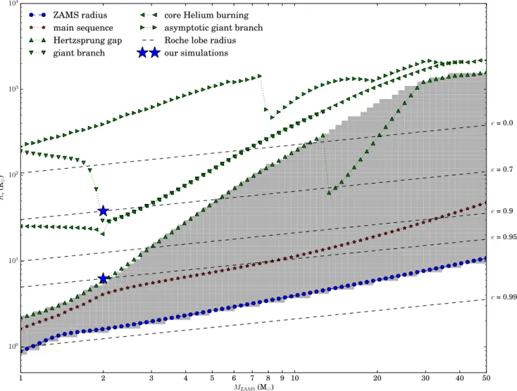
The stage of stellar evolution that the star is in whenR∗≈RRoche
depends on the zero-age main-sequence mass (MZAMS) of the star
and the orbital parameters. In Fig. 1, we compare R∗ at differ-ent stellar evolution stages withRRochefor various values ofeand
MZAMS with metallicity Z = 0.02. The star can be on the main
sequence whenR∗=RRoche if it has a high eccentricity and large
mass (e0.95 andMZAMS8 M). The large blue stars in Fig.1
correspond to the orbital and stellar parameters used in this work. The star we use in our simulations is a giant with a convective envelope.
The stellar mass determines the stellar lifetime; therefore the possible mass range of the stellar companion depends on the age of the stellar population near HLX-1. Observations favour a young (∼20 Myr) stellar population, but an additional older population cannot be excluded (Farrell et al.2014). Because the companion star can originate from either population, there is only a limited observational constraint on the massM∗of the companion star. We adoptMZAMS=2 M.
2.2 Orbital evolution processes
Before and during mass transfer, the star orbiting the IMBH is sub-ject to tidal dissipation. The effects of tidal dissipation on the orbit of a star with a convective envelope are commonly described by the equilibrium tide model (Zahn1977; Hut1981; Rasio et al.1996; Eggleton, Kiseleva & Hut1998). As a result of the tidal dissipation, the orbit gradually becomes circular (e=0) and the star will evolve towards corotation. Corotation is defined as the state where the stel-lar angustel-lar velocity equals the orbital angustel-lar velocity (∗=orb).
Figure 1. The maximum radii of stars during various stages in the stellar evolution as a function of initial mass usingSEBA(Portegies Zwart & Verbunt2012) with metallicityZ=0.02. The ZAMS radii represent the start of the main sequence. The black dashed lines correspond to the Roche lobe radius of the stellar companion of HLX-1 for each mass. Each line corresponds to a given eccentricity, shown on the right-hand side of the figure. Stars in the grey shaded region have a radiation dominated stellar envelope while all other stars have a convection dominated envelope. The large blue stars represent the parameters used in our simulations. For a 2 Mstar, mass transfer occurs during the asymptotic giant branch ife=0.7, or at the start of the giant branch ife=0.95.
the orbital angular velocity at pericentre (∗>0.799orb,p) (Hut
1981). The rate of change of the orbital and stellar parameters de-pends on the stellar radius as ˙a∝R8
∗, ˙e∝R∗8and ˙∗∝R∗6. The
tidal dissipation is stronger when the star has a convective envelope than when it has a radiative envelope, in which case the equilibrium tide model is inadequate.
The main uncertainty in the equilibrium tide model is the tidal damping time-scale (T), which is usually estimated in combination with the apsidal motion constant (k) because the rates of change in the tidal evolution equations scale withk/T. The constantkis a measure of the central condensation of the star, where lowerk corresponds to a higher central condensation (e.g. Hut1981). A theoretical estimate ofk/Tas a function of the stellar parameters has been calculated by Rasio et al. (1996). However, comparisons with observations indicate thatk/Tshould be larger (e.g. Meibom & Mathieu2005; Belczynski et al.2008). Using the equations of Hut (1981) and Rasio et al. (1996) and the observed parameters of HLX-1 (withR∗=RRoche), we find that, due to tidal dissipation,
∗changes on a time-scale of∼102–4yr,achanges on a time-scale
of∼106yr andechanges on a time-scale of∼107–8yr.
If a star in a binary loses mass, the orbit changes due to the change in the mass and angular momentum of the star. The lost mass can be transferred from the star to the other object, and part of the mass can be ejected from the system. The evolution of the orbit due to mass transfer whene>0 has been studied analytically (Sepinsky et al.2007b, 2009). They calculate the change in the semimajor axisaand the eccentricityeas a function of ˙M∗. They assume that the mass is lost or transferred instantaneously during the pericentre passage, and that all mass leaves the star through the first Lagrangian point L1 of the eccentric orbit. Using these
equations and the observed parameters of HLX-1, we find thata changes on a time-scale of∼104–5 yr ande changes on a
time-scale of∼105–6yr due to mass transfer. Mass transfer in eccentric
binary systems has also been studied using SPH (Regos, Bailey & Mardling2005; Church et al.2009; Lajoie & Sills2011) but they did not investigate the effect on the orbit.
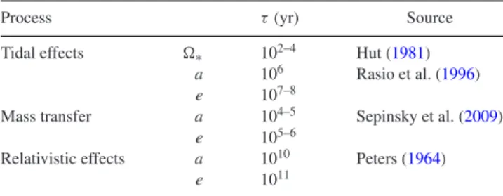
Table 1. An overview of the time-scales (τ) of the orbital and stellar pro-cesses in HLX-1. For a parameterX, the time-scaleτX is defined here as
|X/X˙|. The second column contains the affected parameter and the third column contains the literature source for the value or analytical formula. Where applicable, system parameters from Section 2 have been used.
Process τ(yr) Source
Tidal effects ∗ 102–4 Hut (1981)
a 106 Rasio et al. (1996)
e 107–8
Mass transfer a 104–5 Sepinsky et al. (2009)
e 105–6
Relativistic effects a 1010 Peters (1964)
e 1011
not change through mass transfer or tidal interactions. They argue that this assumption is valid when the stellar specific orbital energy (E, orb∝MBH/a) is larger than the stellar specific binding energy
(E, bind∝M∗/R∗). This would imply thatais constant, which is not
the case for our system (see Table1). Furthermore, even ifawhere constant, changes inecould still affect the mass transfer.
Relativistic effects can affect the orbit of a star near a black hole. The first relativistic correction that causes a change inaand eis the emission of gravitational waves. The magnitude of this effect can be calculated using the equation from Peters (1964), which results in an orbital evolution time-scale of∼1010–11yr. This
is considerably longer than the orbital evolution caused by other effects and therefore we conclude that relativistic effects can be ignored in this work.
In Table1, we summarize the time-scales of the evolutionary processes discussed in this section. The change in∗through tidal effects is faster than the change in the other orbital and stellar parameters. The evolution ofaandeappears to be dominated by mass transfer rather than tidal effects, but this may not be entirely correct due to the uncertainty ink/T. We therefore take both tidal effects and mass transfer into account in our simulations.
3 M E T H O D S
We simulate the evolution of HLX-1 in two steps. The first step spans∼109yr, in which we simulate the stellar evolution up to the
present day. The second step spans∼10 yr, in which we simulate the hydrodynamical evolution of the system in detail.
In the first step, we evolve a single star in isolation until it has a radius comparable to the Roche radius in the chosen initial orbit. In principle, we cannot assume that the star has evolved in isolation because the formation history of HLX-1 is unknown. However, if the star evolved on an orbit similar to the current orbit, thenR∗<RRoche
and the influence of the black hole is negligible during this part of the evolution. If the star was captured into the present orbit, it would have evolved far from the black hole, and we can also assume it evolved in isolation.
We convert the one-dimensional stellar structure model to a three-dimensional gas model. We place this star in a Keplerian orbit around the black hole usingMBHand orbital parameters from
Sec-tion 2. This complete system is then used as the initial condiSec-tion for the second and most important part of our simulations.
In the second step, we simulate the detailed three-dimensional gas- and gravitational dynamics of the system. The mass transfer resulting from the gravitational interaction is measured and we calculate the orbital mechanics of all gas. We then calculate the secular change in the orbit of all gas that is bound to the star. The
time for which we simulate this step is comparable to the time for which HLX-1 has been observed. We have also performed a number of longer simulations to investigate the change in∗through tidal interaction.
3.1 Numeric implementation
We use theAMUSE1 framework (Pelupessy et al.2013; Portegies
Zwart et al.2013; van Elteren, Pelupessy & Portegies Zwart2014) to perform all simulations in this work. For the evolution of a single isolated star, we useMESA(Paxton et al.2011) as it is implemented
in AMUSE.MESAis a one-dimensional Henyey code which can be
used to perform stellar evolution calculations by assuming spherical symmetry and hydrostatic equilibrium. For the three-dimensional simulations of gas-dynamics we useFI (Pelupessy2005) as it is
implemented in AMUSE. FI is an SPH (Monaghan1992) code in
which the gas is represented by discrete particles.
To create the three-dimensional gas model of the star, we take the radial density, temperature and mean molecular mass profiles from theMESAmodel and generate a set of SPH particles. This is done
using theAMUSEroutinestar_to_sph.py(de Vries, Portegies Zwart & Figueira2014). Accurately simulating high-density regions requires small time-steps in SPH simulations, simulating the core of the star therefore requires more CPU time than the envelope. However, to study mass transfer and tidal interactions, we mainly have to resolve the outer parts of the star and not the core. We therefore replace the stellar core with a single mass point and prevent the star from collapsing by adding Plummer softening to the core particle. The softening length depends on the mass of the core particle and the original density profile (de Vries et al.2014).
The IMBH is represented by a single point mass in the SPH code, which is also a sink particle (Bate, Bonnell & Price1995). At every step in the simulation, any SPH particle within a radiusrsink from
the black hole is accreted, which is implemented in thesink.py routine inAMUSE. We do not resolve the accretion disc but we set
the radius of the black hole sink particle equal to the radius of the accretion disc (rsink=rdisc).
3.2 Relaxation
Part of the SPH method is that the kernel function induces a non-physical force that prevents the SPH particles from approaching each other arbitrarily close (e.g. Price2012). Particles can start close together because the initial spatial distribution of SPH particles is chosen randomly and therefore this non-physical force can add energy and cause the star to expand, which is not physical. To prevent this from happening, the gas has to be relaxed in the correct gravitational potential before we start the simulation. Because the gravitational potential is not static in an eccentric orbit, we perform this relaxation in multiple steps.
In the first step, the particle distribution is brought to dynamical equilibrium in the fixed gravitational potential at apocentre in orbit around the black hole. For this step, we use the relaxation method described in section 3.3 of de Vries et al. (2014). We evolve the SPH system by a single timestep and subtract the bulk motion of the star to preserve the centre-of-mass position and velocity. Then, we decrease the change in velocity by multiplying it with a factor fthat increases linearly from 0 to 1 over 400 d (approximately one orbit).
In the second step, the star is evolved in a circular orbit with a semimajor axis (relaxation distance) arel = 10 au. We choose
this value because the star is close to the black hole but not close enough for mass transfer to occur. After one orbit, the relaxed star is returned to the apocentre position of the original orbit.
3.3 Orbital parameter determination
To calculate the (change in) orbital parameters, we need the mass, position and velocity of the black hole and the star. For the black hole, we know the position and velocity because it is a single particle in our simulation. For the star, we determine which SPH particles are bound to the stellar core particle and to each other, and then compute the total mass and the centre of mass position and velocity of these particles.
To determine the bound particles, we calculate the specific total energy (ES) from the internal (EU), kinetic (EK) and potential (EP)
energy of each particle. The internal energy is calculated within the SPH code. The kinetic and potential energy of each particle are calculated from the mass (Mc), position (Xc) and velocity (Vc) of
the stellar core, and the position (Xg) and velocity (Vg) of the gas
particle.
ES=EU+EK−EP (1)
EK=
1 2
Vg−Vc
2
(2)
EP= G∗M
c
Xg−Xc
(3)
Here, Gis the gravitational constant. We consider a gas particle bound to the stellar core whenES<0.
This set does not include all bound particles yet, as we have not taken the gravitational binding energy between gas particles into account. We therefore replaceMc, XcandVcwith the total mass,
the centre of mass and the centre of mass velocity of the stellar core plus the known bound particles and recalculateES. This procedure
is repeated until no more particles are added in the next iteration. In the calculations for a Keplerian orbit it is assumed that the black hole and the star are point particles. This assumption is valid while the radius of the star is far smaller than the orbital separation. Because this assumption is not valid near pericentre, the computed orbital parameters are not constant throughout the orbit. We cal-culate all orbital evolution trends from the orbital parameters as measured at apocentre.
3.4 Stellar radius determination
Both the rate of tidal evolution of the binary system and the rate of mass transfer are very sensitive to the radius of the donor star. In order to make a comparison between the simulations and analytical prescriptions, we need to have a good estimate of the stellar radius from the simulations. In SPH simulations, it is hard to acquire such an estimate because the star is represented by a set of discrete particles. We have experimented with various methods to measure the radius, such as using the outermost bound particle or using the mean distance from the centre of mass of thenoutermost SPH particles. However, we found that these methods are far too sensitive to a small number of barely bound SPH particles in the outer regions of the star. We solve this problem by introducing a density cut-off (ρcut) and we measure the stellar radius at this density.
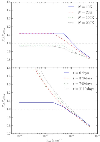
In Fig. 2we present the measured stellar radius for different values ofρcut. The radius at a fixed density is smaller for higher
Figure 2. The radius of the SPH realization of the star calculated with different values of the density cut-off (ρcut) for different resolutions (top panel) and different times in the simulation (bottom panel). The radius of theMESAmodel is shown with dashed black line, we find good agreement with theMESAmodel forρcut=5×10⁻⁷g cm−3. Ifρcutis smaller than this value, the measured radius at later times in the simulation is very large and completely dominated by a few SPH particles that are only barely bound to the star.
resolution and larger at a later time in the simulation. When we adopt a density cut-off of 5×10⁻⁷g cm−3, the SPH radius determination
is consistent (within 5 per cent) with the results from the stellar evolution code for the resolution used in this work.
3.5 Model parameters
Using a computer simulation to approximate a physical process introduces a number of assumptions that are generally characterized by free parameters. Here, we summarize the assumptions used in this work and test the effect of varying these free parameters on our results.
For the stellar evolution simulations, we assume a metallicity Z= 0.02, but the actual metallicity of the star is unknown. The stellar wind mass-loss follows the Reimers mass-loss model with an efficiencyηR=0.5 (Reimers1975). We do not include convective
overshooting in the stellar evolution simulations.
Figure 3. The change in the stellar angular velocity while the star is far away from the black hole (the distance is greater than the semimajor axis) as a function of resolution. d∗/dtshould be 0 this far from the black hole and we see that forN>10 000 a largerNdoes not result in a smaller d/dt.
The resolution of the simulation depends on the number of SPH particles (N). The mass of individual SPH particles is inversely proportional to their number, in the sense that more particles result in a higher resolution, but this comes at the expense of more computer time. We search for a balance between cost and resolution using convergence tests. We base our convergence test on∗ because this parameter is important for the tidal interactions discussed in Section 2.2.
For the main convergence test, we require that the angular velocity of the donor star (∗) is stable when the star does not interact with the black hole. Characterizing the stellar rotation rate by a single value∗is not always possible because different parts of the star can have different rotational velocities. However, we have found that the star in our simulations generally rotates as a rigid body when it is far away from the black hole, so we can take∗to be the average ofof all the SPH particles that represent the star. For this reason, we measure the rotation rate of the star in the binary when the distance between the black hole and the star is larger than the semi-major axis. For simulations where the star is initially not rotating,∗increases at every pericentre passage. In between pericentre passages, the rotation of the star should remain constant, but this turns out to depend on the resolution of the simulation. By performing several simulations with various resolutions we find that forN10 000, the erroneous change in∗does not depend onN(Fig.3). We conclude that the solution is converged and we useN=20 000.
At the resolution we have chosen, we still have a slight mismatch in the outermost density profile of the SPH realization compared to the underlying stellar evolution model (see Fig.4). This resolution therefore also does not result in a converged stellar radius compared to the stellar evolution model on which the initial realization was based (see Fig.3). Using a resolution that is high enough to ensure that the outermost density profile and the stellar radius are converged is not computationally feasible at this time. Instead, we take this limitation into account when interpreting our results. In Fig.4, we also see that gas near the core particle has a higher density than the gas in the underlying stellar evolution model. Because the effects studied in this paper are dominated by the behaviour of the outer layers of the star, we do not expect this discrepancy to affect our results.
An artificial viscosity (αandβ, see Monaghan1992) is required in SPH to model discontinuities such as shocks. The dimensionless
Figure 4. The radial density profile of theMESAmodel compared to the density of the SPH particles that represent it for different values ofN. The core 1 Mof the star is not included because it is not represented by SPH particles. It can be seen that models with more SPH particles have a lower density in the outermost layers of the star.
parameters can be chosen betweenα=β=0 (no artificial viscosity) andα=1;β=2 (artificial viscosity proportional to the resolution length). For simulations with strong shocks, an adaptive artificial viscosity can be used to correctly model instabilities (e.g. Morris & Monaghan1997). We do not expect strong shocks in our simulations so a fixed artificial viscosity is sufficient and we adoptα=0.5;
β=1.0 as these are the optimal values for most problems (Lombardi et al.1999). The value ofαcan influence the effectivek/Tin our simulations, and therefore we also perform simulations withα=0.1 andα=0.01 (andβ=2α) to quantify this effect.
As described in Section 3.1, we replace the core of the star with a single core particle with massMc. There are two practical constraints
that affect the value ofMc. IfMcis too large, the SPH particles that
represent the star cannot reproduce the stellar density profile. IfMc
is too small, the simulation will take a long time to run while the resolution at the surface of the star is not affected. We have created stellar models with a number of values ofMcand have found that
Mc=0.5MZAMSprovides a good balance between these constraints.
4 R E S U LT S
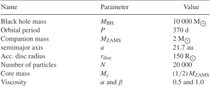
We have performed 20 simulations with different initial conditions to investigate the orbital evolution of HLX-1. In Table2, we present
Table 2. The initial parameters that we did not vary between the main sim-ulations used in this work. The initial parameters that we did vary between simulations can be found in Table3.
Name Parameter Value
Black hole mass MBH 10 000 M
Orbital period P 370 d
Companion mass MZAMS 2 M
semimajor axis a 21.7 au
Acc. disc radius rdisc 150 R
Number of particles N 20 000
Core mass Mc (1/2)MZAMS
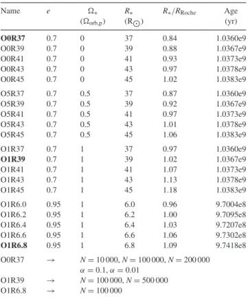
Table 3. The 20 main simulations used in this work and the initial param-eters that were varied between them. For the three simulations in bold font, we also performed eight additional test simulations varyingNandα(below table).
Name e ∗ R∗ R∗/RRoche Age
(orb,p) (R) (yr)
O0R37 0.7 0 37 0.84 1.0360e9
O0R39 0.7 0 39 0.88 1.0367e9
O0R41 0.7 0 41 0.93 1.0373e9
O0R43 0.7 0 43 0.97 1.0378e9
O0R45 0.7 0 45 1.02 1.0383e9
O5R37 0.7 0.5 37 0.87 1.0360e9
O5R39 0.7 0.5 39 0.92 1.0367e9
O5R41 0.7 0.5 41 0.97 1.0373e9
O5R43 0.7 0.5 43 1.01 1.0378e9
O5R45 0.7 0.5 45 1.06 1.0383e9
O1R37 0.7 1 37 0.97 1.0360e9
O1R39 0.7 1 39 1.02 1.0367e9
O1R41 0.7 1 41 1.07 1.0373e9
O1R43 0.7 1 43 1.13 1.0378e9
O1R45 0.7 1 45 1.18 1.0383e9
O1R6.0 0.95 1 6.0 0.96 9.7004e8
O1R6.2 0.95 1 6.2 1.00 9.7095e8
O1R6.4 0.95 1 6.4 1.03 9.7207e8
O1R6.6 0.95 1 6.6 1.06 9.7302e8
O1R6.8 0.95 1 6.8 1.09 9.7418e8
O0R37 → N=10 000,N=100 000,N=200 000 α=0.1,α=0.01
O1R39 → N=100 000,N=500 000
O1R6.8 → N=100 000
the initial conditions that we did not vary in the 20 main simula-tions. In Table3, we present the initial conditions that we did vary between the 20 main simulations. We used eight test simulations to investigate the effect of different values ofNandα. The 20 main simulations are divided into four sets with different orbital param-eters eand ∗. For each of these four sets, we have performed five simulations with different values ofR∗. We have performed the O1R39 simulation withN=500 000 twice to investigate an unex-pected effect of the numerical error in the angular momentum (see Section 4.3). The age at which the star reaches the desired radius is also included in Table3.
4.1 Tidal dissipation
Before investigating the combined effects of tidal dissipation and mass-loss on the stellar orbit, we isolate the effect of tidal dissipa-tion. We choose a simulation in which the stellar radiusR∗<RRoche
(model O0R37, see Table3) so that mass-loss is negligible. In the absence of mass-loss, the change in the orbital parameters is domi-nated by the effects of tidal dissipation.
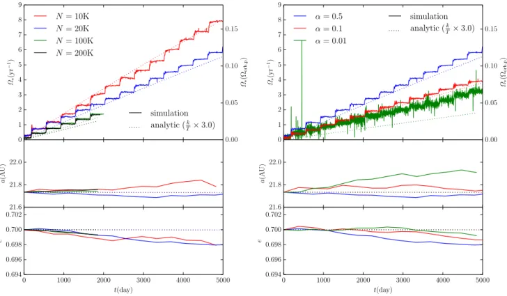
In Fig.5we present the evolution of∗,aandeover a period of 5000 d (∼13 orbits). All simulations use the initial conditions of model O0R37 while we variedN(left-hand figure) andα (right-hand figure). It can be seen that for different values of these SPH parameters we find different values of ˙∗.
The difference in ˙∗can be understood by taking the radius of the star into account. Because of the quantization approximations inherent to SPH, a different value of Ncan result in a slightly different hydrodynamical balance within the star. This difference,
or even a different value ofα, can result in variation of the radius of the SPH realization of the star after relaxation. Even a small change inR∗can account for the differences in ˙∗because ˙∗∝R6
∗(Hut
1981).
While we do not include the physical processes that regulate tidal damping in our simulations, the artificial viscosity in SPH can cause dissipation. To interpret the results of our simulation, it is good to know how the time-scale of this artificial dissipation compares with the time-scale of realistic physical dissipation. The dotted line in Fig.5is a numerical integration of the analytical solution for the change in orbital parameters through tidal dissipation. In this analyt-ical solution, we have used the radius of the relaxed SPH realization of the star for each simulation. The analytical solution is close to the result of our simulation when we assumek/T=3×(k/T)Rasio,
which is within the uncertainty in the tidal damping time-scale. This is fortuitous because we can now directly compare the tidal dissipation in our simulations with a real physical system.
However, in the bottom panels of Fig. 5we see that the or-bit circularizes (edecreases) faster than what is predicted by the analytical models. We also see larger changes inathan what is predicted by the analytical models, but there is no clear trend in these changes. We have carefully examined these simulations and we find that these changes inaanderesult from errors in the to-tal energy (Etot) and angular momentum (Jtot) in the simulations.
These errors are typically of order E/Etot ∼ J/Jtot ∼ 10−4
per 1200 d, which is reasonable for a gravitational tree code with smoothing like the one inFI. However, in Fig.5we see that these
small errors have a larger effect on the orbital parameters than the tidal dissipation. We will therefore carefully examine the contribu-tion of these errors when we investigate the orbital evolucontribu-tion in Section 4.3.
4.2 Mass-loss
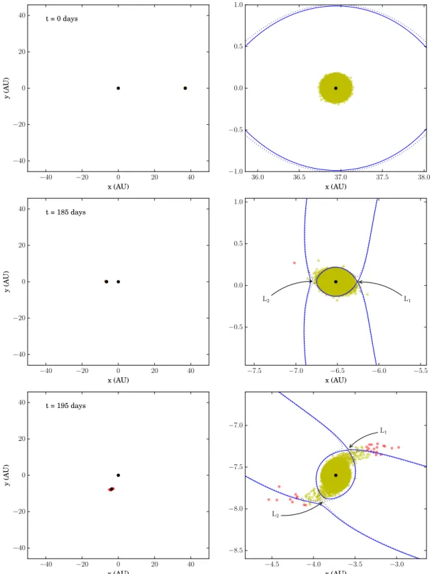
The star loses mass near pericentre in all simulations withR∗ RRoche. We present three snapshots of a simulation with relatively
high mass-loss rate (O1R43) in Fig.6as an example. At pericentre (t=185 d) the star fills its Roche lobe, but the mass is only lost after the pericentre passage.
Part of the stellar mass is lost through the second Lagrangian point (L2), instead of the first Lagrangian point (L1), which can be
seen in the bottom right-hand panel of Fig.6. The binary system we study has a high mass ratio and therefore the difference in gravitational potential between the L1and L2points is small. If the
stellar surface would follow an equipotential surface perfectly, this small difference in the gravitational potential would be enough to cause all mass to leave the star through the L1point. However, the
stellar surface layers have a finite thickness, so mass-loss through the L2 point is a physical possibility. In Fig. 7, we present the
fraction of mass lost through the L2point (fL2) in our simulations.
In simulations where the total mass-loss per orbit is large compared to the SPH particle mass, we find thatfL2≈0.4. For simulations
with lower mass-loss rate, there is a larger spread infL2, which is a
result of the limited resolution in those simulations.
Figure 5. The long-term evolution through tidal dissipation of∗,aandefor model O0R37 with varying values ofNandα. Dotted lines show the analytical solution for tidal dissipation (Hut1981) withk/T≈3(k/T)Rasio. Different values ofNandαresult in a different radius of the relaxed SPH realization of the star. The analytical solution matching each simulation is therefore calculated with the effective radius of the SPH realization of the star in that simulation. The simulations withN=100 000 and 200 000 are more computationally expensive and we have therefore decided to run them for only 2000 d. Note that the blue line in both plots is the same simulation.
radius of the relaxed SPH realization of the star differs between the simulations with different resolution. Because the resolution affects the mass-loss rate, we will not draw any conclusions based on the absolute mass-loss rate; instead we focus on the effect of a given mass-loss rate on the orbital evolution.
Using Fig.8we confirm that the mass is mostly lost after peri-centre. We find that there is a time delay of up to 10 days between the Roche lobe overflow and the peak of the mass-loss for systems wheree=0.7. For systems wheree=0.95, we do not find any delay larger than our time resolution limit of 1 d. When the gas is grav-itationally accelerated during the pericentre passage, it takes some time before it becomes unbound. We suspect that this time delay is related to the hydrostatic time-scale (τhydr) of the star (Kippenhahn,
Weigert & Weiss2012). Indeed for the star used in simulations with e=0.7,τhydr≈2 d while for simulations withe=0.95, the smaller
star hasτhydr≈0.2 days.
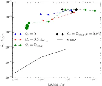
In Fig.9we present the mass-loss rate as a function of initial radius as calculated in Section 3.4. We find that the mass-loss rate is extremely sensitive to the radius (|M˙∗| ∝(R∗/RRoche)15.9). In fact,
most of the dependence of the mass-loss rate on the resolution seen in Fig.8can be accounted for by the difference in the effective radius. We find a spread of more than an order of magnitude around the ˙M∗–R∗ relationship, which could be partly due to numerical noise.
In Fig.10, we present the rate of change in the stellar radius ( ˙R∗) caused by the stellar mass-loss. Losing mass from the surface of the star results in a lower pressure at the stellar surface. This low pressure will cause the inner part of the SPH model to respond by expanding, and therefore the stellar radius increases during
mass-loss. This is also true, at least qualitatively, for a realistic star with a convective envelope, and therefore we have also plotted ˙R∗ cal-culated with the stellar evolution code (MESA) where we have set
an artificial mass-loss for the case in whichR∗=39 R. However, quantitatively ˙R∗is not the same because we do not have a realistic stellar structure. Our simulations do not include nuclear burning in the stellar core and in fact we have replaced the entire core with a single SPH particle. More importantly, we cannot fully resolve the steep density gradient at the edge of the star using SPH. The expansion of the star may also be affected by the gravitational in-teraction with the black hole. During this inin-teraction, orbital energy can be converted into heat, which can cause the star to expand. This process may be partly responsible for the stellar expansion in the SPH model, while it is not taken into account in theMESAmodel. We
show in Fig.10that the change in the radius of our SPH star is more than two orders of magnitude higher than what is calculated using
MESA. It is unclear which part of this difference is caused by the lack of a realistic stellar structure in our simulations, and which part is caused by the more realistic effect of the gravitational interaction. We therefore conclude that we cannot ensure that we can reliably simulate the system with mass-loss for a long period of time. Even during the 1200 d used in these simulations, we already see a slight increase in the mass-loss rate caused by the increase in the stellar radius.
Figure 6. The particle positions in the orbital plane for three snapshots of the simulation with model O1R43. In the left-hand panels, we present an overview while the right-hand panels zoom in on the star position. Black circles are the black hole and the stellar core, yellow and red circles are SPH particles bound and not bound to the star, respectively. The blue solid and dotted lines are approximate equipotential surfaces through L1and L2respectively. The top panel shows the apocentre position and the middle panel shows the pericentre position. The bottom panel shows that after the pericentre passage, particles leave the star through both the L1and L2points.
mass-loss. Despite the mass-loss, the general shape of the stellar density profile remains the same. This indicates that the time that the star is far from the black hole, is long enough for the stellar structure to adjust to the mass-loss.
4.3 Orbital evolution
Figure 7. The fraction of mass lost through the L2point (fL2) as opposed
to the L1point as a function of the total mass-loss rate. Sets of simulations where onlyR∗differs between them are connected by dashed lines. Larger symbols connected by dotted lines represent the higher resolution simula-tions listed in Table3. For smaller total mass-loss rate, there is a larger spread because only a small number of SPH particles are lost in this case. The general trend is that almost half the mass is lost through the L2point and moves away from the black hole.
Figure 8. Total mass and mass-loss rate of model O1R39 withN=20 000, 100 000 and 500 000 particles. The mass-loss rate is lower for simulations with a higher resolution.
Fig.12(top panel), we present the change in the angular momentum of the star ( J∗), the black hole ( JBH), and the matter that is not
bound to the star ( Junbound). The star and the black hole exchange
angular momentum periodically during the eccentric orbit while the star loses angular momentum due to the mass-loss. The error in the total angular momentum J/Jtot∼10−4just like in the simulations
without mass-loss, but the effect of mass-loss onJ∗is larger than the effect of this error.
In Fig.12(bottom panel), we distinguish between the angular momentum taken by matter leaving the star through L1( JL1) and
through L2( JL2). The matter leaves the star in opposite
direc-tions, but both remove a positive amount of angular momentum from the star, and therefore the effect on the star is cumulative. The combined angular momentum taken when matter leaves the star ( JL1+L2) is nearly equal to the angular momentum in the unbound
matter ( Junbound). We therefore conclude that the gravitational
in-Figure 9. The average mass-loss for different stellar radii (in units of the Roche radius). Only simulations with significant mass-loss are included. The dash–dotted line is a fit to these points, but note that the mass-loss is resolution dependent.
Figure 10. The expansion of the star in response to mass-loss in our sim-ulations compared to a stellar evolution model usingMESAwith artificial mass-loss. In our SPH simulations, ˙R∗is over two orders of magnitude higher than in theMESAmodel.
teraction after mass-loss between the star and the unbound matter is negligible.
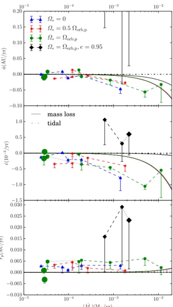
In Fig.13, we present the change in the orbital parametersa, eand pericentre distance (rp) of our simulations as a function of
Figure 11. The stellar density profile for model O1R45 at the apocentre passages of the simulation, compared to theMESAmodel. As mass is lost, the density at the edge of the star decreases, but the overall shape of the density profile remains the same.
Figure 12. The change in angular momentum in the orbital plane of the star, black hole and unbound gas for model O1R45 (top panel). The star and black hole exchange angular momentum because the orbit is eccentric and the star loses angular momentum that is taken by the mass that is lost. The total angular momentum is conserved, with an error of∼10−4Jtot. We also present details on different contributions to the angular momentum in the unbound gas (bottom panel). We compare the angular momentum taken by the mass as it is lost through L1and L2( JL1+ JL2= JL1+L2) with
the total angular momentum of the unbound gas ( Junbound).
Figure 13. The change in orbital parameters as a function of mass-loss rate for our simulations,e=0.7 unless otherwise specified. The error bars are based on the systematic errors inEtot andJtot, the details of these are discussed in the text. The solid and dash–dotted lines represent the analytical predictions for mass-loss (Sepinsky et al.2009) and tidal dissipation (Hut 1981), respectively. For the analytical prediction from mass-loss, we assume that the mass lost throughL2is not accreted on to the black hole. The tidal effects depend on the mass-loss rate because we have varied the radius with the mass-loss rate following the fit in Fig.9. In the top panel, the simulations withe=0.95 have ˙a∼0.9 au yr−1but due to the large errors the result are consistent with zero.
In the top two panels of Fig.13 we see thataandegenerally decrease for simulations withe=0.7, and that the rate of change is larger for larger mass-loss, which is qualitatively consistent with the analytical models. In the bottom panel, we see thatrpgenerally
increases with time at a higher rate than what is predicted by the analytical models but they appear to be consistent within the error bars. For the simulations withe=0.95, the errors are far larger because of the higher velocity and acceleration at pericentre that amplify the errors. We therefore cannot draw any conclusions about the orbital evolution of these systems.
With the higher value of ˙rpwe have measured, we can calculate
Figure 14. The observed X-ray light curve fromSwift(top, Godet et al. 2014), compared with the mass-loss through L1from two parts of simulation O1R43 (bottom). The start time is chosen to provide the closest match between the observations and the simulations.
of the change inR∗through stellar evolution with mass-loss from Fig.10, which is∼106yr. The change in the stellar orbit is clearly
much faster, and dominates the evolution of this system.
4.4 Comparison with observation
In Fig.14we compare the observed X-ray light curve with the mass-loss rate through L2as a function of time in simulation O1R43. We
cannot compare the mass-loss rate with the light curve directly because several processes, like the formation of an accretion disc, will modulate the signal. This accretion disc, and in particular the viscous time-scale of that disc, are an important and heavily debated part for most models of HLX-1 (see e.g. Soria2013). We cannot draw conclusions about the accretion disc from our simulations, however, we can compare our results with the observations if we make two assumptions. (1) The X-rays are caused by the mass that is lost from the star and the efficiency with which the mass is turned into X-rays does not differ noticeably between outbursts. (2) Any delay between the time of mass-loss and the time when X-rays are emitted does not differ between outbursts. It should be noted that accretion discs physics is very complex and therefore these assumptions do not necessarily hold for all accretion scenarios.
At the start of the simulation (tstart =0 d), the mass-loss rate
increases, which does not match the observations. After running the simulation for a longer time (tstart=5700 d), the mass-loss rate
starts to decrease, matching the observations, although the orbital period has changed by that time. Note however, that the long term mass-loss rate evolution is also influenced by numerical effects as discussed in Section 4.2.
The observed X-ray flux profile has a tail after every outburst while the simulated mass-loss rate only shows a sharp peak at each outburst. The observed tail is probably caused by an accretion disc
that can delay the accretion of material on to the black hole. Based on this assumption, Soria (2013) have calculated that the accretion disc has a radius of∼15 R. This is an order of magnitude lower than the radius estimate based on the observed continuum emission from the hot disc. This discrepancy is still an unsolved issue in most models for HLX-1 and our simulations are not able to resolve that. It is important to note that our simulations cannot explain the observed delay of over 30 and 60 days in the last two outburst. Despite the fast evolution of the orbit, and particularly rp, such
strong variations do not occur in our simulations.
5 D I S C U S S I O N A N D C O N C L U S I O N
The analytical solutions that have been used so far to investigate the orbital evolution of eccentric binaries during mass transfer are not sufficient to predict the orbital evolution of the HLX-1 system. Key assumptions in the analytical mass-loss model, that all mass is lost through the L1point at pericentre and that the mass transfer happens
instantaneously, turn out to be incorrect. The orbital evolution in our simulations is faster than what is predicted by analytical models but within the numerical errors they are still consistent. However, even with full hydrodynamical mass transfer simulations we are unable to explain the observed delay of over 30 d in the last outburst.
The density near the edge of the star, and therefore ˙M∗, depends on the number of SPH particles used in our simulation (Figs 4 and8). We are therefore not able to investigate the mass-loss rate as a function of stellar radius ( ˙M∗(R∗)). However, the goal of this research is to investigate the orbital evolution of HLX-1, not the mass-loss rate of the star. To account for the uncertainty in ˙M∗(R∗), we only investigate the change in orbital parameters as a function of ˙M∗, not as a function ofR∗. We also note that the time-scale of tidal damping is within the range of theoretical expectations, although this is probably coincidental as the detailed physics of tidal dissipation is not accounted for in our work (Section 4.1).
We have shown that the error in angular momentum (and en-ergy) is small ( J/Jtot ∼10−4, Fig.12), but that this still has a
considerable effect on the orbit. The change in the orbital angular momentum due to this error is larger than the change due to tidal dissipation, but smaller than the change due to mass-loss. There-fore, we have reason to believe that apart from these errors, our simulations provide a reliable prediction for the orbital evolution of HLX-1. We obtain the following results.
(i) Approximately 40 per cent of the stellar mass is lost through the L2point instead of through the L1point and this mass carries
approximately 40 per cent of the angular momentum that is lost from the star. This agrees with the results for mass transfer in eccentric binaries (Regos et al.2005; Lajoie & Sills2011). The analytical models for binary evolution could be improved by taking this into account. The angular momentum carried by the mass lost through the L1 point and the L2point have the same sign. Therefore, the
effect of the mass-loss through L1and L2 on the stellar orbit is
cumulative.
(iii) Whene=0.7, we find that the semimajor axis (a) and eccen-tricity (e) generally decrease, and this decrease is faster for higher mass-loss rates, which is qualitatively consistent with analytical models. In nearly all models, we find that the pericentre distance (rp) increases faster than what is predicted by analytical models, but
within the error they are still consistent.
(iv) Whene= 0.95, the behaviour of our simulations is very different from what is predicted by analytical models. However, the errors in energy and angular momentum become so large that we cannot draw any conclusions regarding the loss of angular momen-tum.
(v) We cannot explain the observed delay in the outbursts of HLX-1 as a change in the orbit seen in our simulations, despite the fast changes in the orbit that we do see.
If we take the increase inrpthat we have found in our simulations
at face value, we can use this to constrain the possible formation mechanisms of the HLX-1 system. An increase inrpcan cause a
decrease in the mass-loss rate if no other processes would affect the mass-loss rate. At the start of our simulations, we instead see an increase of the mass-loss rate but this is most likely caused by the unphysical expansion of the star. If the mass-loss rate would indeed decrease, then this would qualitatively agree with the obser-vation that the total outburst fluence decreases. However, the value of ˙rpwe find is very high and therefore the mass-loss rate would
decrease very quickly under this assumption. Extrapolating back in time, the mass-loss should have started within the last∼10 yr to avoid unphysically high mass-loss rates in the past if the value of ˙rpwe measured is correct. This conclusion agrees with the fact
that HLX-1 was not detected inROSATobservations in the early 90s (Webb et al.2010). The change in radius through stellar evo-lution is too slow to have initiated the mass transfer. However, we cannot exclude the possibility that a change in the stellar ro-tation, caused by tidal dissipation, could have initiated the mass transfer.
If the star did not evolve on the current orbit, it could have been captured by the black hole within the last∼10 yr. This could have happened through tidal capture as discussed below. Another pos-sibility is that a binary was disrupted by the black hole, leaving one star on an eccentric orbit, while the other star escaped the sys-tem. The probabilities for both these scenarios are largely unknown (but see Caputo D. P. et al., in preparation). Recently, alternative scenarios have also been proposed, such as wind accretion (Miller et al.2014) and extreme super-Eddington accretion on a stellar mass object (King & Lasota2014).
We can compare our results with the results from the work by Godet et al. (2014) as our investigation and methods are similar. We should take into account that we have used very different ini-tial conditions and therefore have investigated a different scenario. The most important difference in our results is that we do not see large stochastic variations in the orbital period, which could simply be due to the far lower eccentricity used in this work. However, it could also be a result of the artificial viscosity; we have used
α=0.5, while Godet et al. (2014) did not use artificial viscosity at all. This choice was made by them because artificial viscosity might lead to unphysical damping of stellar oscillations (Lombardi et al.1999). We note however, that viscous processes in real stars are only partially understood. This different choice for the artificial viscosity is important because it affects the tidal dissipation as we have discussed above. They do not discuss the possibly unphysical radius expansion we have noted in Section 4.2, although we suspect that it also affects the long term evolution of ˙M∗ in their
simula-tion. The effects of the energy and angular momentum errors are important to note, because we have found that these errors are far larger when the eccentricity is higher, and their model has an even higher eccentricity than what we have investigated. However, they calculate gravity with direct summation and find E/Etot10−4
and J/Jtot10−7which cannot explain the orbital evolution they
find (Lombardi, private communication).
Since the mass of the donor star is not constrained by observa-tions, we have also experimented withMZAMS=20 M. We have
tried this with bothe=0.7 and 0.95 and withR∗determined using Fig.1. However, these simulations were plagued by numerical in-stabilities. The difficulty we experienced in acquiring a dynamically stable solution may reflect a problem in the numerical methods. The high eccentricity in these orbits makes it very hard to integrate the equations of motion properly. In one of these cases we were able to acquire a numerically stable solution, but in that case the evolution ofaandebehaved very unexpectedly and we were unable to deter-mine if this was due to numerical issues or because such a system is intrinsically unstable. We have therefore omitted these results from this study.
We have also attempted to extend the evolution of the system beyond three orbits in order to study the long-term evolution of the mass transfer process. However, as we show in Fig.10, the stellar radius does not evolve realistically using the SPH method. This raises the question if the SPH method is at all suitable to follow more than a single pericentre passage properly. In our simulations
˙
R∗4×10⁻³Ryr−1, which corresponds to an 0.003 per cent
increase during the 1200 days over which we run our simulations. Since|M˙∗| ∝(R∗/RRoche)15.5, this radius increase is responsible for
a 0.5 per cent increase in the mass-loss rate. This is still a moderate error, but if we were to run for a much longer time, the increase in mass-loss would accelerate the stellar radius expansion, resulting in a runaway process and this error would begin to dominate. We have therefore decided not to run our simulation for longer than 1200 d in order to prevent the numerical method from directly influencing the measured mass-loss rate in the simulations. Realizing this numerical effect, we have not interpreted the change in the mass-loss rate in our comparisons with the observations.
To further improve our understanding of the orbital evolution of HLX-1, more simulations are required that address the caveats dis-cussed in this work. Many of the initial parameters are unknown and we have only investigated a small subset of the possible values. A much larger set of these simulations, while computationally expen-sive, could reveal trends in the orbital evolution, and provide further understanding of the mechanisms involved. However, the large un-certainties in both the initial parameters and the accretion scenario in general as well as the numerical errors, should be addressed first. One way to address the numerical errors in energy and angular momentum would be to replace the gravitational tree method with a directN-body method. In a tree method, the gravitational force from sets of distant particles is approximated as the force from a single mass. In a directN-body method, the gravitational force from each particle is calculated separately. While more computationally expensive, this would improve the accuracy of the method and solve some of the problems encountered in this work (for a comparison, see e.g. B´edorf, Gaburov & Portegies Zwart2012).
therefore seems unlikely that the periodicity in the outbursts corre-sponds to the period of an orbit as it is investigated here.
AC K N OW L E D G E M E N T S
We thank the anonymous referee for critical reading that helped us to improve the manuscript. This work was supported by the Netherlands Research Council NWO (grants no. 643.200.503, no. 639.073.803 and no. 614.061.608) and by the Netherlands Research School for Astronomy (NOVA).
R E F E R E N C E S
Barlow R., 2004, preprint (arXiv:e-prints)
Bate M. R., Bonnell I. A., Price N. M., 1995, MNRAS, 277, 362 Baumgardt H., Hopman C., Portegies Zwart S., Makino J., 2006, MNRAS,
372, 467
B´edorf J., Gaburov E., Portegies Zwart S., 2012, J. Comput. Phys., 231, 2825
Belczynski K., Kalogera V., Rasio F. A., Taam R. E., Zezas A., Bulik T., Maccarone T. J., Ivanova N., 2008, ApJS, 174, 223
Church R. P., Dischler J., Davies M. B., Tout C. A., Adams T., Beer M. E., 2009, MNRAS, 395, 1127
Davis S. W., Narayan R., Zhu Y., Barret D., Farrell S. A., Godet O., Servillat M., Webb N. A., 2011, ApJ, 734, 111
de Vries N., Portegies Zwart S., Figueira J., 2014, MNRAS, 438, 1909 Eggleton P. P., 1983, ApJ, 268, 368
Eggleton P. P., Kiseleva L. G., Hut P., 1998, ApJ, 499, 853
Farrell S. A., Webb N. A., Barret D., Godet O., Rodrigues J. M., 2009, Nature, 460, 73
Farrell S. A. et al., 2014, MNRAS, 437, 1208
Godet O., Barret D., Webb N. A., Farrell S. A., Gehrels N., 2009, ApJ, 705, L109
Godet O. et al., 2012, ApJ, 752, 34
Godet O., Lombardi J. C., Antonini F., Barret D., Webb N. A., Vingless J., Thomas M., 2014, ApJ, 793, 105
Hut P., 1981, A&A, 99, 126
Ivanov P. B., Papaloizou J. C. B., 2004, MNRAS, 347, 437 King A., Lasota J.-P., 2014, MNRAS, 444, L30
Kippenhahn R., Weigert A., Weiss A., 2012, Stellar Structure and Evolution. Springer-Verlag, Berlin
Kong A. K. H., Soria R., Farrell S. A., 2015, Astron. Telegram, 6916, 1 Lajoie C.-P., Sills A., 2011, ApJ, 726, 67
Lasota J.-P., Alexander T., Dubus G., Barret D., Farrell S. A., Gehrels N., Godet O., Webb N. A., 2011, ApJ, 735, 89
Lombardi J. C., Sills A., Rasio F. A., Shapiro S. L., 1999, J. Comput. Phys., 152, 687
MacLeod M., Ramirez-Ruiz E., Grady S., Guillochon J., 2013, ApJ, 777, 133
Meibom S., Mathieu R. D., 2005, ApJ, 620, 970
Miller M. C., Colbert E. J. M., 2004, Int. J. Mod. Phys. D, 13, 1 Miller M. C., Farrell S. A., Maccarone T. J., 2014, ApJ, 788, 116 Monaghan J. J., 1992, ARA&A, 30, 543
Morris J. P., Monaghan J. J., 1997, J. Comput. Phys., 136, 41
Paxton B., Bildsten L., Dotter A., Herwig F., Lesaffre P., Timmes F., 2011, ApJS, 192, 3
Pelupessy F. I., 2005, PhD thesis, Leiden Observatory
Pelupessy F. I., van Elteren A., de Vries N., McMillan S. L. W., Drost N., Portegies Zwart S. F., 2013, A&A, 557, 84
Peters P.-C., 1964, Phys. Rev. B, 136, 1224
Portegies Zwart S. F., Verbunt F., 2012, Astrophysics Source Code Library, record ascl:1201.003
Portegies Zwart S., McMillan S. L. W., van Elteren E., Pelupessy I., de Vries N., 2013, Comput. Phys. Commun., 183, 456
Price D. J., 2012, J. Comput. Phys., 231, 759
Rasio F. A., Tout C. A., Lubow S. H., Livio M., 1996, ApJ, 470, 1187 Regos E., Bailey V. C., Mardling R., 2005, MNRAS, 358, 544 Reimers D., 1975, Mem. Soc. R. Sci. Liege, 8, 369
Sepinsky J. F., Willems B., Kalogera V., 2007a, ApJ, 660, 1624
Sepinsky J. F., Willems B., Kalogera V., Rasio F. A., 2007b, ApJ, 667, 1170 Sepinsky J. F., Willems B., Kalogera V., Rasio F. A., 2009, ApJ, 702, 1387 Servillat M., Farrell S. A., Lin D., Godet O., Barret D., Webb N. A., 2011,
ApJ, 743, 6
Shakura N. I., Sunyaev R. A., 1973, A&A, 24, 337 Soria R., 2013, MNRAS, 428, 1944
Soria R., Hau G. K. T., Pakull M. W., 2013, ApJ, 768, L22
Straub O., Godet O., Webb N., Servillat M., Barret D., 2014, A&A, 569, 116
van Elteren A., Pelupessy I., Portegies Zwart S., 2014, Phil. Trans. R. Soc. A, 372, 30385
Webb N. A., Barret D., Godet O., Servillat M., Farrell S. A., Oates S. R., 2010, ApJ, 712, L107
Webb N. et al., 2012, Science, 337, 554
Wiersema K., Farrell S. A., Webb N. A., Servillat M., Maccarone T. J., Barret D., Godet O., 2010, ApJ, 721, L102
Zahn J.-P., 1977, A&A, 57, 383