Zhepu Zhao. A comparison study: Comparison Between Different Classifiers for Emotion Classification Using Real Human-to-Human Chat Log Dataset. A Master’s Paper for the M.S. in I.S degree. April, 2019. 41 pages. Advisor: Jaime Arguello
In the field of emotion classification in natural language processing, researches usually concentrate on the datasets which are more academic and formal like Stack Overflow and general reviews on products or ideas like Tweeter and Amazon, but lack analysis in datasets which come from real, private, human-to-human chat logs or oral conversation. For this study, we implemented four types of commonly used classifier with a dataset which consists of both text from chat logs and oral conversations that are transformed into script. Meanwhile, we analyzed the performance of different classifiers across these two types of datasets. Specifically, we used BOW (Bag of words) and its extended version considering TF-IDF for future analysis. We found that the performance of the logistic regression does not depend too much on the dictionary size of BOW and all four types of classifiers perform better in text from user’s typing than in text transformed from oral conversations.
Headings: NLP
Emotion Classification Bag of Words
A COMPARISON STUDY: COMPARISON BETWEEN DIFFERRENT CLASSIFIERS FOR EMOTION CLASSIFICATION USING REAL HUMAN-TO-HUMAN CHAT
LOG DATASET
by Zhepu Zhao
A Master’s paper submitted to the faculty of the School of Information and Library Science of the University of North Carolina at Chapel Hill
in partial fulfillment of the requirements for the degree of Master of Science in
Information Science.
Chapel Hill, North Carolina April 2019
Approved by
Introduction
With the advent of the enormous growth of digital content in the Internet, text in the digital format has received more and more attention in information retrieval and natural language processing community. This kind of work has focused on topical categorization, attempting to sort documents according to their subjects (such as economics and politics) (Pang et al., 2002). However, many researchers have been turned their attention to some other hidden information within the text. Emotion is exactly part of the hidden information behind the text.
People’s emotion could vary greatly in certain circumstances. For one person, his/her
emotion could be different in different situations. Even under the same situation, different people could have different emotions. People communicate with each other a lot every day and their emotions could be influenced by the conversation they are in. Because there are some many changes and uncertainty within emotions, with the goal of learning more about emotion within the text, emotion processing in text gradually becomes a hot and active area in the field of Natural Language Processing (NLP). More specifically, Textual emotion detection or classification becomes a task on which many scholars and researcher concentrate.
Researches in the field of textual emotion classification have fallen into two major categories. One (“machine learning techniques”) (Mullen & Collier, 2004) attempts to train
the words in the documents. The other method (“semantic orientation”) (Whitelaw, Garg,
& Argamon, 2005), which is also named as keyword-based classification (Kao et al., 2009) is used to detect emotions based on the related set(s) of keywords found in the input text (Kao et al., 2009). Usually, it is applied to classify words into two classes, such as “positive” or “negative”, and then count an overall positive/negative score for the text. If
the number of positive terms in a specific document is more than the number of negative terms, it is labeled as positive. Likewise, if the number of negative terms in the document is more than the number of positive terms, it is assigned as negative.
Many researches concentrate on the classifiers or the models a lot. However, dataset is also a quite important factor that influences the training results. To detect people’s emotion,
there are different ways to apply. Concretely, in general, there are three methods to detect emotions (Soleymani et al., 2017). The first is the speech. Different audio processing tools could analyze multiple factors like pitch and loudness within an audio file. The second one is the visual tools like video and pictures. We might identify emotions from people’s face
expression and body movements. The last one is the text. People communicate with each other both digitally and orally every day and both of these two ways could be transferred and stored in digital text for analyze.
For this study, we’re planning to focus on textual emotion classification. There are some
different classifiers and evaluate the performance of them with a specific MultiClass strategy, One-Vs-The-Rest. Specifically, according to our dataset, we have 8 categories of emotions in total: neutral, non-neutral, disgust, surprise, joy, sadness, fear, and anger. Besides, we compare the performance of a given classifier under two types of text dataset: (1) dataset coming directly from people’s typing. For example, data from texting
application. (2) dataset coming from script converted from audio.
Related Work
Emotion classes
There are two major types of classification, binary classification (coarse-grained classification of sentiment polarity) and multi-class classification (fine-grained classification multiple classes) (Turner, 2000 and Plutchik, 1980).
of the French version of the State-Trait Anxiety Inventory (form Y) adapted for older adults. Vera-Villarroel did preliminary analysis based on normative data of the State-Trait Anxiety Inventory (STAI) in adolescent and adults of Santiago, Chile.
Emotion classification
There exist many types of emotion classifications.
Ackermann et al., 2016 mentioned an EEG-based (electroencephalography) automatic emotion detection method to classify emotions. Concretely, they evaluated the use of state-of-the-art feature extraction, feature selection and classification algorithms for EEG emotion classification using data from the de facto standard dataset, DEAP.
For our major concern, there are many researches concerning classifying emotions in different kinds of text, such as news reports, product reviews, and customer feedbacks. Generally, there are two common approaches: rule-based one and a machine-based one (Li & Xu, 2014).
A rule-based system that labels emotions in news headlines was proposed and implemented by (Chaumartin, 2007). It computes word’s sentiment polarity according to linguistic knowledge and predefined rules. The system has a high accuracy, but the recall of the system is rather low.
For the learning-based approach, (Tan & Zhang, 2008) explored four feature selection methods (MI, IG, CHI and DF) and
Rao et al. (2016) proposed a topic-level maximum entropy (TME) model for social emotion classification over short documents. TME generates topic-level features by modeling latent topics, multiple emotion labels, and valence scored by numerous readers jointly. The overfitting problem in the maximum entropy principle is also alleviated by mapping the features to the concept space.
Li & Xu (2014) described an SVR and SVM-based emotion classifier with feature selection using emotion causes. They basically combined rule-based and learning-based methods together. After thorough analysis on sample data they constructed an automatic rule-based system to detect and extract the cause event of each emotional post. Then, they used corpus built up by themselves to train the classifier.
Methodology
This section presents the methodology of emotion classification. Before defining and implementing different classifiers, we need to prepare the data first and determine the input features of the data. These two sub-sections will be explained in details in the next section. For this section, we mainly focus on learning emotion classifiers via some common and frequently used learning-based approaches.
For this study, we focus on the multi-class classification task. Each utterance (one sentence or paragraph from a person) is labeled with one and only one sentiment category among eight categories from the dataset we chose. Basically, there are two strategies to implement multi-class classification which are One-VS-Rest and One-VS-One. The basic idea of One-VS-Rest strategy is that we choose one class and then lump all the others into a single second class. We do this repeatedly, applying different binary classification schemas to each case. The major reason we use these strategies is because of its interpretability. Since each class is represented by one and only one classifier, it is possible to gain knowledge about the class by inspecting its corresponding classifier.
Experiment results
Dataset
Currently, a labeled dataset called “EmotionLines” is available. The dataset is in the format of json and each utterance is labeled with one type of emotion categorized by (Chen et al., 2018). The dataset consists of two parts. One is from the scripts of a famous TV shows – Friends from season 1 to 9. The other is the real, private, human-to-human chat logs which are from conversations between friends on Facebook Messenger collected by an application called EmotionPush. All conversations are carried out in text form. The basic information of these two datasets are described in Table 1.
Friends EmotionPush
train validation test train validation test Number of Dialogue 720 80 200 720 80 200 Number of Utterance 10561 1178 2764 10733 1202 2807
Table 1 Dataset Information
# of Utterances
Emotion Label Distribution (%)
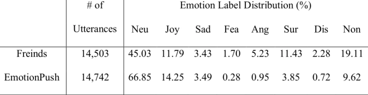
Neu Joy Sad Fea Ang Sur Dis Non Freinds 14,503 45.03 11.79 3.43 1.70 5.23 11.43 2.28 19.11 EmotionPush 14,742 66.85 14.25 3.49 0.28 0.95 3.85 0.72 9.62
Table 2: Detailed Information of the two sub datasets
The eight sentiment categories are: Neu (Neutral), Joy, Sadness (Sad), Fea (Fear), Ang (Anger), Sur (Surprise), Dis (Disgust), Non (Non-neutral).
The dataset is split into three sets: train, validation, and test. One of the most known difficulties when working with natural language data is that it is unstructured. For example, if we use it "as is" and extract tokens just by splitting the titles by whitespaces, we will see that there are many "weird" tokens. To get rid of the problem, it's usually useful to prepare the data somehow before training the classifier.
Performance Measure
To evaluate the performance of an emotion classifier, we use several metrics including F1 Score (macro, micro, and weighted) and accuracy score. Concretely, these metrics are computed with the following equations.
𝐹1 = 2 ∗ 𝑅𝑒𝑐𝑎𝑙𝑙 ∗ 𝑃𝑟𝑒𝑐𝑖𝑠𝑖𝑜𝑛𝑅𝑒𝑐𝑎𝑙𝑙 + 𝑃𝑟𝑒𝑐𝑖𝑠𝑖𝑜𝑛
𝐴𝑐𝑐𝑢𝑟𝑎𝑐𝑦 = 𝑛𝑢𝑚𝑏𝑒𝑟 𝑜𝑓 𝑎𝑐𝑐𝑢𝑟𝑎𝑡𝑒 𝑝𝑟𝑒𝑑𝑖𝑐𝑡𝑖𝑜𝑛𝑡𝑜𝑡𝑎𝑙 𝑛𝑢𝑚𝑏𝑒𝑟 𝑜𝑓 𝑝𝑟𝑒𝑑𝑖𝑐𝑡𝑖𝑜𝑛𝑠
For macro-F1, we calculate metrics for each "class" independently, and find their unweighted mean.
For weighted-F1, we calculate metrics for each label, and find their average weighted by support (the number of true instances for each label). This alters ‘macro’ to account for
label imbalance;
The micro-F1 and macro-F1 emphasizes the performances of the classifier on common and rare categories, respectively. Based on these two metrics, we can observe how the classifier works for different kinds of data.
Experiment Design
Data preparation
Firstly, we prepare the data by using some regular expression libraries to remove bad symbols like “/(){}\[\]\|@,;”. Then, we need to remove stop words which have very high
frequency and usually don’t have real meanings. Concretely, we use python libraries
including “nltk” and “re” to finish this data preprocessing task.
Next step is to transform the text data into vectors. Machine learning algorithms work with numeric data and we cannot simply use the raw text data to train the classifier. There are many ways to transform text data into numeric vectors. For our implementation, we will use two approaches.
Bag of words
1. Find N most popular words in train corpus and numerate them. Now we have a dictionary of the most popular words.
2. For each utterance in the corpora create a zero vector with the dimension equals to N.
3. For each text in the corpora iterate over words which are in the dictionary and increase by 1 the corresponding coordinate.
TF-IDF extends Bag of words
The second approach extends the bag-of-words framework by taking the frequencies of words in the corpora into account. This approach helps to penalize too frequent words and provide better feature space.
TF-IDF is the abbreviation of term frequency – inverse document frequency.
TF (Term frequency) represents the frequency for a term (or n-gram) t in document d. The notion is 𝑡𝑓(𝑡, 𝑑). There are different weighting schemes to represent TF weight shown in the Table 3. For our implementation, we pick the third one in the table.
Weighting Scheme TF Weight
Binary 0, 1
Raw count 𝑓𝑡,𝑑
Term frequency 𝑓𝑡,𝑑
∑𝑡′∈𝑑𝑓𝑡′,𝑑
Log normalization 1 + log (𝑓𝑡,𝑑)
IDF (Inverse Document Frequency) is incorporated which diminishes the weight of terms that occur very frequently in the document set and increases the weight of terms that occur rarely. IDF is calculated in the following way:
𝑖𝑑𝑓(𝑡, 𝐷) = 𝑙𝑜𝑔|{𝑑 ∈ 𝐷: 𝑡 ∈ 𝑑}|𝑁
𝑁 = |𝐷| (𝑡𝑜𝑡𝑎𝑙 𝑛𝑢𝑚𝑏𝑒𝑟 𝑜𝑓 𝑑𝑜𝑐𝑢𝑚𝑒𝑛𝑡𝑠 𝑖𝑛 𝑐𝑜𝑟𝑝𝑢𝑠)
|{𝑑 ∈ 𝐷: 𝑡 ∈ 𝑑}|= 𝑛𝑢𝑚𝑏𝑒𝑟 𝑜𝑓 𝑑𝑜𝑐𝑢𝑚𝑒𝑛𝑡𝑠 𝑤ℎ𝑒𝑟𝑒 𝑡ℎ𝑒 𝑡𝑒𝑟𝑚 𝑡 𝑎𝑝𝑝𝑒𝑎𝑟𝑠
We calculate TF-IDF as follows: 𝑡𝑓𝑖𝑑𝑓(𝑡, 𝑑, 𝐷) = 𝑡𝑓(𝑡, 𝑑) ∗ 𝑖𝑑𝑓(𝑡, 𝐷)
A high weight in TF-IDF is reached by a high term frequency (in the given document) and a low document frequency of the term in the whole collection of documents. We replace the value in the bag of words with TF-IDF calculated in the equation mentioned above.
Applying classifier
After preparing the data and transforming the features into numeric vectors, we need to use the prepared data to train the classifier. For this study, we plan to train the classifiers based on the strategy we mentioned in the previous chapter: One-VS-Rest Strategy.
One-VS-Rest Strategy involves training a single classifier per class, with the samples of that class as positive samples and all other samples as negatives. This strategy requires the base classifiers to produce a real-valued confidence score for its decision, rather than just a class label.
Inputs:
• 𝐿, a training algorithm for binary classifier
• Pre-prepared training data 𝑋
• Label set (classes) 𝑦 where 𝑦𝑖 ∈ {1, … , 𝐾} is the class label for the sample 𝑋𝑖
Outputs:
• A list of classifiers 𝑓𝑘 for 𝑘 ∈ {1, … , 𝐾}
Procedure:
• For each 𝑘 in {1, … , 𝐾}
o Construct a new label vector 𝑧 where where 𝑧𝑖 = 𝑦𝑖 if 𝑦𝑖 = k and 𝑧𝑖 = 0. o Otherwise, apply 𝐿 to 𝑋, 𝑧 to obtain 𝑓𝑘
Making decisions means applying all classifiers to an unseen sample x and predicting the label k for which the corresponding classifier reports the highest confidence score:
𝑦̂ = argmax 𝑘 in {1,…,𝐾}𝑓𝑘(𝑥)
To implement this strategy, we apply different strategies implemented by Scikit-learn, a free software machine learning library for the Python programming language. Specifically, we apply the class (OneVsRestClassifier) under package sklearn-multiclass to implement the multiclass classifier. The benefit of using this library is that it helps to balance the scale of the confidence value so that two confidence values are directly comparable. But there is also another problem of doing this. This will be discussed in the limitation section in the end.
Machine) Linear Classification model: Linear SVC (Support Vector Classification) Classifier. All four of these classifiers are referenced and implemented from sklearn.
Comparison and Analysis
For this section, we will analyze the experiment results. The analysis consists of three sections: (1) Compare the performance of different models within “EmotionPush”. (2)
Compare the performance of different models within “Friends”. (3) Considering BOW
(Bag of Words) and TF-IDF separately, compare different models across the two datasets. For the first two sections, we split the analysis process into three sub-steps: (1) Under One-vs-Rest strategy, we compared the performance of 4 models applied by different input features: TF-IDF and BOW. Also, we explore the difference among 4 models for the given input features: TF-IDF or BOW. (2) Under One-vs-One strategy, we do the same thing as One-vs-Rest by only replacing the models applied for One-vs-One strategy. (3) Given a input features (TF-IDF or basic BOW), we compare the performance between the two strategies (One-vs-Rest and One-vs-One).
Dataset EmotionPush Analysis
Under the One-vs-Rest strategy, we applied four models in total which are LinearSVC, logistic regression, Ridge regression, and SGD. We saved the running results in the format of csv and drew the line charts in Excel. Figure 1 - 3 show the three kind of F1 metric scores with basic BOW as input features.
represents the number of popular terms in the corpora. For example, we choose dictionary size as 500, then we pick top 500 terms in the corpora instead of using all of them. This is alternative method to test how much the classifier depends on the dataset size. An assumption we made for this is that the bigger the dataset is, the more popular words it will have.
Figure 1
Figure 3
For each metric score, SGD classifier and LinearSVC perform better than the other two models on average in F1-Micro. We can directly see that logistic regression model performs better than the other three and LinearSVC does the worst among four models. The score of F1-Macro of the other three models except logistic regression has the tendency to decrease as the size of dictionary size goes up, especially the LinearSVC and Ridge classifier. Thus, these two models have their optimal dictionary size which is around 500. This means to pick the top 500 popular words to construct the BOW will help the LinearSVC and ridge classifier get the highest F1-Macro score. For F1-weighted score, the broken lines represented different models intertwine with each other as the size of dictionary goes up to around 500.
Across these three figures, we found out that the score of all three kinds of metric is relatively low with small size of dictionary. However, as the size increases, the score will not increase infinitely. It fluctuates within a certain range or even drop down.
Figure 4
By comparing the metric score across different models, we can see that different models don’t behave too differently considering f1-micro and f1-weighted value. But logistic
regression performs a bit worse than the other three models in f1-macro value.
Figure 6
Figure 7
Figure 5 to Figure 7 showed the comparison between TF-IDF and basic BOW across different models in different F1 score. For LinearSVC, ridge classifier, and SGD, TF-IDF performs better for all three kinds of F1 score. However, BOW benefits more from logistic regression in F1-weighted and F1-macro and performs worse in F1-micro.
For this section, we replace the dataset “EmotionPush” with “Friends” and applied four
models used in the prior section. We also saved the running results in the format of csv and drew the line charts in Excel. Figure 8 - 10 show the three kind of F1 metric scores with basic BOW as input features.
From figures below, we can see that Logistic Regression is the most stable classifier in spite of the dictionary size which means it is less likely to fluctuate as the size of dictionary goes up. On the contrary, SGD classifier is more likely to fluctuate.
Figure 8
Figure 10
Considering different metric scores, logistic regression gets the highest value in F1-Micro compared to the other 3 models but performs worst in F1-Macro among four models. Not like the score of F1-Macro from dataset “EmotionPush”, F1-Macro value in this case doesn’t have the tendency to decrease as the size of dictionary size goes up. Thus, no
models have their optimal dictionary size in this case. This means we are able to improve the performance of the classifier in F1-Macro value by picking up certain value of dictionary size. For F1-weighted score, the broken lines represented different models intertwine with each other as the size of dictionary goes up to around 2500.
Across these three figures, we found out that the score of F1-Macro and F1-weighted is relatively low with small size of dictionary. However, as the size increases, the score will not increase infinitely. It fluctuates within a certain range or even drop down. But not like Micro in “EmotionPush” results, the dictionary size does not influence the value of F1-Micro too much.
Figure 11
By comparing the metric score across different models, we can see that the shape of the broken lines representing f1-macro and f1-weighted are quite similar. Concretely, logistic regression has the lowest value of these two metrics. But it has the best f1-micro value among four models.
Figure 13
Figure 14
Analysis across datasets
This section, we will compare the performance of different models across two datasets. The basic rule to make comparison is that for each type of f1 score, for example f1-macro, we keep the input features same, i.e. we only consider BOW or TF-IDF, then we draw the line charts according to the f1-macro score of different models across “EmotionPush” and “Friends”. As a result, we get figures shown from Figure 15.
Figure 15
models are more suitable for datasets which are more similar to “EmotionPush” rather than
“Friends”. There are two factors that can lead to this situation. Firstly, it could be that the
voice dataset is more heavily skewed towards a few categories, which would make it a more difficult dataset to work with. The other possible reason is that since all the utterances in “Friends” are transformed from audio script, while utterances in
“EmotionPush” are from users’ typing, it is possible that these classifiers perform better
for typed text rather than text transformed from script coming from audio or oral talking. Table 4 and Table 5 show the percentage of eight emotion categories under train, validation datasets.
EmotionPush neutral joy sadness fear anger surprise disgust
non-neutral
train 7148 1482 389 36 94 435 85 1064
validation 825 160 38 4 9 40 6 121
test 1882 458 87 2 37 93 15 233
Table 4 Percentage of emotion categories in EmotionPush
Friends neutral joy sadness fear anger surprise disgust neutral
non-train 4752 1283 351 185 513 1221 240 2017
validation 491 123 62 29 85 151 23 214
test 1287 304 85 32 161 286 68 541
Table 5 Percentage of emotion categories in Friends
Figure 16 Emotion Category Distribution Percentage in Train Set
Figure 17 Emotion Category Distribution Percentage in Validation Set
Figure 18 Emotion Category Distribution Percentage in Test Set
skewed Thus, our second assumption (classifiers we used probably perform better for typed text rather than text transformed from script coming from audio or oral talking) can be a better explanation for the difference between F1 score in “Friends” and “EmotionPush”
Conclusions and Limitations
In this work, we applied and tested the performance of four types of classifiers in total under One-vs-Rest Strategy with two types of datasets: “EmotionPush” and “Friends”. With the experiment results, we found some meaningful results as follows:
Firstly, considering different input features: the basic BOW and the extended BOW with TF-IDF as data entry, TF-IDF performs better than BOW in all three types of F1 score with LinearSVC, Ridge Classifier, and SGD Classifier. On the contrary, BOW performs better than TF-IDF in F1-Macro and F-Weighted with Logistic Regression.
Secondly, for the given input feature, BOW or TF-IDF, all three types of F1 score are higher in “EmotionPush” than in “Friends”. Since “EmotionPush” represents that dataset
coming directly from user’s typing and “Friends” represents dataset coming from script
transformed from audio, it is possible that all four types of classifiers perform better in text from user’s typing than in text in oral format.
Thirdly, the performance of different models varies for the given dataset and input feature. Thus, there isn’t absolutely best classifier that is suitable for all types of input
features and datasets. If the given input feature is BOW, logistic regression is the most stable model which means the dictionary size influences the F1 score least.
The limitation of this study is that we didn’t test other classification models in the field
Bibliography
Ackermann, P., Kohlschein, C., Bitsch, J. Á., Wehrle, K., & Jeschke, S. (2016, September). EEG-based automatic emotion recognition: Feature extraction, selection and classification methods. In 2016 IEEE 18th international conference on e-health networking, applications and services (Healthcom) (pp. 1-6). IEEE. Binali, H., Wu, C., & Potdar, V. (2010, April). Computational approaches for emotion
detection in text. In 4th IEEE International Conference on Digital Ecosystems and Technologies (pp. 172-177). IEEE.
Bishop, C. M. (2006). Pattern recognition and machine learning. springer.
Cambria, E. (2016). Affective computing and sentiment analysis. IEEE Intelligent Systems, 31(2), 102-107.
Cambria, E., & White, B. (2014). Jumping NLP curves: A review of natural language processing research. IEEE Computational intelligence magazine, 9(2), 48-57. Chaumartin, F. R. (2007, June). UPAR7: A knowledge-based system for headline
sentiment tagging. In Proceedings of the 4th International Workshop on Semantic Evaluations (pp. 422-425). Association for Computational Linguistics.
Chen, S. Y., Hsu, C. C., Kuo, C. C., & Ku, L. W. (2018). Emotionlines: An emotion corpus of multi-party conversations. arXiv preprint arXiv:1802.08379.
Chopade, C. R. (2015). Text based emotion recognition: A survey. International journal of science and research, 4(6), 409-414.
Chowdhury, G. G. (2003). Natural language processing. Annual review of information science and technology, 37(1), 51-89.
Devillers, L., & Vidrascu, L. (2006). Real-life emotions detection with lexical and paralinguistic cues on human-human call center dialogs. In Ninth International Conference on Spoken Language Processing.
Devillers, L., Lamel, L., & Vasilescu, I. (2003, July). Emotion detection in task-oriented spoken dialogues. In 2003 International Conference on Multimedia and Expo. ICME'03. Proceedings (Cat. No. 03TH8698) (Vol. 3, pp. III-549). IEEE. Ekman, P., & Friesen, W. V. (1971). Constants across cultures in the face and
emotion. Journal of personality and social psychology, 17(2), 124.
Hirat, R., & Mittal, N. (2015). A survey on emotion detection techniques using text in blogposts. International Bulletin of Mathematical Research, 2(1), 180-187.
Kao, E. C. C., Liu, C. C., Yang, T. H., Hsieh, C. T., & Soo, V. W. (2009, April). Towards text-based emotion detection a survey and possible improvements. In 2009
International Conference on Information Management and Engineering (pp. 70- 74). IEEE.
Kim, G. C. (1997). A dialogue analysis model with statistical speech act processing for dialogue machine translation. Spoken Language Translation.
extraction. Expert Systems with Applications, 41(4), 1742-1749.
Medhat, W., Hassan, A., & Korashy, H. (2014). Sentiment analysis algorithms and applications: A survey. Ain Shams engineering journal, 5(4), 1093-1113.
Mullen, T., & Collier, N. (2004). Sentiment analysis using support vector machines with diverse information sources. In Proceedings of the 2004 conference on empirical methods in natural language processing.
Pak, A., & Paroubek, P. (2010, May). Twitter as a corpus for sentiment analysis and opinion mining. In LREc (Vol. 10, No. 2010, pp. 1320-1326).
Pang, B., Lee, L., & Vaithyanathan, S. (2002, July). Thumbs up?: sentiment classification using machine learning techniques. In Proceedings of the ACL-02 conference on Empirical methods in natural language processing-Volume 10(pp. 79-86). Association for Computational Linguistics.
Plutchik, R. (1980). A general psychoevolutionary theory of emotion. In Theories of emotion (pp. 3-33). Academic press.
Rao, Y., Xie, H., Li, J., Jin, F., Wang, F. L., & Li, Q. (2016). Social emotion
classification of short text via topic-level maximum entropy model. Information & Management, 53(8), 978-986.
Soleymani, M., Garcia, D., Jou, B., Schuller, B., Chang, S. F., & Pantic, M. (2017). A survey of multimodal sentiment analysis. Image and Vision Computing, 65, 3-14. Tan, S., & Zhang, J. (2008). An empirical study of sentiment analysis for Chinese
documents. Expert Systems with applications, 34(4), 2622-2629.
Tripathi, S., Acharya, S., Sharma, R. D., Mittal, S., & Bhattacharya, S. (2017, February). Using Deep and Convolutional Neural Networks for Accurate Emotion
Classification on DEAP Dataset. In Twenty-Ninth IAAI Conference.
Turner, B. M. (2000). Histone acetylation and an epigenetic code. Bioessays, 22(9), 836 845.
Appendix – Classifier Implementation Codes
dataLoadAndProcess.py
import json import re
def data_load(train_path, val_path, test_path): """
:param train_path: :param val_path: :param test_path: :return train, val, test: """
# load raw data from json file with open(train_path) as train_data: train = json.load(train_data) # json.loads is only for string
with open(val_path) as validation_data: val = json.load(validation_data) with open(test_path) as test_data: test = json.load(test_data) return train, val, test
train, val, test = data_load('EmotionLines/EmotionPush/emotionpush_train.json', 'EmotionLines/EmotionPush/emotionpush_dev.json',
'EmotionLines/EmotionPush/emotionpush_test.json')
# extract emotion and utterance x_train = []
y_test = []
def text_extraction(train, val, test):
# extract utterance and emotions from the raw text data for ith_group in train:
for j in ith_group:
x_train.append(j['utterance']) y_train.append(j['emotion']) for ith_group in val:
for j in ith_group:
x_val.append(j['utterance']) y_val.append(j['emotion']) for ith_group in test:
for j in ith_group:
x_test.append(j['utterance']) y_test.append(j['emotion'])
return x_train, y_train, x_val, y_val, x_train, y_test
x_train, y_train, x_val, y_val, x_train, y_test = text_extraction(train, val, test)
def load_stopwords(): """
:return: stopwords """
file = open('english', 'r') stopwords = []
for line in file:
stopwords.append(line.split()[0]) return stopwords
# global variables
REPLACE_BY_SPACE_RE = re.compile('[/(){}\[\]\|@,;]') BAD_SYMBOLS_RE = re.compile('[^0-9a-z #+_]')
STOPWORDS = set(load_stopwords())
text = text.lower() # lowercase text
text = REPLACE_BY_SPACE_RE.sub(' ', text) # replace REPLACE_BY_SPACE_RE symbols by space in text
text = BAD_SYMBOLS_RE.sub('', text) # delete symbols which are in BAD_SYMBOLS_RE from text
text = ' '.join([word for word in text.split() if word not in STOPWORDS]) # delete stopwords from text
text = text.strip() return text
# prepare data
x_train = [text_prepare(x) for x in x_train] x_val = [text_prepare(x) for x in x_val] x_test = [text_prepare(x) for x in x_test]
# Dictionary of all emotions from train corpus with their counts. emotions_counts = dict()
for emotion in y_train:
# y_train represents list of 'emotion' list if emotion in emotions_counts:
emotions_counts[emotion] += 1 else:
emotions_counts[emotion] = 1
# Dictionary of all words from train corpus with their counts. words_counts = dict()
for item in x_train:
# X_train represents the 'utterance' string item_list = item.split(' ')
for word in item_list: if word in words_counts: words_counts[word] += 1 else:
words_counts[word] = 1 bagOfWords.py
from dataLoadAndProces import words_counts from dataLoadAndProces import emotions_counts from dataLoadAndProces import x_train
from dataLoadAndProces import y_test
from sklearn.preprocessing import LabelEncoder import numpy as np
from scipy import sparse as sp_sparse
from sklearn.feature_extraction.text import TfidfVectorizer DICT_SIZE = 700
# this is a dictionary
WORDS_TO_INDEX = dict()
# # words_frequency = sorted(words_counts.items(), key=lambda x: x[1], reverse=True)[:DICT_SIZE]
# words_frequency = sorted(words_counts.items(), key=lambda x: x[1], reverse=True) # index = 0
# for item in words_frequency:
# WORDS_TO_INDEX[item[0]] = index # index += 1
def my_bag_of_words(text, words_to_index, dict_size): """
text: a string
dict_size: size of the dictionary
return a vector which is a bag-of-words representation of 'text' """
result_vector = np.zeros(dict_size)
text = text.split() # split text string to a array of words for word in text:
if word in words_to_index:
result_vector[words_to_index[word]] += 1; return result_vector
# x_train_mybag = sp_sparse.vstack([sp_sparse.csr_matrix(my_bag_of_words(text, WORDS_TO_INDEX, DICT_SIZE))
# for text in x_train])
# x_val_mybag = sp_sparse.vstack([sp_sparse.csr_matrix(my_bag_of_words(text, WORDS_TO_INDEX, DICT_SIZE))
# for text in x_val])
# x_test_mybag = sp_sparse.vstack([sp_sparse.csr_matrix(my_bag_of_words(text, WORDS_TO_INDEX, DICT_SIZE))
# for text in x_test])
"""
"""
le = LabelEncoder()
y_train = le.fit_transform(y_train) y_val = le.fit_transform(y_val)
def tf_idf_features(X_train, X_val, X_test): """
X_train, X_val, X_test — samples
return TF-IDF vectorized representation of each sample and vocabulary """
# Create TF-IDF vectorizer with a proper parameters choice # Fit the vectorizer on the train set
# Transform the train, test, and val sets and return the result
tfidf_vectorizer = TfidfVectorizer(ngram_range=(1, 2), max_df=0.9, min_df=5, token_pattern='(\S+)')
X_train_tfidf = tfidf_vectorizer.fit_transform(X_train) X_val_tfidf = tfidf_vectorizer.transform(X_val) X_test_tfidf = tfidf_vectorizer.transform(X_test)
return X_train_tfidf, X_val_tfidf, X_test_tfidf, tfidf_vectorizer.vocabulary_
x_train_tfidf, x_val_tfidf, x_test_tfidf, tfidf_vocab = tf_idf_features(x_train, x_val, x_test)
tfidf_reversed_vocab = {i: word for word, i in tfidf_vocab.items()} application.py
from bagOfWords import x_train_tfidf from bagOfWords import x_val_tfidf from bagOfWords import x_train from bagOfWords import x_val from bagOfWords import x_test from bagOfWords import y_train from bagOfWords import y_val
from bagOfWords import my_bag_of_words from bagOfWords import WORDS_TO_INDEX from bagOfWords import words_counts
from sklearn import multiclass
from sklearn.gaussian_process import GaussianProcessClassifier from sklearn.gaussian_process.kernels import RBF
from sklearn import svm from sklearn import metrics
from scipy import sparse as sp_sparse import csv
def construct_bag_of_words(DICT_SIZE):
words_frequency = sorted(words_counts.items(), key=lambda x: x[1], reverse=True)[:DICT_SIZE]
index = 0
for item in words_frequency:
WORDS_TO_INDEX[item[0]] = index index += 1
x_train_mybag = sp_sparse.vstack([sp_sparse.csr_matrix(my_bag_of_words(text, WORDS_TO_INDEX, DICT_SIZE))
for text in x_train])
x_val_mybag = sp_sparse.vstack([sp_sparse.csr_matrix(my_bag_of_words(text, WORDS_TO_INDEX, DICT_SIZE))
for text in x_val])
x_test_mybag = sp_sparse.vstack([sp_sparse.csr_matrix(my_bag_of_words(text, WORDS_TO_INDEX, DICT_SIZE))
for text in x_test])
return x_train_mybag, x_val_mybag, x_test_mybag
# Train with different classifiers def train_classifier(x_train, y_train): """
X_train, y_train — training data
Create and fit different classifier wraped into OneVsRestClassifier. return: trained classifier
"""
'''LogisticRegression''' # model =
multiclass.OneVsRestClassifier(linear_model.LogisticRegression(penalty='l2', C=1.0)) '''RidgeClassifier'''
# model = multiclass.OneVsRestClassifier(linear_model.RidgeClassifier(alpha=1.0, fit_intercept=True, normalize=False, copy_X=True,
'''LinearSVC'''
# model = multiclass.OneVsRestClassifier(svm.LinearSVC(random_state=0)) '''SGDClassifier'''
# model = multiclass.OneVsRestClassifier(linear_model.SGDClassifier(penalty='l2', alpha=0.0001, l1_ratio=0))
'''GaussianProcessClassifier''' # kernel = 1.0 * RBF(1.0)
# model = multiclass.OneVsOneClassifier(GaussianProcessClassifier(kernel=kernel, random_state=0))
# print(y_train.shape)
# model.fit(x_train.toarray(), y_train) #.toarray() is used for gaussianprocess model = multiclass.OneVsOneClassifier(svm.SVC(gamma='auto'))
model.fit(x_train, y_train) return model
def train(writer, DICT_SIZE):
x_train_mybag, x_val_mybag, x_test_mybag = construct_bag_of_words(DICT_SIZE) classifier_mybag = train_classifier(x_train_mybag, y_train)
y_val_predicted_labels_mybag = classifier_mybag.predict(x_val_mybag)
# y_val_predicted_scores_mybag = classifier_mybag.decision_function(x_val_mybag) accuracy_score = metrics.accuracy_score(y_val, y_val_predicted_labels_mybag) f1_macro = metrics.f1_score(y_val, y_val_predicted_labels_mybag, average='macro') f1_micro = metrics.f1_score(y_val, y_val_predicted_labels_mybag, average='micro') f1_weighted = metrics.f1_score(y_val, y_val_predicted_labels_mybag,
average='weighted')
writer.writerow([DICT_SIZE, accuracy_score, f1_macro, f1_micro, f1_weighted]) # classifier_tfidf = train_classifier(x_train_tfidf, y_train)
# y_val_predicted_labels_tfidf = classifier_tfidf.predict(x_val_tfidf)
# # y_val_predicted_scores_tfidf = classifier_tfidf.decision_function(x_val_tfidf) # accuracy_score = metrics.accuracy_score(y_val, y_val_predicted_labels_tfidf) # f1_macro = metrics.f1_score(y_val, y_val_predicted_labels_tfidf, average='macro') # f1_micro = metrics.f1_score(y_val, y_val_predicted_labels_tfidf, average='micro') # f1_weighted = metrics.f1_score(y_val, y_val_predicted_labels_tfidf,
average='weighted')
# writer.writerow([DICT_SIZE, accuracy_score, f1_macro, f1_micro, f1_weighted])
# for basic bag of words
with open('results/emotionpush/bag-of-words-emotionpush-OvO-svc.csv', mode='w') as file:
for size in range(100, 7100, 100): train(writer, size)
# # for extended BOW(TF-IDF)
# with open('results/emotionpush/bag-of-words-emotionpush-OvO-svc.csv', mode='w') as file:
# writer = csv.writer(file, delimiter=',', quotechar='"', quoting=csv.QUOTE_MINIMAL)


![3 Chloro 6 {4 [3 (4 chlorophenoxy)propyl]piperazin 1 yl}pyridazine](data:image/gif;base64,R0lGODlhAQABAIAAAP///wAAACH5BAEAAAAALAAAAAABAAEAAAICRAEAOw==)