e
CLAUDIA M. NAPFEL. Investigation of a Colorimetric Passive Dosimeter to Indicate the Presence of Hydrocarbons from
Leaking Underground Storage Tanks. (Under the Direction of
Drs. FRANCIS A. DiGIANO and DAVID H. LEITH)
The applicability of colorimetric passive dosimetry to environmental monitoring of underground storage tanks was
investigated. A yellow colored powder was developed by mixing potassium dichromate, sulfuric acid, and water with activated alumina powder. Reaction with hydrocarbon vapors reduced the chromate and produced a green color. A definite correlation between concentration-time values and color was determined in the laboratory. Concentration of total
hydrocarbons were quantified and expressed as parts per million octane. Color change was evident in ten minutes when the dosimeter was exposed to a concentrations above 500 ppm octane. Concentrations as low as 150 ppm octane were detected in the three hour sampling time employed, and are indicative of a tank leak. Field tests and a site
assessment at a known contaminated area were performed, and data correlated well with previously acquired soil vapor total hydrocarbon concentration data via two different methods. Currently available tank monitoring devices are
discussed, with advantages, disadvantages, and comparison to
At this time, I wish to acknowledge the following people and institutions who helped make this report a reality:
- Drs. David Leith and Francis DiGiano, for all of their
time and invaluable input;
- Dr. Parker C. Reist, for stepping in as committee member
on such short notice;
- The North Carolina Water Resource Research Institute
(WRRI, Grant No. 46076) and the AMOCO Coproration (Grant No. 68400 and gifts), whose financial contributions
supported both me and the research project;
- My parents and friends, for their unending support and
enthusiasm;
(^ - and Jeff Murray, whose understanding, patience and
Page #
List of Figures ... ii
List of Tables ... iii
I. INTRODUCTION ... 1
A. Research Objectives ... 3
II. LITERATURE REVIEW ... 5
A. General Methods of Leaking UST Detection .... 5
B. Soil Gas Monitoring Techniques ... 9
III. DOSIMETER THEORY and DESIGN... 12
A. The Color imetric Reaction... 14
B. Dosimeter Design ... 20
C. Theory of Passive Dosimetry ... 21
IV. PRELIMINARY INVESTIGATIONS ... 30
A. Field... 30
1. Field Site Description... 30
2. Field Sampling Procedure ... 33
B. Laboratory... 33
1. Procedure... 36
2. Recording Color ... 37
3. Determination of a Hydrocarbon Standard. 41 V. RESULTS ... 44
A. Laboratory... 44
B. Field ... 54
VI. CONCLUSIONS and RECOMMENDATIONS ... 67
A. Conclusions ... 67
B. Advantaes & Disadvantages to Colorimetric Dosimeter Approach ...70
C. Recommendations for Further Development...70
REFERENCES ... 71
APPENDIX A: How to Make the Chromate Powder... 73
APPENDIX B: Field Methodology and Equipment List .... 76
Page #
1. Steady-State Diffusion concentration Gradients ....13
2. Photo: Colors of Varying Powder stengths ... 18
3. The Dosimeter Design... 22
4. Dosimeter Photos ... 23
5. Diffusion Theory Violations...29
6. Pope AFB Site Photos ... 31
7. Field Sampling Procedure ... 34
8. Dosimeter Field Application Photo ... 35
9. Laboratory Procedure Diagram... 38
10. Laboratoy Procedure Photos ... 39
11. Color Presentation ... 40
12. Color Produced By Octane and Pentane Exposures Over Time ... 42
13. Colors from Exposures to Varying Octane Concentrations and Times ... 47
14. Dosimeter and Powder Calibration Curve ... 51
15. Pope AFB Soil Vapor HC Concentrations by Napfel Using the Colorimetric Passive Dosimeter ... 57
16. Pope AFB Soil Vapor HC Concentrations by Staes ... 59
17. The Colorimetric Draeger Tube ... 60
18. Draeger Field Monitoring Procedure ... 62
19. Draeger Method Field Sampling Photos ... 63
20. Pope AFB Soil Vapor HC Concentrations Using the Colorimetric Active Sampling Draeger Tubes ... 65
Page #
1. Desirable Features for UST Leak Detection Systems.. 5
2. Variables That May Affect Leak Detection Methods .. 8
3. Soil Gas Collection and Analysis Techniques ... 9
4. Chomate Reduction Reaction for Selected HCs ... 15
5. Stoichiometric Quantities of Water and Acid Required to Reduce One Gram Potassium Dichromate .. 16
6. Colorimetric Chromate Powder Ingredients ... 17
7. Sampling and Response Rates for Selected HCs ... 26
8. Numerical and Descriptive Color Values ... 41
9. Concentration * Time Values for Figure 13 ... 50
10. Conversion Method from PPM as Octane to Hydrocarbon-Specific Concentrations ... 52
11. Conversion Factors ... 53
12. Field Sampling Results... 56
13. Comparison of Draeger, Staes, and Dosimeter Concentrations ... 66
As efforts to conserve and preserve our many natural
resources continue each year, so does our growing awareness of the many environmental problems that need to be
rectified. The detrimental environmental impact caused by
leaking underground storage tanks is one of these growing
concerns. Current estimates from government and industry
sources are that between 1.5 and 3.5 million underground
storage tanks (UST's) exist iiv this nation"*-. Even the most
conservative estimates state that at least one fourth of the
nation's fuel tanks are already polluting the soil and water^.
To combat this growing problem, the Federal Government proposed new regulations governing the operation,
maintenance, and monitoring of UST's, beginning with the
1984 Hazardous and Solid Waste Ammendments to the Resource
Conservation and Recovery Act (RCRA, Section I)-'. Today,
UST's are mainly regulated under RCRA, 40 CFR 280
(Technical Standards and Corrective Action Requirements fpr Owners and Operators of Underground Storage Tanks), and 40 CFR 281 (Underground Storage Tanks; State Program
Approval)"*'^. States may adopt the Federal Regulations, or
detection systems for both the saturated and unsaturated
zones (unless the groundwater is more than 20 feet below the tank bottom), leak prevention devices, and leak remediation plans. Every UST is required to have some type of leak
monitoring device in place according to the following
phase-in schedulphase-ing^:
If the tank was installed: It must have leak detection by:
Before 1965 December 22, 1989 1965-1969 December 22, 1990 1970-1974 December 22, 1991 1975-1979 December 22, 1992 1980-December 22, 1988 ,. • December 22, 1993
All tanks installed after December 22, 1988 are to have leak detection, corrosion protection, and spill/overfill protection.
The regulations prescribe any of the following leak detection methods:
- Automatic Tank Gauging - Soil Vapor Monitoring - Interstitial Monitoring - Monitoring Wells
The regulations also have specific requirements concerning recordkeeping, new tank specifications, reporting of
suspected releases, and a detailed compliance schedule.
Some two million tanks are expected to be affected by the
EPA rules, and compliance costs are estimated at $2.5
billion a year^.
Various monitoring methods and devices are available (see
fall under the new regulations, an inexpensive and easy
method of monitoring is needed.
A. RESEARCH OBJECTIVES
Recognizing this need, the purpose of this research was to
develop a solid colorimetric media to be used in a
dosimeter. The device would detect leakage on-site, without
requiring the additional time or money on required for
further laboratory analysis. This^ colorimetric dosimeter
would indicate not only if the tank has developed a leak,
but also the extent to which the soil gas has been
contaminated. This method will be useful to both the tank
owner/operator, who will be mandated to monitor the
condition of their UST's, as well as the various State and
Federal agencies responsible for the investigations and
assessments of UST leaks.
It was desired to develop a monitoring procedure that
employed the principles of passive dosimetry, similar to the
personal exposure monitoring devices used in industrial
hygiene discipline. This device could then be used over a
long period of time (i.e. one month) to determine the
average concentration of contaminant over that time; or, it
could be used for short-term exposures to document the
would provide an easily identifiable real-time result (color change), would be very inexpensive compared to current
analytical techniques, and would be simple as no further analysis or technical expertise is needed to interpret results. Summarized, the specific objectives were to:
- Develop a colorimetric means of detecting
hydrocarbons employing a previously designed passive dosimeter,
- Obtain laboratory data to 'calibrate' the colors obtained,
A. General Methods of Detection; Tvpes and Limitations
Many tank leak detection systems are available or proposed.
In investigating these systems, one can compare them on the
basis of how many desirable features are attainable within a
given price range. Prioritized in Table 1 are the features
a leak detection system may have, with the most important
listed first: " • ,' #
TABLE 1 *
DESIRABLE FEATURES FOR UST LEAK DETECTION SYSTEMS ^
Real-time results
Usable on most tank sizes, configurations, ages Indicates leak regardless of tank contents
Indicates small leaks
Not masked by groundwater above leak
Not affected by temperature or pressure changes in tank
or surrounding environment
Limited downtime
Needs no further lab analysis of results Multiple tanks can be tested in one day
Needs few personnel to operate, with limited training Low cost
Permanent installation possible (for future monitoring) Accurately and precisely determines leak rate
No extensive preparation needed
Pressurization of tanks not necessary
Differentiates between tank and piping leaks
Field equipment should be mobile and inexpensive
Printed readout
four major categories: volumetric, non-volumetric, inventory
monitoring, and leak effects monitoring".
Volumetric methods measure changes in fluid level in the
tank. This is usually accomplished by pressurizing the tank
to accelerate the leak rate so that it can be detected
within an hour (depending in leak rate and instrument
sensitivity). Advantages are that it can quantitatively
measure leak rate and that results are real-time.
Disadvantages include: worsening of environmental
contamination by forcing more product out of the tank;
pressurization of older, fragile tanks can often cause
cracks or leaks to develop; equipment and downtime can be
extensive; high, often prohibitive costs (upwards of
$250/tank/day).
Non-volumetric methods are by far the least employed because
of their complexity, cost, and market scarcity. These
methods involve 'odd' techniques of determining leaks, such
as pulling a vacuum in the tank (which forces ambient soil
gas surrounding the tank to be pulled in), and listening for
the sound of the air bubbles in the tank fluid. This
requires tanks be full, but is versatile, quick, and
monitoring is done with a gauge stick; the fluid level is
checked, the tank left undisturbed for 12 hours, and then the level rechecked. A change in fluid level indicates a leak, the rate of which can then easily be calculated. More elaborate systems, such as continuous electronic fluid level measurements, can also be installed for permanent
monitoring.
Finally, another popular, inexpensive way to determine if a tank is leaking is to monitor for leak effects. These
methods include such devices as a collection sump below the tank, soil vapor monitoring, interstitial monitoring of double-walled tanks, groundwater and soil monitoring, etc. Unfortunately, environmental contamination must already have occurred to utilize these detection devices. In general, the volumetric methods are the most accurate, expensive, and common types of tank leak detection currently employed for
tank inspections.
A nximber of variables which affect detection capability and accuracy are listed in Table 2. Usually, therese are
conditions or events over which the tank owner/operator has
TABLE 2
VARIABLES THAT MAY AFFECT LEAK DETECTION CAPABILITY AND
ACCURACY
Soil Conditions
Mud, sand, backfill type, and wet/dry conditions may each
affect various monitoring techniques (esp. soil gas and
soil core detection methods).
Temperature and Pressure (ambient and fluid)
Changes in temperature and pressure can cause changes in
tank fluid levels, and give false-positive results in
inventory monitoring.
Ground-water masking/Depth of groundwater table
GW above tank leak site would prevent inflow of air
bubbles for non-volumetric methods (pulling a vacuum to
listen for bubbles).
Product Spills and Evaporation
Evaporation through leaky valves or spills in fluid filling or transfer can cause high hydrocarbon
concentrations to be found in soil vapor, groundwater,
and soil samples. This could falsely indicate a leak if
leak effects are monitored.
Wind/Vibration/Noise
Make certain volumetric and non-volumetric detection
methods difficult. Instrumental limitations
Only works for certain tank types or sizes, or fluid
type.
Operator error
Does not follow proper procedures or incorrectly
interprets results
Tank deformation and Tank age
During pressurization, tank may deform or crack
Piping leaks or Leaks in adjacent tanks
In a group of tanks and piping, migration of contaminant
may cause difficulty in determining where the actual leak
is.
The decision to choose an appropriate monitoring device(s)
is complicated, and is dependent on the needs of the
individual tank owner or operator. Frequently, a
combination of detection methodologies is appropriate. For
example, a thorough volumetric study can be done annually,
with inventory monitoring practiced the remainder of the
One of the most popular leak effects monitoring methods is
detection of volatile hydrocarbons in the soil gas from
leaking underground storage tanks; this principle is the
basis upon which the present research is based. According
to a report by the American Petroleum Institute, soil gases
can be collected or analyzed by five different methods: grab
sampling of soil cores, surface flux chambers, downhole flux
chambers, accumulator devices, and ground probe testing^. . A
brief description of each is in Table 3.
TABLE 3
SOIL GAS COLLECTION AND ANALYSIS TECHNIQUES
GRAB SAMPLING OF SOIL CORES
Principle: Augur or tube driven into ground
Collect: soil and soil gas core, seal until analyzed Analyze: Gas chromatography (GC) of gas or extracted
solids.
Problems: Changes in gas composition can occur during
sampling, transfer, or storage steps.
SURFACE FLUX CHAMBERS
Principle: Clean, dry sweep air added to chamber at
controlled, measured rate. Concentration of
species of interest measured at exit of chamber
Collect: Enclosure device on ground surface collects
gaseous emissions from a defined area
Analyze: Portable gas analyzer or GC
Problems: Sensitivity diminished by necessary addition
of sweep gases. DOWNHOLE FLUX CHAMBER
Principle: same as surface flux, except small chamber driven
into the ground.
Collect: Exit gas from sampling probe or hole
Analyze: Portable gas analyzer or GC
Problems: Can be labor intensive, sweep air diminishes
GROUND PROBE
Principle: Tube placed in ground at certain depth has
openings at tip, which allow soil gas to enter Collect: Pull soil-gas through pipe to surface
Analyze: Typically by GC
Problems: Labor intensive, not suitable for certain soil
types ACCUMULATOR DEVICE
Principle: Activated charcoal bonded to Curie-point wire
collects sample over time
Collect: Hydrocarbons in activated charcoal
Analyze: Mass-Spectrometry
Problems: Long sampling times, unknown retention efficiency
Although all somewhat similar, the major differences between
these methods are that the ground probe and grab sampling
measure a concentration of pollutaift in the soil gas, the
surface and downhole flux chambers measure an emission rate,
and the accumulator device measures an average concentration
of pollutant in the soil gas.
Schmidt et. al. proposed that since analytical approaches
used vary in operation and sophistication, they should be
organized into levels^®:
Level 1 - Consists of using real-time portable analyzers
to obtain substantial information quickly and at
reasonable rates; data are available immediately,
providing direction for the remaining investigation.
Level 2 - Analytical support may include solid sorbent
sampling and off site analysis (gas chromatography).
Techniques go beyond survey techniques providing
additional useful information (limited speciation data),
or other information of interest (time-weighted average,
Level 3 - Analytical support provides detailed information, usually speciation of hydrocarbons.
Information can be used by health and safety personnel for assessment of exposure risk, and to verify Level 1
and 2 data. Due to high cost of Level 3 analysis, all Level 1 and 2 data must be reviewed carefully to select
Level 3 sampling locations and strategies.
This research focuses mainly on Level 1 type site
investigations; it provides real-time, on-site results, is
inexpensive, versatile, and can provide preliminary site
analyses to direct further investigatory efforts. The soil
gas measurement is hailed as "an unequalled rapid and
low-cost method to search for soil contaminants and to determine
III. DOSIMETER DESIGN AND THEORY
The principle of passive dosimetry, a time-weighted average
of contaminant concentration, has been used extensively in
the industrial hygiene field to monitor worker exposure.
The rate by which contaminants collect in the dosimeter is a
function of dosimeter design and contaminant diffusion
coefficient(s). No active parts or pumps are required,
making this a simple and inexpensive exposure monitoring
device. Dosimetry is an extremely important tool when
species concentrations are very low. Other grab-sampling
methods may not have the sensitivity to measure very low
concentrations, but the passive dosimeter can be left in an
environment to collect or react with these contaminants for
as long a sampling time as necessary.
The key to dosimetry is to have a device (i.e. a badge worn
by workers in the workplace) that establishes a steady-state
flux of the contaminant across a diffusion barrier, as
indicated in Figure 1. This is usually achieved by using an
adsorbent that holds concentration to zero. The amount
FIGURE 1
ESTABLISHMENT OF A CONCENTRATION GRADIENT
AMBIENT ,
CONCENTRATION
DIFFUSION BARRIER
(DIFFUSION
CONCENTRATION CHANNEL IN THE
GRADIENT THAT DOSIMETER)
PROMOTES DIFFUSION
ͣ
ADSORBENT:
S^REACTANT^
|||(DOSl'MEfER?|
Alternatively, a color sensitive reactant rather than
adsorbent could be used so as to have direct read-out of
mass collected, and avoid the need for return of the "badge"
for extraction of the adsorbent.
This research applies passive dosimetry to environmental
monitoring by developing a colorimetric leak detection
system. Hydrocarbons released to the soil from underground
stoage tanks are the contaminant tested for with this
method. The soil gas hydrocarbon concentration is
determined by the extent of color change a chromate powder
undergoes; the powder changes from yellow to green upon
exposure to hydrocarbons.
A. The Colorimetric Reaction
Chromic acid is a strong oxidizing agent, and will oxidize
any hydrocarbon (Cj^Hj^) by:
Cj^Hjjj + CrjOy + H"*" + HjO —> Cr + HjO + COj + H"*" (1)
Yellow GreenA color change from yellow to green indicates the presence
of hydrocarbons, and signifies the reduction of Cr"*"^
(yellow) to Cr"^-^ (green) . Table 4 gives the specific
reactions of equation (1) for selected straight-chained
TABLE 4
CHROMATE REDUCTION REACTION FOR SELECTED HYDROCARBONS
Propane:
1 CgHo + 6 H2O + 46.67 H"*" + 3.33 CrjO^ —>
6.67 Or + 20.33 H2O + 3 COj + 20 H^
Butane:
1 C.Hio + 8 HoO + 60.67 H"*" + 4.33 Cr^Oy —>
8.67 Cr + 30.33 HjO + 4 CO2 + 26 H"^
Pentane:
1 CgH,, + 10 HoO + 74.67 H"^ + 5.33 CroO^ —>
10.67 Cr + 37.33 HjO + 5 CO2 + 32 H"^
Hexane:
1 CgHi4 + 12 H2O + 88.67 H"*" + 6.33 Cr207 —>
12.67 Cr + 44.33 H2O + 6 CO2 + 38 H"*
Octane:
1 CgH,g + 16 H2O + 116.67 H"*" + 8.33 Cr207 ~>
16.67 Cr + 58.33 H2O + 8 CO2 + 60 H""
For a particular quantity of chromate to be reduced, the stoichiometric quantities of water, acid and HCs required can be obtained from Table 4. Using Equation (2) then allows the quantities (grams, mL, etc.) of the reactants
(water and acid) to be calculated (sulfuric acid is used as an example):
Equation (2):
1 cfm K2Cr207 I 1 mole | moles acid | grams acid | ml 216 g moles K2Cr20-7 mole acid gram = 1
216
13.93 _9fi_ 1.84 =
11.62 mL H2SO4
-1.00 g
13.9 11.7 mL
1.9 0.2 mL
ingredients added (see Appendix A for a thorough description
on how to make the colorimetric powder). Stoichiometry
determines the minimum quantity of each reactant required to
make the colorimetric solution; excess amounts were utilized
to ensure that chromate is the limiting reactant, and the
sole determinant in the extent of color change.
TABLE 5
Colorimetric Powder Ingredient Quantities Required
for reaction with 1 gram potassium dichromate Ingredient Mol. Weight Moles Required Amount
_______________(g/mole)_____per mole chromate recmired
KjCrjOy 216
H2SO4 98 , ~
HjO 18
After combining the necessary quantities of chromate, water,
and acid, it was desired to impregnate some type of powder
or crystal with this aqueous solution. A solid media would
enable the use of the colorimetric reaction in our dosimeter
design. A number of different materials to be impregnated
with the solution were examined, including silica gel, glass
beads, filters, and activated alumina. Activated alumina
was best suited; it did not swell with humidity, the
chromate solution was quickly absorbed, and the colors
evident. Approximately 1 gram of activated alumina powder
was able to absorb 2.5 mL of chromate solution.
The strength of the chromate powder is determined by the
ratio of potassium dichromate to activated alumina. The
colorimetric powder: the more orange the initial, unreacted
powder appear;, the greater the amount of hydrocarbons
needed to complete the reaction; and the darker green the final reduced chromate powder will appear. Experiments with
activated alumina powder as the media determined that a
chromate:powder ratio of 0.0027 g chromate:! gram final powder provides sufficient chromate to produce an obvious
color change, while still being able to measure relatively
low hydrocarbon concentrations over time (-300 ppm as octane in three hours). The quantities of reactants used to make
the colorimetric powder are given in Table 6.
TABLE 6
CHROMATE POWDER INGREDIENTS
1 gram Potassium Dichromate (K^CrjOy) 70 mL Sulfuric Acid (H2SO4)
10 mL Tap Water
200 grams Activated Alumina Powder (80-200 mesh)
A detailed procedure for producing the chromate powder can
be found in Appendix A.
The differences in unreacted and reacted color of three
different strength batches can be seen in Figure 2. This
photo was taken in the early experimental stages wherein
'^
FIGURE 2
COLORS OF VARYING POWDER STRENGTHS
i
9
ͣ
fl|
I 1 I
GREATER RATIOS OF CHROMATE TO POWDER (2 CENTER VIALS)
APPEAR DARKER THAN LESSER CONCENTRSTIONS OF CHROMATE
(DECREASING CONCENTRATION TO OUTSIDE VIALS).
^
reacted colors of a high chromate:silica ratio batch. The
chromate:silica ratio decreases with each adjacent vial.
Two distinct colorimetric side reactions were noted. The
first occurs in making the powder. When adding acid to the
chromate/water mixture, a red precipitate sometimes appears.
This is most likely the acetate of Cr"*"^, one of the most
common, stable, and easily prepared chrome compounds . If
the mixture is placed in an icebath and the acid added
slowly, the side-reaction is not encountered. This suggests
the heat supplied by the exothermic reaction is involved in
the formation of the precipitate.
Another side-reaction encountered is the instability and
further reduction of the green chromate end-product, Cr"*"-^,
to sky blue Cr"^^ with time. This occurred to reacted
(green) samples over time, and was notably faster when
oxygen was present (i.e. poorly sealed vial, powder left
out) as compared to samples stored in well sealed vials.
Chromate strips an electron from molecular oxygen, thereby
being further reduced from the green Cr"^^ to the blue Cr"*"^,
a more stable oxidation state. According to Cotton and
Wilkinson-^^, even without oxygen, the chromous ion
decomposes at rates varying with the acidity and the anions
present, by reducing water with liberation of hydrogen. It
is for this reason that colors were always recorded
This instability also presents a problem for long-term
storage or sampling with the chromate powder, as the
chromate is reduced by molecular oxygen or water, and loses
its efficacy. Powder stored for long periods of time was no
longer as sensitive (much greater quantities of hydrocarbon
were needed to produce the same color change as would be
obtained with fresh powder). Fresh batches of powder were
made every two to three weeks to ensure powder efficacy and
repeatability of colorimetic results. The shelf-life of the
powder is about four to six weeks when stored in a sealed
container; shelf-life could probably be extended if the
powder were to be stored under nitrogen rather than ambient
air. One can see that the powder is reaching the end of
it's effective period when the original yellow color begins
to fade to white.
B. The Dosimeter Design
The dosimeters employed for this research were made of
aluminum; prototypes had been made of acrylic, but it was
found that the acrylic was able to absorb hydrocarbons and
thereby skew results. The aluminum dosimeters did not show
A dosimeter is depicted in Figures 3 and 4. The dosimeters are composed of two halves that screw together. Both halves
have an external diameter of 3.7 cm. The bottom half has 39
diffusion channels, each 0.032 cm^ in cross-sectional area
(0.2 cm. diameter) and 1 cm. long. The diffusion channels lead to a well, into which the colorimetric chromate powder is placed. The well is 3 cm. in diameter, 0.4 cm. deep, and can accommodate 1 gram of chromate powder. A 10 micron
thick membrane is placed over the diffusion channels so the powder can be placed in the well without falling through the
channels. - — - .
The top half consists of the viewing window and the screw-on aluminum top. The window is a 3.5 cm. diameter transparent plastic disk which is placed over the well onto the 0-ring of the bottom section. It is held in place by the screw-on top and enables determination of the chromate powder color
without disturbing its contents.
C. Theory Of Passive Dosimetry
Contaminants enter the dosimeter by diffusion. Diffusion is
the movement of one component through a mixture due to a
concentration gradient of that component. A concentration gradient moves the component in such a direction as to
equalize concentrations and destroy the gradient^-^. In
FIGURE 3
THE DOSIMETER DESIGN
TOP VIEW BOTTOM HALF - VIEW FROM BOTTOM
VIEWING WINDOW
SIDE VIEW BOTTOM HALF - VIEW FROM MIDDLE
CUTAWAY SIDE VIEW OF BOTTOM
o-nng
screen
Powder well
n
ͣ
^-i^
THREADS TO WHICH
TOP HALF SCREWS ON
FIGURE 4
DOSIMETER PHOTOS
DOSIMETER PIECES (TOP, BOTTOM, VIEWING WINDOW, AND MEMBRANE)
SHOWN AT LEFT. DOSIMETERS CONTAINING UNREACTED (VELLOW) AND
REACTED (GREEN) POWDER ON RIGHT./^
SEALED DOSIMETERS SHOWING UNREACTED (LEFT)concentration gradient is established between the differing
hydrocarbon (HC) concentration(s) in the ambient soil gas,
C-j, as compared to the concentration of hydrocarbons in the
dosimeter, C^. The chromate powder in the dosimeter well
reacts with the hydrocarbon(s) that enter the dosimeter,
thereby making the HC concentration in the dosimeter
effectively zero. A concentration gradient between the
higher ambient hydrocarbon concentration and the lower
internal dosimeter well HC concentration is thereby
established and maintained. The process is described by
Pick's Law of Diffusion: ^. •
J= -D dc/dx (3)
where:
J = the diffusion-flux [g/(cm^-sec)]
dc/dx = the concentration gradient over the diffusion
path length, q/car
D = the diffusion coefficient (an inherent property of a substance), cm^/sec
Defining:
C-^ == Ambient soil gas hydrocarbon concentration (g/cm^)
Cq = Hydrocarbon concentration in dosimeter (g/cm^)
dc = C^ - C^
dx = Diffusion channel length = -L (cm) and substituting into Equation (3), we obtain:
J=D(Ca-Co)/L (4)
The concentration of hydrocarbons in the dosimeter, Cq, can
enter the dosimeter react with the chromate. Substituting
Cq»=0 into equation (4) , and multiplying both sides by area
(cm^) and time (sec) yields:
M = DCgAt/L (5)
where: M = contaminant mass collected (g)
A = diffusional area (cross-sectional area of
diffusion channels), cm^
t = time of exposure (sec)
The mass of contaminant collected is then expressed purely
in terms of the inherent physical properties of the
dosimeter (A/L), the time exposed (t), and the ambient
contaminant concentration (C^). Rearranging Equation (5) to
solve for ambient concentration yields:
Ca=(ML)/(DAt) (6)
The average contaminant concentration over time t can then
be calculated, since we know L/A (the dimensions of our
dosimeter), D (an inherent property of the diffusing gas),
exposure time t, and can measure how much mass, M, we have
collected or reacted. In effect, (DA/L) = -(M/tC^), and
thus as the product of C-^*t increases, the mass collected
must also increase. Therefore, the mass collected (or
reacted with in this case) is directly proportional to the
time the dosimeter is in the contaminated environment, and
the ambient concentration of the contaminant. Determining M
will then allow the average ambient concentration over the
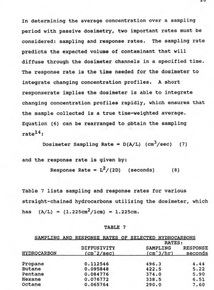
In determining the average concentration over a sampling
period with passive dosimetry, two important rates must be
considered: sampling and response rates. The sampling rate
predicts the expected volume of contaminant that will
diffuse through the dosimeter channels in a specified time.
The response rate is the time needed for the dosimeter to
integrate changing concentration profiles. A short
responserate implies the dosimeter is able to integrate
changing concentration profiles rapidly, which ensures that
the sample collected is a true time-weighted average.
Equation (6) can be rearranged to pbtain the sampling
ratel4.
Dosimeter Sampling Rate - D(A/L) (cm^/sec) (7)
and the response rate is given by:
Response Rate = L^/(2D) (seconds) (8)
Table 7 lists sampling and response rates for various
straight-chained hydrocarbons utilizing the dosimeter, which
has (A/L) = (1.225cmVlcm) = 1.225cm.
TABLE 7
SAMPLING AND RESPONSE RATES OF SELECTED HYDROCARBONS
RATES:
DIFFUSIVITY SAMPLING RESPONSE
HYDROCARBON_________fcro"2/sec)__________fcm'3/hr) seconds
Propane 0.112546
Butane 0.095848 Pentane 0.084776 Hexane 0.076772 Octane 0.065764
496.3 4.44
422.5 5.22
374.0 5.90
338.5 6.51
The sampling rate determined by this dosimeter design
ensures that sufficient air is sampled to detect a leak in
the vicinity of the dosimeter. The extremely short response
period guarantees that an average concentration over the
sampling period will be obtained, especially since the
ambient soil concentration is not expected to vary
significantly over the sampling period.
It is inaccurate, though, to assume the concentration at the
face of the dosimeter will be that of the ambient
concentration, and that the concentration in the
dosimeterwill be kept at zero. The concentration at the
face of the dosimeter, C^, will not always be the same as
the ambient soil concentration, Cg, because the air is
stagnant and re-equilibration may be hindered by certain
soil types or conditions (clay, moist soil). Since the
concentration gradient is the driving force behind getting
hydrocarbon(s) into the dosimeter, a decreased concentration
at the face will cause there to be a reduction in the
concentration gradient, and therefore a reduction in the
driving force. The assumption that Cq=0 can also be
challenged; although the chromate reduction reaction
proceeds rapidly, it is not instantaneous. This higher
actual concentration in the powder, Cp, from that expected
(Cq=0) , also seirves to decrease the effective driving force.
Since the ambient concentration measured will be slightly
concentration in the dosimeter slightly greater than zero
(Cp>0), there is a smaller concentration gradient and
thereby a smaller driving force for diffusion. This is shown graphically in Figure 5. The smaller actual drivingforce will cause the dosimeter to read low; concentrations obtained are less than the actual concentration. This
situation could be most detrimental at extremely low
concentrations, where the driving force is already very low,
and any further reduction could nearly eliminate the chance
of diffusion and thus detection.
FIGURE 5
DIFFUSION THEORY VIOLATIONS
CHROIiATE
POWDER
DRIVING FORCE FOR DIFFUSION IS Ca-Co
DOSIMETER POWDER HC CONC. IS Co
diffusion channel
SOIL VAPOR HC CONC. IS Ca
diffusion channel
Ca-Cf CHROMATE
POWDER
DRIVING FORCE FOR Cp DIFFUSION DECREASED Co
HC CONC. IN SOIL GAS NEAR DOSIMETER HAS
BEEN
DEPLEATED
IV. PRELIMINARY INVESTIGATIONS
A. Field
Field testing of the dosimeter and colorimetric chromate powder was done at Pope Air Force Base near Fayetteville, NC. Pope AFB was selected because it is a site of known contamination, and is well documented by previous
investigation^^. A preliminary site visit was conducted to
establish a sampling protocol, upon which further laboratory
analysis would be based.
1. Field Site Description
The Pope AFB fire training area is a sand field
approximately 500 feet long and 400 feet wide, and is shown in Figure 6. A "pit" about one foot deep and one hundred feet in diameter, surrounded by a restraining wall of sand
(about 3 feet high), is in the center of the field. In the pit are some large metal garbage dumpsters and three nozzles through which jet fuel (JP4) can be pumped.
During fire training practice, an average of 600 gallons of
31
FIGURE 6
POPE AFB SITE PHOTOS
Bi^^fl^^H^^^^^^u^ t /j^i^ jjflttMflRWi.
-ͣ
ji^^w^^j^n^^iip^^^^
,-/ ͣ
-ͣ'ͣ^*m^*:
- **'Jfj|^^^^^^^W
T „
-
1-.
•
THE POPE AFB FIRE TRAINING SITE.-"*
"»
» '
J
"THE PIT", WHICH IS PUMPED FULL OF FUEL DURING FIRE TRAINING
EXERCISES. IT IS PRESENTLY FILLED WITH WATER AFTER MANY DAYS
OF HEAVY RAINS.
resulting fire is extinguished as a fire-fighting drill-^^.
This has occurred 3-4 times per month for more than twenty
years. There is no liner in the pit to prevent the JP4 from
soaking into the ground, and over the years an enormous amount of fuel has contaminated the soil and groundwater.
2. Field Sampling Procedure
During the first visit to Pope AFB, the following sampling protocol was developed and established: A 20-inch deep hole
was dug with a 6-inch diameter post hole digger. This depth was chosen for two reasons. Firsts it is the depth at which previous soil vapor hydrocarbon concentration data had been obtained, allowing for comparison of results. Second, the groundwater level is often as high as 25-inches below the surface; the 20-inch level would prevent samples from being ruined by groundwater intrusion. The soil extracted from the sampling hole was placed around the mouth of the hole in the order removed. Accurate characterization of the soil at various depths could then be made.
The dosimeter was prepared by putting a 10-micron thick
membrane over the diffusion channels, and adding 1 gram of pre-weighed chromate powder. One gram of chromate powder
filled the well, and provided sufficient mass to enable
color determination through the viewing window. A string was attached to the loop on the dosimeter to simplify
then placed "diffusion holes down" into the hole so that the
diffusion channels were against the undistubed soil. The
soil was replaced in the hole in approximately the same
fashion as before the disturbance. The field procedure is
presented pictorially and by a photograph and in Figures 7
and 8, respectively. The dosimeter remained in the sampling
hole (temporary monitoring well) for 5 hours. At the end of
the sampling period, it was removed, and the chromate powder
color examined.
Three separate locations were tested during the preliminary
site assessment, all between 100-150 feet west (down
gradient) of the edge of the pit. The powder in two of the
three dosimeters had turned completely green, and a distinct
color change was evident in the third. Since the dosimeters
had completely reacted in the 5-hour sampling time, a
shorter sampling time could be used. After further
experimentation, a sampling period of three hours was
decided upon; this would enable three separate runs per day,
and would still be long enough to allow the powder to react
in a moderately concentrated environment.
B. Laboratory Trials
"^5^
34 FIGURE 7
DOSIMETER FIELD APPLICATION PHOTO
DOSIMETER IN SAMPLING HOLE. NOTE VIEWING WINDOW IS UP,
AND DIFFUSION CHANNELS ARE ON THE BOTTOM. STRING
SHOULD BE KEPT OUT FOR EASY (AND GUARANTEED!) REMOVAL.
•
pn^i^smswsmsaswsifiswsm
FIELD SAMPLING PROCEDURE
^S^^
GROUND LEVELSTEP 1 - DIG HOLE TO DESIRED
DEPTH, PLACING SOIL AROUND MOUTH
OF HOLE IN ORDER REMOVED
RETRIEVAL STRING KEPT OUT
STEP 2 - PLACE DOSIMETER INTO WELL WITH HOLES DOWN (VIEWING WINDOW UP)
BE SURE STRING IS KEPT ON GROUND SURFACE AND NOT BURRIED
,-,»•ͣ•••••ͣͣ•••ͣͣ•ͣͣ•ͣ I
1 * II ^
^RETRIEVAL STRING
STEP 3 - REPLACE DIRT IN REVERSE ORDER
OF REMOVAL. LEAVE IN PLACE FOR
EXPOSURE PERIOD.. REMOVE BY TUGGING ON STRING OR DIGGING OUT. RECORD COLOR
holistic. Depending on the length of time, the
concentration, and the type of hydrocarbon to which the
chromate powder is introduced, a gradient of color change is
evident. The color goes from an initial canary yellow to a
darker yellow, then into an olive green which lightens into
a mint green color. Lab experiments to determine the extent
of color change after exposure of the dosimeters to various
concentrations of hydrocarbons for 3-hour time intervals (to
be consistent with field protocol) were developed.
1. Procedure
To examine the extent of color change, the following
procedure was employed. One gram of colorimetric chromate
powder was measured out and put into the dosimeter. The
viewing window was put in place, and the top screwed on.
The dosimeter was placed in a 5.5L desiccator, and the lid
sealed by high vacuum grease. The following equation was
then used to determine the amount of liquid hydrocarbon to
be injected into the desiccator to obtain a desired
hydrocarbon vapor concentration (concentrations were
determined on a volume/volume basis as microliters
hydrocarbon per liter air).
V(uL) = C * P * f5.5) * M (9)
d * R * T * 10-^
Where: V = Liquid hydrocarbon volume, microliters
C = Concentration of HC desired, ppmV
P/RT = 1/Molar volume of gas (24.45 at STP)
5.5 = Volume of desiccator in liters
M = Molecular weight of liquid (g/mole)
The liquid hydrocabon was injected into the desiccator
(vapor pressures of the hydrocarbons injected were all high
enough to ensure that all of the liquid would volatilize
within a few minutes). The desiccator injection ports were
sealed immediately after the injection, and the dosimeter
was exposed to the hydrocarbon vapor for a predetermined
length of time. Prior to removal of the dosimeter at the
end of the sampling time, fresh air was blown into the
desiccator so that the hydrocarbon-containing air was forced
into a hood. Figures 9 and 10 depict this procedure.
2. Recording Color
A system of recording the color of the powder was also
necessary, and crayons were the method of choice. Five
distinct stages of powder color were used to classify extent
of color change and reaction. The initial powder is a lemon
yellow color which turns green when reduced by hydrocarbons.
The color gradient between yellow and green is caused by
some granules of chromate powder having been reduced to
green, while others remain yellow. The five numerical,
descriptive stages are given in Table 8. Figure 11 presents
these five stages of color development visually, and
specifies which crayons are used to make each specific
FIGURE 9
LABORATORY PROCEDURE
fl---ft
TT TT
STEP 1 - PLACE DOSIMETER IN SEALED DESICCATOR
STEP 2 - INJECT DESIRED AMOUNT OF
LIQUID HYDROCARBON (i.e. OCTANE)
INTO DESICCATOR. LEAVE THERE FOR PREDETERMINED AMOUNT OF TIME.
fl-c~
V
AIR BLOWN IN
^ͣͣͣͣ•ͣ'•ͣ'•ͣͣ•.*i.*i.*..*. *!>.••'. '••w Tn
>ͣͣ<...ͣͣͣͣ Vfii'ii ͣ'•••ͣ•.•.•. X HOOD
STEP 3 - BLOW CONTAMINATED AIR
INTO HOOD BEFORE REMOVING
DOSIMETER
m
FIGURE 10
LABORATORY PROCEDURE PHOTOS
4»
«•
n-Pentane
INJECTION OF LIQUID HYDROCARBON INTO DESICCATOR
CONTAINING DOSIMETER.
r
SEALED DESICCATOR, EXPOSING DOSIMETER TO
FIGURE 1 1
COLOR PRESENTATION
UNREACTED
YELLOW---FULLY REACTED ---ͨ GREEN
---4-COLOR NUMBERS:
0
f
COMBINATIONS OF CRAYONS (BY CRAYOLA CRAYON NAME) USED TO
MAKE THE COLORS ARE GIVEN BELOW. THE FIRST COLOR LISTED IS
THE BASE COLOR, THE SECOND COLOR IS THE TOP COLOR. ALL COLOR
COMBINATIONS WERE THEN COVERED WITH WHITE, SO AS TO BLEND
COLORS AND MAKE THEN APPEAR MORE UNIFORM (LIKE THE POWDER).
COLOR NUMBER:
0
1
2
3
4
CRAYON(S) USED:
YELLOW, MAIZE
MAIZE, OLIVE GREEN
OLIVE GREEN, MAIZE
SEA GREEN, SPRING GREEN
TABLE 8; General Color Descriptions
0: Unreacted yellow powder
1: yellow with a hint of green
2: half green, half yellow
3: mostly green with only a hint of yellow
4: All green, fully reacted.
3. Determination of a Hydrocarbon Standard
The first experiment involved injecting equal quantities
(260 microliters) of pentane or octane into a desiccator,
exposing the dosimeter for six different time periods, and
recording the color upon removal of the dosimeter from the
exposure environment. As can be seen by Figure 12, the
octane reacted at a faster rate than the pentane, even
though the actual concentration of octane (260 uL = 7120
ppmV) was lower than that of pentane (260 uL = 10030 ppmV).
This shows that higher molecular weight hydrocarbons (i.e.
octane) react more quickly and at lower concentrations than
lower molecular weight hydrocarbons (i.e. pentane). This
faster change is expected, as stoichiometry shows that the
higher the molecular weight of the hydrocarbon, the greater
the amount of chromate reduced per mole (from Table 4).
This variation among hydrocarbon species illustrated the
FIGURE 12
COLOR GENERATED BY OCTANE AND PENTANE EXPOSURES
OVERTIME
the standard to ensure its appearance in the soil gas near
leaking USTs, and because it is highly reactive with
chromate. Octane was chosen as the standard, as it is
representative of the higher molecular weight, more reactive
hydrocarbons present in the soil gas. An even higher
molecular weight hydrocarbon (C>8) was not chosen because
the literature suggests these species are more likely to
adsorb to the soil or be transported in groundwater due to
their lower vapor pressures (tendency not to volatilize).
Even though lower molecular weight hydrocarbons have higher
volatilities, these hydrocarbons do not reduce the chromate
as effectively on a per mole basis as does octane, as was
illustrated in Figure 12. Thus, even though more volatile,
the lower molecular weight HC's are not as sensitive as
octane. If the contaminant is gasoline (average molecular
weight "70 g/mole, similar to pentane) octane will cause the
color change to be indicative of a concentration higher than
the actual ambient concentration, a conservative approach
which is desirable in determination of environmental
V. RESULTS
This investigation into colorimetric passive dosimetry is
unusual, as it relies upon the qualitative interpretation of
color rather than upon a quantitative approach. At first,
determination of color may seem ambiguous and subjective;
the fist part of this section will show that colors can be
depicted and used in a quantitative manner. The second
part. Field Results, will show how color-concentration
values determined in the lab were then applied to assess the
Pope Air Force Base site.
A. Laboratory
Since a dosimeter measures the average contaminant
concentration over an exposure period, it was necessary to
calculate the average concentration of octane in the
desiccator over the three hour sampling period. Knowing the
average concentration would then allow for comparison of the
resultant color to the known average concentration (over a
specific sampling period).
The sampling rate of the dosimeter (with A/L =1.23 cm) for
octane (D = 0.065764 cm2/sec) is given in Table (7) as 290
concentration and is determined solely by dosimeter design
(A/L) and the diffusion coefficient, D, of octane in air.
The amount of hydrocarbon "sampled" (i.e. reacted) from the
desiccator after a given time can then be determined,
knowing the initial concentration. Assuming a complete,
instantaneous reduction of all hydrocarbons upon reaching
the chromate powder, the concentration (C^) after a given
time (t) can be calculated.
Mass Remaining = Init. mass - mass reacted
V Ct - VCq - RtCo (9)
Where: V = Volume of desiccator (5.5 L = 5500cc)
C^ = Concentration at time t (ppm)
Cq = Initial concentration (ppm)
R = Dosimeter sampling rate, cc/hour (290 cc/hr)
t = Time (hours)
So that:
Ct = Cq - [(RtCo)/V] (10)
Ct = Cq [ 1 - (Rt/V)] (11)
The average concentration over the time interval, C^yg, can
then be calculated by:
^avg = (^o + Ct)/2 (12)
Assuming an initial concentration of 7000 ppmV Octane was
injected into the desiccator, at the end of a three hour
sampling period, the expected octane concentration is (using
Equation 11):
The average concentration over that period is (Eqn. 12):
C = (7000 + 5983)/2 = 6646 ppitt
These formuli were applied to determine the average
hydrocarbon concentration in the desiccator over the entire
exposure period.
Having chosen octane as the standard hydrocarbon from which
color vs. concentration information would be obtained, three
separate experiments were run to determine the effect of
concentration on rate of color development over time. A
comparison between color obtained by exposing the dosimeter
to three different concentrations of octane (3560, 7210, and
14240 ppmV) for different sampling periods was made, and the
results are presented in Figure 13. As expected, the greater the concentration of octane, the faster and more
extensive the color change. Color change also progressed
with time of exposure.
Theoretically, all the hydrocarbons that reach the powder in
the dosimeter will react, thereby providing a measure of the
total amount of hydrocarbons sampled. This amount (grams,
ppm, etc.) can then be divided by the length of exposure
(hours, days, etc.) to determine the average concentration
COLORS FROM EXPOSURES TO VARYING
OCTANE CONCENTRATIONS AND TIMES
TIME (hairs)
the mass of hydrocarbon collected as:
M = (DCgjAt)/L (5)
Where: M = mass (grams) of contaminant collected, or in this case, reacted with the chromate
(expressed as extent of color change) D = Diffusion coefficient for the particular
contaminant gas (cm^/sec)
Ca = Ambient contaminant concentration (g/cm"^) A = diffusional area of dosimeter (cm^)
t = time exposed (sec)
L = Length of dosimeter diffusion channels, cm
The extent of color change (from yellow to green) is
directly related to the amount of hydrocarbon (M) which has reacted with the chromate. The greener the color, the
greater the amount (M) of hydrocarbon that has reduced the
chromate in the dosimeter. If the extent of color change for
two different samples is the same, it follows that the amount of hydrocarbon reacted, M, must also be the same.
Hence, since the M values are equivalent, and knowing M =
(DC^At)/L, an equation relating the two samples can be
established (where the subscripts denote samples 1 and 2,
respectively).
(Dl*Cal*Al*ti)/Li = (D2*Ca2*A2*t2)/L2 (14)
Since D, A, and L are fixed for a given dosimeter design and
Thus, the (concentration * time) value for samples of the
same color must be equal. The concept of ppm*hours is
hereby introduced.
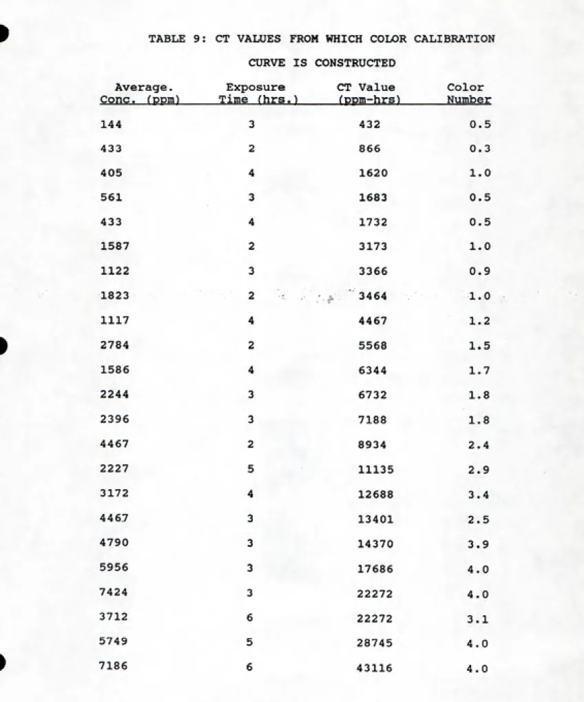
Given this concept, laboratory experiments were conducted to
determine the color of various ppm-hours, which becomes the
calibration curve for a given chromate powder strength,
dosimeter and standard HC. Table 9 lists the various
concentrations, times, and CT (concentration*time) values
for all points plotted in Figure 14. A best-fit line can be
drawn through the data, and,used as the calibration curve.
When a sample is taken in the field, the concentration can
be determined from the calibration curve (color vs.
ppm-hours. Figure 14). The field sample color is matched to the
appropriate color on the y-axis. Moving horizontally to the
calibration curve, the concentration*time value for that
color can be determined, which can then be divided by the
known exposure time to yield the average concentration. The
unit of ppm-hours is the fundamental value to which color is
compared to determine concentration.
Although octane is used as the standard to which the
contaminant(s) are compared, conversion from ppm as Octane
to ppm of a particular hydrocarbon can easily be made. For
TABLE 9: CT VALUES FROM WHICH COLOR C?
CURVE IS CONSTRUCTED
iLIBRATIOh
Average. Cone. fDDm)
Exposure CT Value Time (hrs.> (ppm-hrs)
Color
Number
144 3 432 0.5
433 2 866 0.3
405 4 1620 1.0
561 3 1683 0.5
433 4 1732 0.5
1587 2 3173 1.0
1122 3 3366 0.9
1823
2 :"'-i.
ͣ
;.•
ͣ
;;^^:::'"''3464' :'
ͣ
1.01117 4 4467 1.2
2784 2 5568 1.5
1586 4 6344 1.7
2244 3 6732 1.8
2396 3 7188 1.8
4467 2 8934 2.4
2227 5 11135 2.9
3172 4 12688 3.4
4467 3 13401 2.5
4790 3 14370 3.9
5956 3 17686 4.0
7424 3 22272 4.0
3712 6 22272 3.1
5749 5 28745 4.0
FIGURE 14
DOSIMETER AND POWDER CALIBRATION CURVE
COLOR VS. CONCENTRATION * TIME VALUES
(CT COMBINATIONS LISTED IN TABLE 9)
4
a.a
->^a
a
->^a
2.S -1
>6^ D
2
-t ͣ
^ a Best fit line
l^-^
X
1 H D
y
o.a H D
y
o -T 1 1 \ " 1 1 1 1 1 1 ... 1 ͣ...r...I 1 1
C 2 4 6 & 10 12 14 CTho uscsrid si
comes from a leaking gasoline tank, one can make the
assumptions and calculations listed in Table 10 to determine approximate ppm gasoline:
TABLE 10
CONVERSION OF PPM AS OCTANE TO HYDROCARBON-SPECIFIC CONCENTRATIONS
1. The stoichiometric equations of Table 5 show that 1 mole of octane reduces 8.33 moles chromate.
2. The average molecular weight of gasoline is 70 g/mole, similar to pentane (72.15 g/mole); assume the gasoline will react similarly to pentane.
3. Table 5 shows that 1 mole of pentane reduces 5.33
moles chromate.
4. To convert the concentration as octane to the
concentration of a particular hydrocarbon (if it is a complex mixture of many hydrocarbons, assume it acts as one of the straight-chain hydrocarbons of Table 4):
a) divide the amount of chromate reduced by the known hydrocarbon (i.e. gasoline or pentane) by the amount of chromate reduced by octane (8.33 moles chroraate/mole octane)
b) multiply this number (the correction factor) by the ppm as octane concentration obtained from the
calibration curve
c) the result is the hydrocarbon specific concentration.
5. Moles chrome reduced by gasoline (pentane)/moles reduced by octane = (5.33)/(8.33) - 0.64
6. If results indicated the soil vapor concentration was
100 ppm as octane, then the actual concentration of the
contaminant, if known to be gasoline (or pentane) is
100 * (0.64) = 64 ppm gasoline.
7. The correction factors for the hydrocarbons in Table 4
TABLE 11
Conversion Factors to Multiply PPM as Octane by to Obtain
Hydrocarbon Specific Concentrations
Propane 0.40
Butane 0.52
Pentane (Gasoline) 0.64
Hexane (Jet Fuel) 0.76
Octane 1.00
The colorimetric powder and calibation curve express total
hydrocarbon concentration as ppmV Octane. The issue of
total hydrocarbon (HC) measurement vs. environmental
. 18
contamination is ongoing. According to Eisenberg et. al.-^°,
regulatory agencies have not addressed the issue of total
fuel hydrocarbon analysis. Virtually no data exist on the
relationship between specific chemicals (i.e. xylene,
benzene, toluene, octane) and total hydrocarbon
concentration in environmental samples. A decision-making
procedure is in use in the San Francisco Bay area, which states that if total HC analyses indicate that if
concentrations greater than 100 ppm are present, the case is
classified as a "Fuel Leak Site" ^^. This concentration is
determined by measuring certain constituents via EPA protocol, and extrapolating to a total HC concentration.
McNerney uses 500 ppm total hydrocarbons as an alarm trigger
point^^. He claims that background levels from minor spills
concentrations to soar to 13,000 ppm total HCs, and common
background levels are often a few hundred ppm without any leaks. These high concentrations are caused by spillage and improper fuel handling over the years, which has slightly
contaminated the backfill of many tank beds.
B. FIELD RESULTS
The fire training area at Pope AFB near Fayetteville, NC is
the site where field studies were done. The purpose of the
field investigations was twofold: to quantify the extent of
contamination, and to compare the results obtained using the colorimetric dosimeter to previously documented soil HC
concentration studies. To thoroughly sample the area around
the pit, a "bullseye" of sample locations was made. This involved sampling at 50 foot intervals in a direct line away
from the pit in the major compass directions (N, NE, E,
etc) .
Sampling was executed in the same manner as described in
detail in the Preliminary Field Section; a sample location was selected, a 20-inch deep hole dug, the dosimeter placed
in the hole (with diffusion channels down), and the soil replaced in the hole. At the end of the three hour sampling period, the powder was carefully examined, removed, and
placed into a clean, labeled vial. The color was recorded immediately using crayons and the numerical (0 to 4)
dosimeter was then brushed off and cleaned, the membrane replaced, fresh (preweighed) powder added, and the dosimeter
placed into a new hole. This procedure was repeated for all
three dosimeters for up to three runs each (a step-by-Step Field Procedure is found in Appendix B). All vital
information on daily site sample locations, resultant powder color, general site conditions (weather, rainfall,
groundwater level, etc.) and hole specific data (type(s) of
oil, smell of JP4) was recorded and is found in Appendix C.
A total of nine trips to Pope AFB were made between May 2 and August 18, 1989. Thirty-four (34) locations were sampled once, and four of these sites were sampled twice because of some type of sampling problem or extraneous circumstance during the initial run. A maximum of nine
locations could be sampled in one day. Colors of the powder
from each of these sites was recorded. These color results
were then compared to the calibration curve and quantified as ppmV octane. Sampling location, date sampled (and repeat sample if applicable), and soil gas total hydrocarbon
concentration (in ppmV as octane) are presented in Table 12.
These concentrations were measured over a three month
period, and are therefore intended to be indicative only of
general concentration trends. A concentration contour map
of the Pope site was then developed with these data, and is
TABLE 12; FIELD SAMPLING HC CONCENTRATION RESULTS
LOCATION DATE RESULT fPPM HCs AS OCTANES REPEAT RESULT N50 NlOO N150 N200 NWlOO NW150 NW250 NW300 NW350 NW300S50 NW3 00N25 NW300N25W25 W150 W200 W250 W350 W400 SW25 SW50 SWIOO SW150 SW100W100N25 SWIOOWIOO SW100W150 SW100W50 S50 SlOO SE2 5 SE50 E25 E50 ElOO NE25 NE50 AMBIENT @ W150 7/28/89 7/20/89 7/28/89 7/28/89 7/14/89 7/14/89 7/28/89 8/18/89 8/18/89 8/19/89 8/19/89/ 8/19/89 7/14/89 7/20/89 7/20/89 7/20/89 7/20/89 8/18/89 7/28/89 7/20/89 8/19/89 8/19/89 8/19/89 8/19/89 8/19/89 8/18/89 7/20/89 8/18/89 8/18/89 8/18/89 7/28/89 7/20/89 8/18/89 7/28/89 8/19/89 4100 4670 2330 < 585 >4670 3500 < 585 < 585 < 585 1170 1170 >4670 >4670 3500 >4670 >4670 < 585 NCC 3500 2330 4095 >4670 1175 <585 2330 < 585 < 585 < 585 < 585 NCC 2330 < 585 ~1000 (2.5-HR ONLY) 5-HR SAMPLE 5-HR SAMPLE SEEPAGE 7/28/89 7/28/89 <585 4095
8/18/89 >4670
5-HR SAMPLE
SEEPAGE
7/20/89 >4670
15 MIN. ONLY, ASSUME TO BE>4670
LOCATION: Measured as distance from edge of pit in feet in compass direction indicated.
NCC: No color change (less than _150ppm)
NOTE: All samples on August 19th read somewhat higher than normal due to fire training and filling of the pit the previous day; even
ambient air was high due to fumes from pit. Strong smell of fuel
POPE AFB SOIL VAPOR HYDROCARBON CONCENTRATIONS
AS GIVEN BY NAPFEL UTILIZING THE COLORIMETRIC PASSIVE DOSIMETER
(IN PPM TOTAL HYDROCARBONS AS OCTANE)
'+ͣ INDICATES SAMPLE LOCATION SITE
CONTOUR INTERVAL 500 PPM
30C500
+ +
200
% *
m
8
0(200 100
+ + +
4000 4000
+ +
99
3
NORTH
A
4'UOO
+
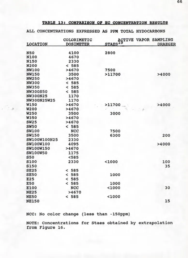
Soil gas total hydrocarbon concentrations were also measured
by Staes^^ between January and March, 1989. Staes also
developed total HC concentration contour curves for the Pope AFB site, presented in Figure 16. The colorimetric
dosimeter results show the same general concentrations and extent of contamination as those obtained by Staes.
Although some of the concentration values obtained with the
dosimeter were lower than those of Staes, the general trends were very similar. Both the colorimetric dosimeter method and Staes' results (active vapor sampling fom permanent samplin wells with a vapor pump and gas chromatography analysis) show a pocket of very high soil gas hydrocarbon concentration approximately 250 feet due west of the pit. Both methods indicate the high concentrations to be above 4000 ppm total hydrocarbons, and agree that contamination east of the pit (upgradient) is minimal. Differences in the concentrations measured are most likely due to the
differences in sampling conditions; heavy rainfall, recent fire training practices, and the time period samples were
taken (Staes in January-March 1989, Napfel in May-August, 1989) may all contribute to the varying soil concentrations measured. Entrained ambient air in the replaced soil above
POPE AFB SOIL VAPOR HYDROCARBON CONCENTRATIONS
AS GIVEN BY ED STAES
(IN mg/M^ AS TOTAL HYDROCARBONS)
• INDICATES SAMPLE LOCATION SITE
Aldlsh Rd
POPE AIR FORCE BASE
NORTH CAROLINA
FIRE TRAINING AREA «4
Leachate
"h
Leachate
VAPOR-PHASE TOTAL HYDROCARBON CONCENTRATIONS
.3
(mg/m )
contour Interval 10.000 mg/m^
March. 1989
NORtH
100-Scale:
• Sample Location
CONVERSION OF mq/M^ TO PPri:
I mg/M3 = (PPM) • (HC MOLECULAR WGT./24.45)
mg/N^ (STAES) PPM (NAPFEL)
5000 1070
15000 3210
25000 5350
35000 7490
45000 9630
sampling times been long enough to allow for
re-equilibration to ambient soil concentrations, readings would
most likely have been higher and more comparable.
Soil HC concentration data were also obtained by active vapor sampling of permanent wells by colorimetric Draeger tubes. The Draeger tubes worked on the same principle as the colorimetric dosimeter; color change from yellow/orange to green by reduction of chromate upon exposure to
hydrocarbons. A schematic representation of a Draeer Tube is given in Figure 17.
CONCENTRATIONS WDICATED W PPM TOTAL HYDROCARBONS
>I
7 MM13 CM.
DRAEGER TUBE
(TO SCALE)
FIGURE 17
Draeger tubes are sealed glass tubes, approximately 5-inches long and 0.25 inches in diameter. The tube contains a
of tube into a manual vapor pump, and the other end into the
environment to be sampled. The procedure at Pope AFB
involved utilizing the permanent vapor sampling wells at the
site (Figures 18 and 19), the same as those employed by
Staes. A piece of tubing connected the Draeger tube with a
sampling port that pulled vapor from 20-inches below ground
level. Draeger directs that 200 cc of air be drawn through
the tube. The granular material in the tube changes from
orange to green when exposed to hydrocarbons. The granules
at the monitoring end of the tube are the first to react
with any hydrocarbons that enter the tube. When these
chromate granules have been reduced, the air containing
hydrocarbons proceeds further down the tube, reducing
additional chromate granules along the way. The extent of
color migration has been calibrated by Draeger, and is
presented as ppm Total Hydrocarbons.
The Draeger tubes were designed to measure between 30 and
1000 ppm total hydrocarbons (HC's), although explanation of
how total HC's is calculated was not given (i.e. total HC's
as octane, etc.). The distance between divisions differed
significantly, being large on the low (30-300ppm) end of the
scale, and very close together on the high end (Figure 17).
Because divisions between 400 and 1000 ppm are so close
together, differentiation is difficult and could easily