1
EXAMINING NORTH CAROLINA’S COMPENSATORY WETLAND
MITIGATION PROGRAM FROM THE PERSPECTIVES OF LAND USE
PLANNING AND SOCIAL EQUITY
by
AUDREY STEWART
A Master’s Project submitted to the faculty
of the University of North Carolina at Chapel Hill
in partial fulfillment of the requirements
for the degree of Master of Regional Planning
in the Department of City and Regional Planning.
Chapel Hill
2009
Approved by:
___________________________
2
A
BSTRACTNorth Carolina’s Ecosystem Enhancement Program (EEP) is responsible for providing the majority of
compensatory stream and wetland mitigation sites throughout the state, including all off-site mitigation
for the N.C. Department of Transportation. Two emerging criteria by which to assess the effectiveness of
mitigation efforts include whether the mitigation process promotes social equity, and whether stream
and wetland mitigation planning is coordinated with other types of land use planning. The first part of
this study assesses the socioeconomic makeup of census tracts around impact sites in comparison to
mitigation sites using two-tailed paired t-tests. The second part of the study maps the location of the
EEP’s accumulated advance mitigation sites in comparison to urban growth indicators by watershed
around the state. The study finds that systematic socioeconomic disparities exist between communities
that lose and gain streams and wetlands through the compensatory mitigation process. Streams and
wetlands are systematically relocated from more advantaged to less advantaged communities.
Communities near impact sites, as compared to those around mitigation sites, have higher total
populations and population densities, higher percentages of whites and lower percentages of blacks and
Hispanics, higher levels of education, lower poverty rates, higher median incomes, and higher median
homes values. This finding warrants further consideration in both research and also state-level
environmental policy. Additionally, growth indicators such as population growth rates and population
growth projections do not significantly correlate with the amount of advance mitigation acquired by the
EEP by watershed, implying that growth indicators are not effectively incorporated in the mitigation
process. Thus, the EEP, the NC DOT and the Army Corps of Engineers have an opportunity to improve
the efficiency of mitigation by more proactively and formally incorporating growth indicators and
3
A
CKNOWLEDGEMENTSI am grateful for the guidance and support of a number of individuals without whom I could not have
completed this research. First and foremost, thank you to my advisor, Todd BenDor, who, as a leading
expert in the field of wetland mitigation analysis, provided the impetus for my research topic, suggested
analytical methods, directed me to relevant literature, and offered patient suggestions for improvement
along the way, not to mention providing a statewide data set on impact and mitigation sites that I used
for half of my analysis. Thank you to Joel Sholtes for his role in compiling the statewide dataset on
impact and mitigation sites. Thank you to Jennifer Doty, Catherine Zimmer and the helpful staff at Odum
for their assistance with GIS and STATA. Finally, thank you to my immediate family members, who, in
their loving ways, consistently motivated me to complete this project through a variety of cajoling and
4
I
NTRODUCTIONIn the past few years, North Carolina’s Ecosystem Enhancement Program (EEP) has been hailed as a
cost-effective and innovative statewide approach for preserving and restoring stream and wetland
ecosystems (D’Ignacio, 2005; Gilmore, 2005; EEP, 2009). Its approach to coordinating compensatory
mitigation is unique in that the government agency is responsible for providing the majority of
mitigation sites throughout the state, including all off-site stream and wetland mitigation for the
Department of Transportation (NC DOT). The recipient of numerous “innovative government” awards,
EEP has even been suggested as a model for other regions (D’Ignacio, 2005; EEP, 2009). While the
program has been analyzed from the standpoints of bureaucratic and cost efficiency (Engler, 2005; DYE,
2007) and watershed health (BenDor et al, 2009), comprehensive studies of the EEP from the
perspective of social equity and in relationship to urban growth across the state have, until now, been
lacking.
Since the passage of the Clean Water Act in 1972, which mandated mitigation for impacts to wetlands,
the key criterion for wetland mitigation policies across the country has been to achieve the underlying
goal of “no net loss” of streams and wetlands (National Academy of Science, 2001; Gutrich, 2004). While
theoretically no net loss implies no loss of ecosystem function, in practice it has often been applied in
terms of acreage and been measured by a simple ratio of acres of mitigation to acres of impact. Much of
the literature on wetland mitigation examines whether no net loss is achieved from an ecological
standpoint. For example, BenDor and Brozovic (2007) found that in the Chicago region, counties which
had adopted regulations based on municipal boundaries were more likely to see shifts in wetlands from
one watershed to another; while these counties maintained total wetland acreage, the mitigation
process may have created net change in ecosystem functionality. In North Carolina, BenDor et.al. (2009)
found that while most wetland impacts are mitigated within the same 8-digit HUC watershed (as
required by state legislation), a significant amount of cross-watershed relocation of wetlands does
occur.
While numerous studies focus on the no net loss criterion as a measure of mitigation success, fewer look
at relationships between wetlands and human communities. Those that do generally consider issues
such as how to determine the economic and social value of wetlands (e.g. Reynolds and Regaldo, 2002;
Manuel, 2003; Boyer and Polasky, 2004). Recently, social equity has emerged in the literature as another
5
wetland mitigation and social equity has found that, when considering a smaller geographic scale suchas census tract or zip code, there are notable socioeconomic disparities between populations in areas of
wetland loss and those in areas of wetland mitigation offset sites (Ruhl and Salzman, 2006; BenDor et.
al., 2007; BenDor et. al. 2008). However, this criterion has played no factor in wetland regulations to
date and has not been previously studied in the North Carolina context.
Additionally, there is growing awareness from regulators and practitioners about the importance of
linking wetland preservation efforts to the broader context of land use planning and urban growth. This
is evident, for example, in North Carolina’s Targetted Local Watershed planning program, in which local
water resource planners consider growth projections as part of the process to identify priority areas for
stream and wetland restoration and preservation (EEP, 2007). However, the extent to which mitigation
activities and urban growth are coordinated in practice has not been widely explored in either the
planning or ecology literature. Given that larger amounts of wetland impacts would be expected in more
rapidly urbanizing areas, it would make sense for the EEP to link their mitigation acquisition programs
with such land use considerations. In North Carolina, the water resource planning procedures that
influence the selection of EEP mitigation sites do take urbanization and land use projections into
account through the EEP’s Local Watershed Planning Process (New Hanover County, 2002; EEP, 2009).
However, no studies have considered the extent to which the EEP process for mitigation acquisition
relates to levels of urban growth across the state.
Given the set of issues described above, this paper seeks to answer two questions regarding North
Carolina’s statewide compensatory mitigation program. First, are there any socioeconomic disparities
between the populations surrounding impact sites and those surrounding mitigation sites? Second, do
watersheds in which the EEP has acquired advance mitigation sites spatially correspond with areas of
high needs (i.e. areas with high levels of urban growth and thus more wetland impacts from
development)? The first question is addressed in this study by an examination of state-level spatial data
on the location of historic impact and mitigation sites in relation to socioeconomic indicators from the
US census developed by BenDor et al. (2009). The second is addressed by looking at statewide data on
advance mitigation acquisition by the EEP in relation to growth indicators across the state developed by
DYE (2007). The results of the investigation have implications for wetland mitigation policy in North
Carolina, and contribute to academic and applied discussions on both links between land use planning,
transportation planning and natural resource planning, as well as emerging discussions on links between
6
B
ACKGROUNDWetland Ecosystem Services and US Wetland Regulations
The ecosystem functions of wetlands may include processes like hydrologic flux and storage, biological
productivity, biogeochemical cycling and storage, decomposition, wildlife habitat and others (e.g.
Richardson, 1994 as cited in Engler, 2005). From these functions, society receives services such as flood
control, water purification, recreation opportunities, open space and biological diversity (Manuel, 2003;
Ewel, 1997). These ecosystem services provide value to society, which, in recent years, an increasing
number of market-oriented initiatives around the globe have attempted to capture economically
(Salzman, 2005). Several aspects of ecosystem services justify and necessitate government intervention
to help define markets; for example, the often non-exclusive nature of the benefits of ecosystem
services leads to large “free rider” potential, and without clearly defined buyers and sellers, transaction
costs can be high (Salzman, 2005).
In the U.S., markets for wetland ecosystem services have largely been shaped by federal environmental
policy. To protect and allow for continued human access to such services, wetlands in the US have been
regulated by the federal government since passage of the Clean Water Act (CWA) in 1972. The CWA
provides for the use of regulatory and non-regulatory tools to restore and maintain “the chemical,
physical and biological integrity of the nation’s waters” (33 USC 1251). Some of the key tools dealing
with wetlands are provided in Sections 401 and 404, which establish requirements and procedures for a
permitting system regulating dredge and fill of wetlands and other US waters.
Under Section 404, developers applying for a permit must follow a multi-step process regarding wetland
impacts. First, avoid impacts if possible. If not possible, then loss or damage of wetlands must be
minimized (often achievable through site design). Finally, any unavoidable loss of wetland function or
acreage must be compensated through restoration, creation, enhancement or (in exceptional cases)
preservation of wetlands. This compensatory mitigation process requires a minimum 1:1 ratio of
mitigation to loss, often applied in terms of acreage, under the driving policy of no net loss (US EPA, no
date). Numerous difficulties arise in the quest for no net loss, such as how to measure the precise
values of services provided by two similar ecosystems each in a different geographic context (Salzman,
7
of mitigation require a more than one-to-one ratio of acreage in order for the mitigation to receive anappropriate number of mitigation credits (DYE, 2007).
Approaches to Wetland Mitigation
Approaches to compensatory wetland mitigation vary, and multiple types of compensation may occur
within a given region. BenDor et. al. (2007) identify three types of approaches for wetland mitigation. In
onsite or offsite “permittee-responsible mitigation,” the permit applicant (i.e. developer) directly carries
out mitigation. Alternatively, developers can pay a third party through mitigation banking (the purchase
of credits by developers from a bank of “pre-impact” restoration sites) or in-lieu-fee (ILF) programs
(payment into a government or not-for-profit pool of funds for future restoration activities). Initially
under CWA Section 404 legislation, the EPA and the Corps preferred on-site mitigation, but over time
off-site mitigation has become more accepted. This change has led to an increase in the creation and
sale of wetland mitigation credits throughout the US by private, third-party mitigation bankers and to
the rise of an ecosystem services market around wetlands in the U.S. (Salzman, 2005).
Ecosystem Enhancement Program History and Operations
In North Carolina, compensatory wetland mitigation is coordinated by a government agency called the
Environmental Enhancement Program (EEP). The EEP’s three primary goals are to identify high-quality,
cost-effective projects for watershed improvement and protection; to provide compensation for
unavoidable environmental impacts from transportation-infrastructure and economic development; and
to carry out detailed watershed-planning and project-implementation efforts in North Carolina's
threatened or degraded watersheds (EEP, 2009). The four components of the EEP’s mitigation program
include the stream and wetland ILF which provides mitigation for all CWA Section 404, 401, and N.C.
Coastal Area Management Act permits excluding the NC DOT; the stream and wetland ILF for the NC
DOT, which receives advance funding by and exclusively provides off-site mitigation specifically for the
NC DOT; the Riparian Buffer ILF; and the Nutrient Offset ILF which provides nutrient reduction projects
primarily for activities related to development in the Neuse and Tar-Pamlico River Basins (DYE, 2007).
The EEP was created by a Memorandum of Agreement (MOA) between the NC Department of Natural
Resources (DENR), the US Army Corps of Engineers (Army Corps) and the NC Department of
8
to streamline mitigation needs of the NC DOT. When created, the EEP was structured to combineprovision of advance-mitigation for the NC DOT’s projects (the largest individual source of stream and
wetland impacts in the state; BenDor et al, 2009) with the ILF program formerly run by the WRP for
non-DOT mitigation needs (DYE Management Group, 2007; EEP 2009). Prior to establishment of the EEP, the
NC DOT sought approval from the Corps for each individual project, which increased project costs and
time. Given the high levels of population growth throughout the state by the late 1990s, a key tenet of
the EEP was to reduce the NC DOT’s project costs and lag time by providing “cumulative mitigation for
cumulative impacts” in a given watershed, rather than mitigate for individual projects (D’Ignacio et. al,
2005).
In order to determine where the majority of advance mitigation credits should be acquired, the EEP
largely relies on annual forecasts of future impacts from the NC DOT (EEP, 2008), and also considers
other permitted development (EEP, 2009) as further discussed below. The number of credits provided
by a given mitigation project is estimated through a dynamic feedback process between the EEP project
manager, project supervisor, and if necessary an alternative mitigation review team. Credits are
estimated in acres for wetlands and feet for streams, and are based on an in-house assessment, a
project feasibility study, and the restoration plan. The final credits for a given mitigation project are
recorded after that project is successfully completed (EEP, 2008).
Since its creation in 2003, the EEP has become the primary provider of mitigation credits for both public
and private entities across the state, including the NC DOT, other public agencies, and private
developers (BenDor et. al, 2009). Recently, however, North Carolina has taken steps to foster the private
market for wetland mitigation banking in the state with the passage of a General Assembly Bill in
August, 2008. The bill seeks to limit the ability of any Section 404 Permit Applicant other than the NC
DOT to utilize the EEP for compensatory mitigation. Instead, applicants other than the NC DOT are
encouraged to participate in a private wetland mitigation bank, and may only pay a fee to the EEP if the
permit is for a project in an 8-digit HUC watershed where no approved private mitigation bank is
operational (North Carolina General Assembly, 2008). Such legislation indicates ongoing interest on the
part of mitigators and policy-makers to continually assess and improve the efficiency and
cost-effectiveness of stream and wetland mitigation programs in North Carolina.
9
The EEP seeks to implement mitigation in concert with a “detailed watershed-planning process” thatlinks the mitigation process with overall plans for watershed improvement, protection, and open space
protection (EEP, 2009). Through its collaboration with the NC DOT and with water resource planners
working at the local-watershed and basin-wide scales, there are opportunities for land use and
urbanization issues to be taken into account in the mitigation site selection process, to the extent that
local watersheds with higher growth forecasts are considered priority locations for mitigation sites.
However, the EEP policies and procedures that guide mitigation at the state level do not specifically
mention incorporation of land use change, urban growth patterns or population projections in the
process by which mitigation sites are selected by the agency, instead emphasizing the role of the NC
DOT’s forecasts in determining mitigation needs (EEP, 2008). Thus while land use forecasts play a role in
the selection of mitigation sites within each 8-digit watershed, these projections do not necessarily
affect the number of predicted credits needed for any given watershed (further discussed below).
The NC DOT’s annual mitigation demand forecasts, which drive advanced mitigation planning, are based
on the DOT’s Transportation Improvement Program (TIP) (DYE, 2007), which is the NC DOT’s
regularly-updated plan for transportation projects throughout the state. The State TIP (STIP) includes a schedule
and funding information for the state’s transportation projects including highways, aviation,
enhancements, public transportation, rail, bicycle and pedestrians, and the Governor’s Highway Safety
Program (NC DOT, 2008). Metropolitan Planning Organizations (MPOs) throughout the state also
develop MTIPs for regional projects (NC DOT, 2008). The EEP uses the forecasts to determine the types,
locations and amount of mitigation needed. Depending on the needs, the EEP may satisfy requirements
through its own inventory, or by procuring addition units of mitigation through means including asset
transfer from the NC DOT; purchase of suitable mitigation from either private mitigation banks, private
land owners with High Quality Preservation, or Clean Water Management Trust Fund project grantees;
or developing new mitigation (DYE, 2007).
Although the NC DOT is making noted improvements in determining future demand, their projections
about upcoming transportation projects, and thus future mitigation needs, have “a certain amount of
volatility” according to DYE (2007). The priority and sequencing of projects may vary based on a number
of factors such as funding constraints, changes in policy-maker priorities, and unanticipated delays.
Thus, there is some lack of predictability in the NC DOT’s demand forecasts, which leads to uncertainty
in EEP’s mitigation process (DYE, 2007). Additionally, as the NC DOT learns from experience, the
10
project selection was dominated by a legislative priority to deliver on unfinished portions of theIntrastate Highways and Urban Loops program, as well as focus on other major expansion projects;
however, the 2004 Long-Range Transportation Plan noted that future project selection should focus on
meeting “certain technical and needs-based criteria” (NCDOT, 2004). Noted improvements in the
precision of NC DOT mitigation demand forecasting is attributed to growing levels of experience by NC
DOT staff, as well as increasing awareness about the cost impacts of incorrect estimates (DYE, 2007).
Given the large role that the NC DOT forecasting plays in the EEP site selection process, one aspect that
needs to be considered in understanding the links between mitigation site selection and urban
growth/land use planning is the extent to which such issues factor in to the NC DOT planning process.
The NC DOT outlines the long-range transportation investment strategy for North Carolina in its
Statewide Transportation Plan. North Carolina’s first statewide transportation plan was developed in
1995 and an updated version of the 25-year plan was published in 2004 and is revised approximately
every four years. The plan provides estimates of infrastructure needs including predictions for
maintenance, modernization and expansion. The NC DOT implements the long-range plan in part
through the TIP program, a seven-year blueprint for new transportation projects (NC DOT, 2004).
The NC DOT long-range transportation plan consists of a three-tiered approach to managing
infrastructure, including statewide, regional and sub-regional levels. The statewide Strategic Highway
Corridors program is a major component of all TIP projects, because while these roadways account for
about 7% of all road miles in the state, they carry about 45% of statewide traffic (NC DOT
Transformation Management Team, 2007). Priorities in determining strategic corridors include
connectivity between major activity centers and interstate highways, providing relief for interstates,
hurricane evacuation routes, and whether the route is part of other organized highway systems (NC
DOT, 2004). Highway preservation, modernization and expansion comprise about 93% of the NC DOT
budget (NC DOT, 2004), and the NC DOT manages more public highway miles than any other state
except Texas (NC DOT Transformation Management Team, 2007).
Considering that the emphasis of the statewide NC DOT program is on highway projects and the
priorities for Strategic Highway Corridor planning have little to do with urban growth and land use
concerns, it seems unlikely that urbanization and growth are directly represented in the NC DOT’s
forecasts to the EEP. Concerns about a general disconnect between transportation and land use
11
Highway Administration (FHA) report notes that transportation and land-use planning processes areoften not integrated in the U.S., in spite of the influences of development on transportation demand
and of transportation facilities on development location. This is generally a result of the different scales
of decision-making, with transportation project plans made at a regional scale while land-use planning
occurs locally (FHA, 2001). The relevance of this issue to the North Carolina context is indicated in a
report on the advisory sessions to the incoming State Governor; a variety of administrative changes are
suggested to decrease a noted disconnect between land use and transportation planning (University of
North Carolina at Chapel Hill School of Government, 2008).
A second process by which urban growth and land use considerations may be reflected in the acquisition
of mitigation sites by the EEP is through its local watershed planning process, which requires that the
EEP’s compensatory wetland mitigation be consistent with basin wide plans for restoration. This
includes coordinating with local watershed planning (14 digit HU). According to the EEP, local watershed
planning is a dynamic process that takes into account both quantitative data (including the NC DOT’s
forecasted mitigation needs as well as existing hydrology, habitat and land use) as well as local
community priorities as determined through a participatory stakeholder process (EEP, 2008). Estimated
mitigation needs can change on a month-to-month basis, meaning that the process of setting priorities
for mitigation requires a flexible approach (EEP, 2008). The EEP’s procedures state that the agency will
develop mitigation in watersheds in which it predicts needing mitigation in the “next few years.” The
EEP’s mitigation target tables are updated every six to eight weeks, and the acquisition objectives,
timelines and outreach methods are revised to reflect updated mitigation targets (EEP, 2008).
In order to coordinate its mitigation program with local watershed planning, and in concert with
basin-wide planning goals, the EEP identifies priority sites for restoration through a multi-step planning
process and then targets those sites as potential mitigation. In the first step, the EEP’s staff members
utilize GIS data, field tours and input from other water resource professionals to identify watersheds at
the 14-digit HU level that have both problems and assets. As part of this process, staff identifies major
functional stressors (Bryson and Leslie, 2009), which may include development pressure (projected
residential and commercial land use). The watersheds are ranked and those with the highest need and
opportunity become designated as “targeted local watershed” (TLW) – areas in which preservation,
restoration and enhancement projects would have the largest benefit. By 2008, just under 25% of all
12
The second step is to develop local watershed plans, which is informed by factors including the NC DOT’sactivities as well as other permitted impacts associated with other types of development. Again through
a dynamic process involving quantitative and qualitative factors such as GIS information and stakeholder
interest in each local watershed, focus areas for each local watershed are determined. The LWPs are
comprised of a Watershed Assessment Report discussing the major ecological functionality within the
targeted area, a Project Atlas with site-specific information about the most promising mitigation sites in
the study area, and a Watershed Management Plan containing policy and other recommendations to
address critical local watershed problems (EEP, 2009).
The final piece of the mitigation process involves the actual property or easement acquisition. Sites are
acquired in the 8-digit watersheds in which impacts are predicted, with priority placed on sites in
selected 14-digit TLWs. Using the Project Atlases, the EEP’s staff pursues project sites with high
potential; in theory these are sites where the EEP will be able to achieve the greatest ecological return
on investment from the standpoint of water quality, hydrology and habitat (EEP, 2009). Often the sites
are privately owned and the actual acquisition of an easement occurs through a series of property
transaction negotiations; thus, like with other land conservation transactions, implementation depends
in part on successful negotiations with land owners (DYE, 2007). At times, projects are also pursued
outside of TLWs, if the site offers substantial ecological benefits or would allow mitigation goals to be
met in a timelier manner (EEP, 2009).
In numerous LWPs, commercial and residential development was cited as one of the largest threats to
local water quality, because activities like channel modification, stream relocation, straightening and
dredging, which cause water quality impacts like increased storm water runoff and sediment, are
primarily associated with road-building or residential areas. Analysis completed during the creation of
local watershed plans considers factors such as projections for residential and commercial development
and anticipated increases in impervious surface cover. Some plans utilize future land-use projections
and scenarios to develop models for estimating non-point source pollutant and run-off loads for various
time-frames and under various management and regulatory conditions (e.g. EEP, 2007) or to develop of
watershed-wide and subcatchment-specific build out development models (e.g. New Hanover County,
2002). LWPs also generally include a list of recommendations for restoring or improving water quality.
The majority of these recommendations are site-specific, such as on-site BMPs, water-quality
monitoring, and habitat restoration and preservation. However, some recommendations also include
13
creation of comprehensive land use plans (EEP, 2007), thus providing an additional way by whichland-use and water resource planning are linked in practice.
A final way that land use considerations may be incorporated into local watershed planning is through
the inclusive stakeholder aspect of the process. Types of stakeholders representing urban growth
interests include regional Council of Governments (COGs), local elected officials from cities, towns and
counties, and landowners. They provide input through processes including informational exchange at
meetings, and representation on advisory committees (Bryson and Leslie, 2009). A contracted facilitator
is normally involved in the process, such as the regional COG or the North Carolina State University’s
Watershed Education for Communities & Officials program (EEP, 2008).
It is clear that land-use planning measures, such as population and development forecasting and
projected changes in impervious surface cover, are incorporated into TLW planning at the 14-digit
watershed level to identify local priorities for preservation and restoration. However, these indicators
are used generally from a reactive standpoint, in that development is considered a stressor to local
watershed health, rather than from a proactive standpoint in which future developed projections would
be used to determine advance mitigation needs. This approach mirrors much of the current literature
linking urban growth with wetlands, which primarily focuses on how urban development influences
ecology and water quality (e.g. Carpendo, 2007) but not how growth forecasting and land use planning
can be used to proactively plan for mitigation.
Additionally, there is no evident attempt by the EEP on a broader, landscape-level scale to coordinate
mitigation with rapidly-developing watersheds beyond considering already-permitted development .
The difference in scale at which targeted local watershed plans are created versus at which mitigation
must occur (i.e. 14 digit versus 8 digit watersheds) leaves room open for spatial mismatches between
watersheds that are rapidly growing and those that are gaining much mitigation. This may be true, for
example, when a 14-digit watershed is expected to undergo high levels of development but has little
opportunity for mitigation for reasons like lack of sites, or high property values, or land ownership
structures not well suited for purchase of easements by the EEP. In such a case, that particular 14-digit
watershed may not be prioritized for restoration as a TLW, and may create a situation in which
mitigation is needed at the 8-digit scale but is not accounted for in the local watershed plan and is thus
14
Wetland Mitigation and Social Equity
Over the past few decades, social equity or “environmental justice” has become an emerging criterion
by which to measure the success of solutions to environmental challenges. With the issuance of
Executive Order 12898 in 1994, President Clinton made environmental justice a national concern,
mandating that Federal agencies avoid causing any disproportionate public health or environmental
effects on low-income and minority populations (Clinton, 1994). The traditional environmental justice
perspective is based on the idea of preventing a disproportionate burden on disadvantaged populations
(Clinton, 1994) and the more recently-emerging view hold that disadvantaged communities should also
have fair access to environmental “goods” (e.g. Alkon, 2006). Several recent studies suggest that stream
and wetland relocation occurs as an unintended consequence of compensatory wetland mitigation
programs, raising the question of whether any disproportionate environmental or economic effects
accrue to certain populations and not others (Ruhl and Salzman 2006; BenDor et al 2007; BenDor et al
2009).
Evidence increasingly suggests that in spite of the “no net loss” clause governing wetland mitigation in
the US, mitigation programs do result in spatial relocation of streams and wetlands, with ecosystem
services being lost at impact sites and gained at mitigation sites. Several recent studies confirm that
compensatory mitigation programs result in a systematic loss of wetlands from urban or urbanizing
areas, while mitigation tends to occur in less densely populated areas (Ruhl and Salzman, 2006; BenDor
et al, 2007).
The spatial relocation of wetlands may have implications for social equity in a variety of ways. The
differences between the scales and boundaries of watersheds versus political jurisdictions and human
communities means that even with legal requirements for mitigating stream and wetland losses within
specific ecological boundaries (8 digit watersheds in North Carolina), any social impacts of relocation
beyond large-scale watershed-quality issues are not accounted for in mitigation policy. Further, many
benefits of wetlands are realized at a local level, including services with both direct and indirect “use
value.” Direct use-values of wetlands include water purification (such as a sewage treatment area),
wildlife harvesting, peat production, and low-impact transport, while indirect use values that have very
local benefits include flood control, storm protection, micro-climate stabilization, and shoreline
stabilization. The scale at which these benefits are realized differ from the scale at which wetland
15
such as ground water recharge and water filtration from pollutants (e.g. nitrogen, phosphates) (Boyerand Polaski, 2004).
In order to understand whether wetlands are considered an amenity and to understand their economic
value to local communities, a variety of methods have been employed. Studies looking at the market
and non-market values of wetlands find differing results, depending on factors like analytical methods,
location of wetland (e.g. urban or rural), type of wetland, and whether the studies look at market or
non-market value (e.g. Boyer and Polasky, 2004; Reynolds and Regaldo, 2002).
A review of non-market studies from 2004 suggests the variety of effects that wetlands have on
property value. While hedonic studies have found small positive impacts of wetlands on property values
in metropolitan areas (e.g. Lupi et al. 1991, Doss and Taff 1996, Mahan et al. 2000), other studies find
that the situation is reversed in rural areas, with proximity to wetlands yielding lower property values
(e.g. Reynolds and Regaldo, 2002; Shultz and Taff, 2004; Bin and Polasky, 2004). The studies of effect of
wetland proximity on rural land values looked at regional data in Florida, North Dakota, and North
Carolina respectively, finding similar conclusions in each region. Possible reasons for the differences
between wetland values in urban versus rural areas are discussed below.
Some studies suggest that urban wetlands offer special benefits because of the nature of the urban
environment, itself. The presence of wetlands provides buffers against development, offers storm water
management, and provides urban open space. The incorporation of wetlands into urban amenities such
as greenways helps ensure integration of small urban wetlands into other natural environments which
allows better retention of their ecological function in spite of their often-small size (Titton, 2005; as
cited in Manuel, P. 2003). Further, qualitative surveys suggest that urban residents appreciate the
aesthetic value of wetlands for cultural reasons that may not be captured in monetary terms but still
offer social value (Manuel, 2003).
In contrast, in rural areas wetlands are generally considered a “low intensive land use” because they
limit the amount of other productive activity that can occur on the site, such as productive agriculture
(Reynolds and Regaldo, 2002). Reynolds and Regaldo (2002) modeled rural wetland effects on rural
property values. Their model showed that as the area of wetlands on a site increases, the land value of
16
predicts a 0.21% decrease in land value, with values and levels of significance varying slightly dependingon type of wetland (Reynolds and Regaldo, 2002).
A problem with using only the hedonic method to explore the economic value of wetlands is that it
doesn’t capture any of the economic value of the ecosystem services that are not captured in a simple
market-based property transaction, which reflects only the perceived value of buyers and sellers. Other
benefits of proximity, such as the potential for reduced flooding (and associated economic losses) are
not captured through this type of valuation model (Boyer and Polasky, 2004).
In addition to the hedonic method, there are numerous other approaches to valuing ecosystems. These
methods have been applied to wetlands to varying degrees. The travel cost method considers the
number and cost of trips to a site to estimate willingness to pay for access to an amenity. In terms of
wetlands, this method is primarily used to consider the recreational value for activities such as
bird-watching, fishing and hiking. Little research has been done applying this method to wetlands,
particularly in the urban context (Boyer and Polasky, 2004).
The production methods approach estimates the value of increased economic productivity that is
directly attributable to an ecosystem. In the context of wetlands this approach often considers the
economic value of fisheries, which can then be compared to the value of using land for other production
purposes in order to understand the economic impacts of different uses. Studies show that coastal
wetlands certainly have positive economic value as fisheries, but are less conclusive when comparing
this to the value of other potential land uses and different geographic contexts (e.g. Batie and Wilson,
1978; Barbier and Strand, 1998; as cited in Boyer and Polasky, 2004). However, as a use-based analysis,
this method of valuing wetlands is only useful when there is a specific productive use associated with
the presence of the wetland (Boyer and Polaski, 2004).
A third method of valuing wetlands is known as the replacement cost approach. This method relates
most specifically to the compensatory mitigation context. In this method, the value of a wetland is
determined by estimating the cost to replace its ecosystem services through other means (e.g.
constructing a new water purification or sewage treatment plant). Examples from New York, Louisiana
and Florida show that at times municipalities will opt to protect existing water resources, instead of
constructing new treatment facilities, as the most cost-effective option. In order for wetlands to have
17
and they must provide it more cheaply than the replacement cost (Boyer and Polasky, 2004). Obviously,there must also be demand for that service.
From a social equity perspective, the question is over which populations benefit and whether certain
types of populations systematically lose benefits while others gain them. In their study of the Florida
compensatory mitigation program, Ruhl and Salzman (2006) found that higher population densities
were found around impact sites, with an average difference of 934 people per square mile between
impact sites and mitigation bank sites. Large absolute differences in median income and in proportion of
population that was non-white were found between impact sites and mitigation sites. While no
systematic trends were identified in terms of the directions of the differences (e.g. higher at impact sites
than mitigation sites), the study was the first to offer data at a fine resolution to show that
compensatory wetland mitigation transfers ecosystem services associated with wetlands from certain
communities to others.
In the first study to combine transaction-level spatial data on compensatory wetland mitigation with
census-tract level socioeconomic data, BenDor et al (2007) showed that characteristics of populations
surrounding wetland impact sites in the Chicago, IL region exhibit small but significant differences from
the populations near mitigation sites. They found that impact sites tend to be located in areas with
lower populations densities, larger black and Hispanic populations, lower levels of home ownership and
lower average household incomes than mitigation sites, although the effects varied by mitigation
method (BenDor et al, 2007).
BenDor et al (2007) and Ruhl and Salzman (2006) both discuss their findings in terms of implications for
policy, and suggest that one way to address social equity concerns associated with wetland mitigation
would be to build such concerns into regulations for mitigation. Given that these emerging equity
concerns have policy implications for mitigation programs, it makes sense to ask whether wetland and
stream mitigation through the EEP has resulted in any type of similar socioeconomic disparity.
Additionally, given that the EEP has won a number of awards and has been discussed as a potential
model for other regions (Gilmore, 2005; D’Ignacio, 2005), it makes sense to consider whether the
program has created any unintended socioeconomic effects and to understand the full range of
outcomes produced by its approach.
In North Carolina, a study of the EEP’s wetland and stream mitigation program indicates that significant
18
and mitigation sites often occur at great Euclidean distances from one another; BenDor et. al. (2009)find that the average wetland relocation distance is 54.7 km between impact and mitigation sites, and
the average stream relocation distance is 177 km through the channel network. Distances between
impact and mitigation sites for both streams and wetlands were found to be larger in North Carolina
than in mitigation programs in other regions. Further, wetland impacts tend to be clustered in five
rapidly urbanizing areas throughout the state, while mitigation sites are dispersed throughout the state
(BenDor et. al, 2009). While their findings have been interpreted in terms of the landscape and
ecological affects of resource relocation, the social implications of relocating ecosystem services have
not been previously examined in the context of North Carolina and the EEP.
M
ETHODSIn order to answer questions regarding two different aspects of wetland mitigation in North Carolina –
one regarding the socioeconomic distribution of historic wetland mitigation transactions, and the
second regarding future planning and projections correlated with growth and development needs - the
methodology for this study is divided into two parts.
Socioeconomic Analysis
The first portion of the study compared socioeconomic characteristics of census tracts surrounding
stream and wetland impact sites to those around mitigation sites, to determine whether compensatory
mitigation redistributes ecosystem services between different types of populations. This was done by
analyzing a data set of 839 unique, one-to-one compensatory mitigation transactions managed by the
EEP through 2007. Spatial information about the location of each impact and mitigation site allowed all
sites to be mapped and then joined to census-tract level socioeconomic data from the US Census using
ArcMap (Version 9.3), a geographic information system (GIS) (ESRI, 2008). The differences between
socioeconomic characteristics in census tracts containing impact sites and those containing mitigation
sites were analyzed at the transaction level using a series of paired t-tests. Analysis was performed for
the entire data set of 839 observations, as well as separately for wetlands and streams, using Stata 10
19
Data
Socioeconomic data for this portion of the analysis was readily obtained from the U.S. Census Bureau.
The indicators analyzed include measures of population, educational attainment, poverty, income and
housing units from the 2000 Decennial Census1 (U.S. Census Bureau, 2000). Data on compensatory
stream and wetland mitigation transactions in North Carolina was originally collected by BenDor et al
(2009). The data set was compiled from records maintained by the US Army Corps of Engineers
(Wilmington District), the NC Division of Water Quality and the EEP. It excludes any private mitigation
banking transactions over the study period. The data set includes both spatial and descriptive
information about 431 wetland mitigation transactions and 408 stream mitigation transactions. For the
sake of accounting, each transaction is considered to contain one impact site and one mitigation site;
although mitigation can occur in several types of on-the-ground transactions, including one impact site
to one mitigation site, many impact sites mitigated at the same site, or one impact sites mitigated at
multiple sites.
Urban Growth and Land Use Analysis
The second portion of the study involves a spatial comparison between locations where the EEP accrues
advance mitigation, and areas with high levels of growth and development across the state. Descriptive
and statistical analysis methods were employed. Growth and development were measured using
population and land cover indicators by watershed, including absolute population, population growth
rates, and population growth projections, as well as percent impervious surface cover. Analysis was
completed at the 8-digit HUC watershed scale. Population growth by watershed was approximated using
census counts and estimates of population by designated Places and remaining county balances2 (U.S.
Census Bureau, 2000). The population data was first joined to the corresponding Place and County
boundary files in GIS, and then apportioned into watersheds based on area of each Place or county
falling within each watershed. This was done using the GIS “intersect” tool to divide Places into
1
Although American Communities Survey data would have been more recent, it was not used in this
analysis because the data is not consistently provided at the desired geography level of census tract.
2
In the Census Population by Place estimates for 2000-2007, there is no data for unincorporated
20
watersheds and then summarizing population of the intersected Place and County shape files on thewatershed field. The population data was then joined with 2007 watershed-level data on the EEP’s
available mitigation credits and NC DOT projected impacts through 2013, as well as with 2001
impervious surface cover data from the Multi-Resolution Land Characteristics Consortium’s National
Land Cover Database (U.S. Department of the Interior, no date) (See Appendix A).
The data is presented in a series of maps in order to allow for visual inspection and simple descriptive
analysis of the findings about the relationships between the NC DOT projections, the EEP’s mitigation
and general urban growth patterns throughout the state. Regression analysis in STATA 10 (STATA, 2009)
was also performed to determine whether there are any statistically significant relationships between
the growth indicators in each watershed and the amount of mitigation accumulated by the EEP in each
watershed. In order to account for the extreme right skew of the data, all data was logarithmically
transformed before running regression analysis. A test for variance of inflation factors (VIF) was
performed in STATA 10 to detect multicollinearity, and variables with high VIF (over 5.29) 3 were
excluded to reduce the likelihood that collinearity would affect the model.
Data
3
Multicollinearity (i.e. high linear correlation) between two or more variables in a regression model can
create a problem in regression modelling, because it can reduce the ability to detect effects of an
individual component (Greene, 2000; Lafi and Kaneene, 1992). Common problems may include low
significance levels, and coefficients with the “wrong” signs or implausible magnitudes (Greene, 2000).
However, a common solution, excluding variables that exhibit high levels of multicollinearity, runs the
risk of biasing the coefficients of the remaining variables or excluding a variable that actually is
important (Greene, 2000). Thus, researchers must use their own discretion when selecting which
variables to retain. A VIF test provides one measure of collinearity. While there is no universally
accepted level above which collinearity becomes a problem, commonly accepted VIF levels range from 1
(Mansfield and Helms, 1982) to 10 (Brannick, no date). Some planning researchers have chosen to
exclude variables with VIF over 7, while keeping variables with VIF up to 5.08 (Kyratso and Yiorgos,
21
Population estimates by Place for 2000 and 2007 as well as Place boundary shape files were obtainedfrom the US Census Bureau. County population projections to 2020 were obtained from the North
Carolina Office of State Budget and Management (2008). Impervious surface cover data from 2001 was
obtained in raster form from the Multi-Resolution Land Characteristics Consortium’s 2001 National Land
Cover Database (U.S. Department of the Interior, no date), and the percent imperviousness for each
8-digit watershed was calculated using ArcMap GIS (description of calculations in Appendix A).
Data on mitigation credits and the NC DOT’s impact forecasts by 8-digit watershed were obtained from
the publically available report, “Study of the Merger of Ecosystem Enhancement Program & Clean Water
Management Trust Fund: Final Report of Findings and Recommendations,” prepared by DYE
Management Group for the North Carolina General Assembly (2007). The DYE data used for this study
includes available stream and wetland mitigation sites accumulated by 2007, as well as the NC DOT’s
anticipated mitigation needs (i.e. projected stream and wetland impacts), both provided by 8-digit HUC
watershed.4 The available mitigation credits include sites originally held by the NC DOT that have been
transferred to thhe EEP as part of the bureaucratic transitioning away from the NC DOT doing its own
mitigation, as well as mitigation sites acquired independently by the EEP. Credits are categorized by
both type of procurement as well as type of ecosystem (stream, riparian wetland, non-riparian wetland,
or coastal wetland) and level of mitigation (enhancement, restoration, preservation or creation).
The available credits were summed for each watershed by type of procurement, and all three types of
wetland ecosystems were summed. Available credits are analyzed in this study as total mitigation
credits5 (total linear feet for streams and total acres for wetlands), although in practice credits are
weighted or adjusted to reflect the fact that certain levels of compensatory mitigation (such as
4
In the DYE dataset, 8-digit HUC 03020105 was listed twice, once in the Pasquotank basin (the correct
listing) and once in the Tar-Pamlico basin. The incorrect Tar-Pamlico listing has been excluded from
analysis (16 acres each of riparian and non-riparian available wetland mitigation).
5
Total available mitigation, rather than weighted credits, were used in this analysis, because the
mitigation ratios are not always applied consistantly. For example, the DYE report (2007) notes that
“tailored” mitigation ratios are often used in practice (p. 17) and also recommends using reduced
22
preservation) offer a lower credit value in the EEP’s standard accounting system than others (such asrestoration) (BenDor et al 2009, p. 38).
R
ESULTSSocial Equity and Wetland Mitigation
Analysis of 23 socioeconomic indicators for all 839 mitigation transactions by the EEP in the data set
(Table 1) shows that there are significant, and sometimes large, differences between the characteristics
of populations surrounding impact sites versus mitigation sites. Statistically significant differences were
found for all but one indicator. Further, the socioeconomic trends differ when considering the 431
wetland transactions separately from the 408 stream transactions, with larger socioeconomic
differences between impact and mitigation sites exhibited by the wetland mitigation transactions than
by stream mitigation (Tables 2a and 2b).
Compared to mitigation sites, populations near impact sites generally have higher total populations,
higher population densities, and a strikingly higher portion (33 percent) of their populations inside
census-classified urbanized areas. The racial make-ups of populations around impact sites exhibit higher
percentages of whites and lower percentages of blacks and Hispanics than populations at mitigation
sites. Populations surrounding impact sites also tend to have higher levels of education, with lower
percentages of individuals over the age of 25 having only a high-school degree or less, and higher
percentages of the population that have completed “some college” or more than those at mitigation
sites. These populations also have, on average, lower rates of individual, family and household poverty,
higher median incomes, and higher median home values. Conversely, then, populations near mitigation
sites have higher percentages of minorities, lower levels of education, lower median income and higher
poverty rates, and lower home values.
A breakdown of the analysis by transaction type (stream or wetland) reveals significantly different
socioeconomic trends in wetland mitigation versus stream mitigation (Tables 2a and 2b). Compared to
stream mitigation transactions, wetland transactions exhibit a larger discrepancy in percent of urbanized
population (47.4% more urbanized at wetland impact sites, compared to only 18.5% for stream
transactions). The percent Hispanic population is slightly lower at wetland impact sites than wetland
23
transactions show a greater difference in educational attainment at impact sites compared to mitigationsites, as well as larger differences between economic indicators including poverty rates, median income
24
Table 1. Socioeconomic differences between census tracts containing impact sites and mitigation sites.
a
Imp. – impact sites; Mit. – mitigation sites. Ψ
p < 0.10; * p<0.05; **p<0.01
Indicator Mean (n=839) Mean Diff. % Mean Diff. (%) Std. Error t
Imp.a Mit. (Imp. – Mit.) (Imp. - Mit.)/Imp.
Population
Total Population 7,443.45 6,781.65 661.80 8.9 160.85 4.11**
Population Density (pop./mi2) 688.98 469.12 219.86 31.9 38.89 5.65**
% Urban 65.42 32.09 33.33 50.9 1.77 18.86**
% White 78.14 75.81 2.34 3.0 0.6 2.77**
% Black 16.19 19.30 -3.12 -19.3 0.80 -3.90**
% Hispanic 3.56 3.60 -0.05 -1.4 0.15 -0.32
% Hispanic, Non-white 1.91 2.30 -0.39 -20.4 0.10 -3.99**
Highest Level of Educational Attainment (% of pop.)
Below 9th Grade 5.16 8.50 -3.34 -64.7 0.17 -19.46**
Some High School 10.47 16.00 -5.53 -52.8 0.27 -20.73**
High School Graduate 24.98 31.43 -6.45 -25.8 0.37 -17.62**
Some College 21.50 19.46 2.04 9.5 0.17 11.98**
Associate’s Degree 7.25 6.94 0.31 4.3 0.09 3.53**
Bachelor’s Degree 20.74 11.90 8.84 42.6 0.45 19.51**
Graduate or professional Degree 9.90 5.77 4.12 41.6 0.33 12.53**
Economics and Housing
% Population in Poverty 8.85 12.56 -3.71 -41.9 0.28 -13.05**
% Households in Poverty 8.79 12.99 -4.20 -47.8 0.28 -15.04**
% Families in Poverty 6.41 9.48 -3.07 -47.9 0.26 -11.70**
Median Family Income (1999 $) 57,383 47,002 10,380.75 18.1 746.31 13.91**
Median Household Income (1999 $) 49,621 39,571 10,050.24 20.3 683.41 14.71**
% Unemployment 2.90 3.16 0.26 9.0 0.11 -2.44*
% Owner-occupied Housing Units 73.22 76.14 -2.92 -4.0 0.69 -4.25**
% Vacant Housing Units 13.15 9.80 3.35 25.5 0.46 7.25**
25
Table 2a. Socioeconomic differences between census tracts containing wetland impact and wetland mitigation sites.
a
Imp. – impact sites; Mit. – mitigation sites. Ψ
p < 0.10; * p<0.05; **p<0.01
Indicator Mean (n=431) Mean Diff. a % Mean Diff. Std. t
Imp.a Mit. (Imp. – Mit.) (Imp-Mit)/Imp Error
Population
Total Population 7,756.1 7,102.4 653.64 8.43 225.20 2.90**
Pop. Density (pop./mi2) 595.43 139.97 455.46 76.49 34.19 13.32**
% Urban 63.82 16.44 47.38 74.24 2.17 21.88**
% White 79.42 75.16 4.26 5.36 0.96 4.42**
% Black 15.21 19.90 -4.70 -30.90 0.91 -5.17**
% Hispanic 3.11 3.72 -0.61 -19.61 0.16 -3.88**
% Hispanic, Non-white 1.65 2.43 -0.78 -47.27 0.11 -7.36**
Highest Level of Educational Attainment (% of pop.)
Below 9th Grade 4.96 9.23 -4.27 -86.09 0.22 -19.20**
Some High School 10.31 17.27 -6.96 -67.51 0.32 -21.93**
High School Graduate 25.63 34.05 -8.43 -32.89 0.43 -19.63**
Some College 22.20 19.81 2.38 10.72 0.22 10.57**
Associate’s Degree 7.37 7.21 0.16 2.17 0.11 1.42
Bachelor’s Degree 20.04 8.61 11.43 57.04 0.53 21.37**
Graduate or professional Degree 9.50 3.81 5.69 59.89 0.39 14.54**
Economics and Housing
% Population in Poverty 9.19 13.71 -4.52 -49.18 0.30 -15.18**
% Households in Poverty 9.21 14.28 -5.07 -55.05 0.30 -16.80**
% Families in Poverty 6.55 10.66 -4.10 -62.60 0.27 -15.44**
Median Family Income (1999 $) 55,610 42,427 13,183.46 23.71 843.27 15.63**
Median Household Income (1999 $) 47,931 35,869 12,061.44 25.16 803.30 15.01**
% Unemployment 2.89 3.04 -0.15 -5.19 0.09 -1.60
% Owner-occupied Housing Units 73.67 78.87 -5.20 -7.06 0.75 -6.93**
% Vacant Housing Units 17.45 11.45 6.00 34.38 0.78 7.68**
26
Table 2b. Socioeconomic differences between census tracts containing stream impact and stream mitigation sites.
a
Imp. – impact sites; Mit. – mitigation sites. Ψ
p < 0.10; * p<0.05; **p<0.01
Indicator Mean (n=408) Mean Diff. a % Mean Diff. Std. t
Imp. a Mit. (Imp. – Mit.) (Imp-Mit)/Imp Error
Population
Total Population 7,113.2 6,442.8 670.42 9.43 230.10 2.91*
Pop. Density (pop./mi2) 787.80 816.83 -29.03 -3.68 69.29 -0.42
% Urban 67.10 48.61 18.48 27.54 2.63 7.02**
% White 76.80 76.49 0.31 0.40 1.40 0.22
% Black 17.22 18.67 -1.44 -8.36 1.33 -1.08
% Hispanic 4.03 3.48 0.55 13.65 0.25 2.22*
% Hispanic, Non-white 2.18 2.16 0.02 0.92 0.17 0.13
Highest Level of Educational Attainment (% of pop.)
Below 9th Grade 5.36 7.71 -2.35 -43.84 0.25 -9.25**
Some High School 10.65 14.67 -4.01 -37.65 0.42 -9.52**
High School Graduate 24.29 28.65 -4.36 -17.94 0.58 -7.47**
Some College 20.77 19.09 1.68 8.09 0.26 6.57**
Associate’s Degree 7.13 6.66 0.47 6.59 0.14 3.46**
Bachelor’s Degree 21.47 15.37 6.11 28.46 0.72 8.51**
Graduate or professional Degree 10.31 7.85 2.47 23.96 0.52 4.70**
Economics and Housing
% Population in Poverty 8.49 11.35 -2.87 -33.80 0.49 -5.84**
% Households in Poverty 8.35 11.63 -3.28 -39.28 0.47 -6.91**
% Families in Poverty 6.26 8.23 -1.97 -31.47 0.45 -4.34**
Median Family Income (1999 $) 59,256 51,836 7,420.03 12.52 1,233.98 6.01**
Median Household Income (1999 $) 51,407 43,481 7,925.66 15.42 1,111.64 7.13**
% Unemployment 2.91 3.30 -0.38 -13.06 0.20 -1.93Ψ
% Owner-occupied Housing Units 72.75 73.25 -0.50 -0.69 1.16 -0.43
% Vacant Housing Units 8.62 8.07 0.55 6.38 0.43 1.28
27
Links between Land Use Planning and EEP Acquisition of Mitigation Credits
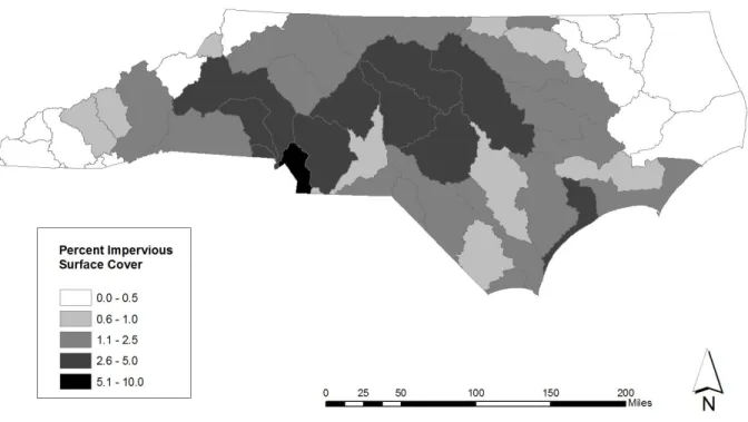
Population Growth and Impervious Surface Cover by Watershed
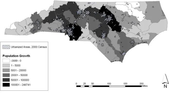
The majority of watersheds with high levels of growth, as indicated by population increase from 2000 to
2007 and percent impervious surface cover, are located in the central and western-central parts of the
state, as seen below in Figures 1 and 2. Three watersheds grew by over 100,000 (the Lower Catawba,
Upper Neuse and Rocky watersheds), another four by 50,000 to 100,000 (Upper Cape Fear, Upper
Catawba, Haw and Upper Yadkin), and seven more by 20,000 to 50,000 (Deep, Upper French Broad,
Lower Cape Fear, New, Lower Yadkin, Northeast Cape Fear, and South Yadkin). The watersheds with the
fastest-growing populations, not surprisingly, contain the majority of North Carolina’s major urbanized
areas, shown in Figure 1.
28
Figure 2. Percent impervious surface cover by watershed. Data obtained from National Land Cover Database (U.S. Department of Interior, no date).
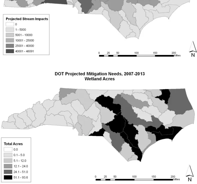
DOT Projected Mitigation Needs in Relation to Growth Indicators
According to the EEP’s procedures, mitigation credits are accumulated in response to projected needs of
the NC DOT. Thus the NC DOT’s predicted impacts are considered to be an important factor in this
analysis. NC DOT predicted impacts are discussed here first in relationship to growth indicators. The NC
DOT’s predictions for stream and wetland mitigation needs by 2013 are shown in Figure 3, below. As
seen in the figure, the spatial distribution of the NC DOT’s projected stream impacts differs notably from
that of the projected wetland impacts, with stream impacts more concentrated in the western half of
the state and wetland impacts more concentrated in the eastern part of the state.
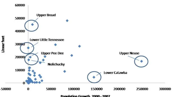
Scatter plots show the NC DOT’s predicted stream and wetland impacts plotted against the amount of
recent population growth by watershed (Figure 4). While these plots show a generally positive trend
29
there are a number of outlier watersheds with either high growth but low predicted mitigation needs, orlow growth but high predicted mitigation needs. The notable outliers are indicated in Figure 4.
30
31
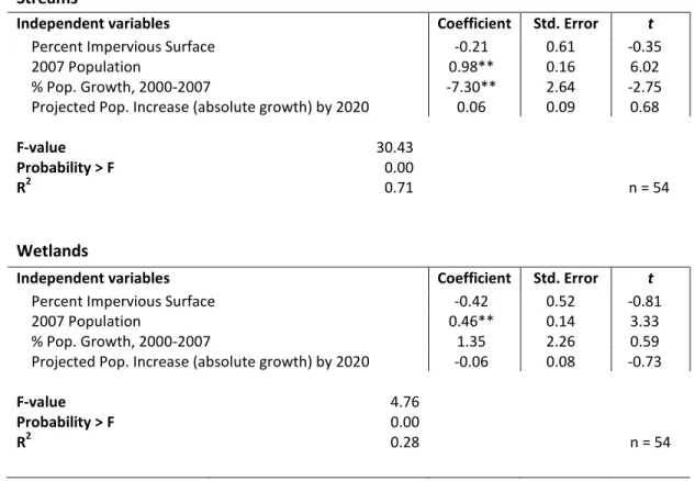
In order to determine more precisely whether the NC DOT’s predicted mitigation needs correspond withareas of high growth by watershed across the state, regression analysis was performed, with the NC
DOT’s projected mitigation needs for 2013 as the dependent variable and selected growth indicators as
the independent variables. The results of regression are given in Table 3, below. No variable exhibited a
VIF value above 3.04 in this model. As shown in the table, the model is significant (Probability > F = 0.00,
with an R2 value of 0.71 for predicted stream impacts and 0.28 for predicted wetland impacts.
Table 3. Results of regression analysis showing the influence of growth indicators on the NC DOT’s projected impacts by watershed.
Notes: Dependent variables are the NC DOT’s projected impacts to 2013 for streams and wetlands, respectively. All variables underwent logarithmic transformation prior to running regression.
Ψ
p < 0.10; * p<0.05; **p<0.01 Streams
Independent variables Coefficient Std. Error t
Percent Impervious Surface -0.21 0.61 -0.35
2007 Population 0.98** 0.16 6.02
% Pop. Growth, 2000-2007 -7.30** 2.64 -2.75
Projected Pop. Increase (absolute growth) by 2020 0.06 0.09 0.68
F-value 30.43
Probability > F 0.00
R2 0.71 n = 54
Wetlands
Independent variables Coefficient Std. Error t
Percent Impervious Surface -0.42 0.52 -0.81
2007 Population 0.46** 0.14 3.33
% Pop. Growth, 2000-2007 1.35 2.26 0.59
Projected Pop. Increase (absolute growth) by 2020 -0.06 0.08 -0.73
F-value 4.76
Probability > F 0.00
32
The NC DOT’s projected stream impacts exhibit a significant positive correlation with 2007 population(coefficient of 0.98), and a significant negative correlation with percent population growth from 2000 to
2007 (coefficient of -7.3). The magnitude of the coefficients cannot be used to directly describe the
strength of the correlation because the regression was run using logarithmically transformed data. Two
other growth indicators, including percent impervious surface cover and population growth projections
by 2020, show no significant correlation with the NC DOT’s projected stream impacts. Looking at the NC
DOT’s projected wetland impacts, only the 2007 watershed population shows a significant correlation
(coefficient 0.46) while the three other growth indicators show no significant relationship with projected
impacts.
EEP Mitigation Credits in Relation to Growth Indicators and DOT Projections
The mitigation credits acquired by the EEP exhibit a similar trend to the NC DOT’s projected impacts, in
that the majority of 8-digit watersheds with high levels of stream mitigation are located in the western
portion of the state, while the majority of acquired wetland credits are in the eastern portion of the
state (Figure 5, below). There are fourteen 8-digit HUC watersheds containing no wetland mitigation
credits at all, (including Upper Dan, Nolichucky, Roanoke Rapids, Middle Roanoke, Watauga,
Tuckasegee, Albemarle, Lower Catawba, Hiwassee, Tugaloo, Lynches, Ocoee, Nottoway and Blackwater
– the last two of which are under two square miles in area) and nine watersheds containing no stream
mitigation credits (Carolina Coastal-Sampit, Albemarle, Lower Catawba, Hiwassee, Tugaloo, Lynches,
Ocoee, Nottoway and Blackwater), shown in white on the maps below (Figure 5).
The scatter plots in Figure 6 show the EEP’s available stream and wetland mitigation credits plotted
against population growth by watershed. Similarly to those of the NC DOT predicted impacts, above,
these plots show a generally positive trend between the amount of accumulated mitigation and the
level of population growth by watershed. They also show that there are a number of outlier watersheds
that exhibit either high population growth but low accumulated mitigation, or low growth but high
33
34
35
The relationships between the EEP’s acquired credits, the NC DOT’s projected needs by 2013, and majorurbanized areas are mapped in Figure 7, below. Speckled watersheds in the figures indicate credit
deficits, calculated by subtracting the NC DOT’s forecasted impacts from the EEP’s acquired mitigation.
At least ten watersheds were predicted to have deficits for wetland mitigation, and at least fifteen for
stream mitigation if the EEP did not acquire additional mitigation in those watersheds.
As seen in Figure 7, below, the three largest urbanized areas in North Carolina – including the Triangle,
the Triad, and Charlotte regions – spatially correspond with credit deficits for stream mitigation in the
Lower Catwaba, Upper Yadkin, Haw and Upper Neuse watersheds. Similarly, the Lower Catawba and the
Haw, two watersheds containing major urban areas, have credit deficits for wetlands. Of these, the
Lower Catawba (containing Charlotte) has the largest mismatch between population growth and
acquired credits, given that it is one of the fastest-growing watersheds in the state, by population, but
by 2007 the EEP had acquired neither wetland nor stream mitigation credits there. The Albemarle
watershed, also lacking either type of mitigation credit, shows moderate levels of population growth
(growing by over 15,000 people between 2000 and 2007).
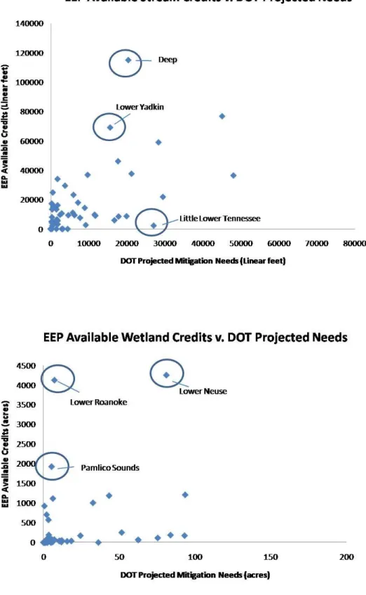
Scatter plots showing the NC DOT’s predicted impacts on the x-axis and the EEP’s available mitigation
credits for streams and wetlands on the y-axis are shown in Figure 8, below. Plots for both streams and
wetlands indicate a general positive trend; that is, as the NC DOT’s projected impacts increase, so do the
EEP’s available mitigation credits. More watersheds exhibit credit surpluses than credit deficits. In some