1236.pdf

(1)

ABSTRACT

CATHERINE CHERYL BODUROW. A Modified Method for Determination of

Free Styrene Glycol in Human Blood. (Under the Direction of STEPHEN M.

RAPPAPORT, Ph.D.)

Partitioning of free styrene glycol in plasma and packed red blood cells

was investigated in this study. Allyl benzene glycol was synthesized and used as

an internal standard in the procedure. It was determined there was no significant

difference in the styrene glycol concentrations in the plasma and red blood cells

layers (B=0.08, SE=1.01) of dosed blood samples. This result suggested that

free styrene glycol distributes uniformly throughout whole blood. The plasma

layer was chosen for analysis in this study and free styrene glycol concentrations

were determined in 85 plasma samples using the developed methodology of this

study. Samples and exposure data were obtained from three reinforced plastic

industry companies in the state of Washington. The exposure data investigated

were: eight-hour air styrene concentrations, whole blood styrene concentrations

and urinary metabolite (sum of mandelic and phenylglyoxylic acids)

concentrations. Companies #1,2 and 3 afforded the following number of plasma

samples, respectively: 31,17 and 17. Fourteen and six replicate measurements

and sets of exposure data were obtained for Companies # 1 and 2, respectively,

approximately one year after initial monitoring. Statistical analysis regressing

exposure data and plasma styrene glycol concentrations against exposure data

for single and replicate observations are presented in this work. Our findings

vary depending upon the company sampled. Company # 3 produced statistically

(2)

Ill

ACKNOWLEDGEMENTS

This work is dedicated to Mathukutty whose love and devotion have

unselfishly encouraged my graduate studies. I thank the Lord each day for

bringing him into my life.

I would like to acknowledge my advisor, Steve Rappaport, and my

readers. Dr. Lori Todd and Dr. Louise Ball, for their assistance in the preparation of this report. I am also indebted to Dr. Hans Kromhout for his statistical expertise and to Mary Ellen Tucker, MLS. for her assistance in locating technical

information.

Many thanks are due to my family and friends who have provided much support the past two years . In particular, I am eternally grateful to my parents whose endless encouragement and faith in my abilities have given me strength.

This project was conducted as part of a graduate training program and

was supported in part by a Centers For Disease Control Grant, grant number

(3)

TABLE OF CONTENTS

I. INTRODUCTION...1

1. Biological Monitoring...1

2. Styrene Exposure in the Reinforced Plastic Industry...5

3. The Metabolism of Styrene...6

4. Purpose of Study...8

II. METHODS AND MATERIALS...9

1. Plasma Samples and Exposure Data...9

2. Experimental...10

2.1. Materials and Instrumentation... 10

2.2. Synthesis of 3-Phenyl-1,2-propanediol (Allyl benzene glycol)...10

2.3. Styrene Glycol Partitioning in Human Plasma and Red Blood Cells...11

2.4. Analysis of Styrene Glycol in Workers' Plasma Samples...12

3. Statistical Analysis...13

3.1. Regression Analysis for Partitioning Experiment...13

3.2. Regression Analysis for Workers' Plasma Samples...13

III. RESULTS AND DISCUSSION...14

1. Synthesis of 3-Phenyl-1,2-propanediol (Allyl benzene glycol)...14

2. Styrene Glycol Partitioning in Human Plasma and Red Blood

Cells...16

2.1. Experimental Analysis...16

2.2. Statistical Analysis...17

3. Analaysis of Workers' Plasma Samples...25

3.1. Experimental Analysis...25

3.2. Statistical Analysis of Exposure Data...26

3.3. Statistical Analysis of Workers' Plasma Samples...43

3.4. Statistical Analysis of Replicate Exposure Data and Workers' Plasma Samples...56

4. General Discussion...67

IV. CONCLUSIONS...68

(4)

VII. BIBLIOGRAPHY...70

(5)

LIST OF FIGURES

FIGURE

1. Sites of uptake, target tissue, and media for monitoring of xenobiotic

compounds...2

2. Proposed Metabolic Pathways of Styrene...7

3. Proposed Mechanism for Allyl Benzene Glycol Formation...15

4. Whole Blood Styrene Glycol Concentration VS Serum Styrene Glycol

Concentration...18

5. Air Styrene Concentration VS Blood Styrene Concentration

(Company* 1)...34

6. Air Styrene Concentration VS Urinary Metabolite Concentration

(Company* 1)...35

7. Blood Styrene Concentration VS Urinary Metabolite Concentration

(Company* 1)...36

8. Air Styrene Concentration VS Blood Styrene Concentration

(Company #2)...37

9. Air Styrene Concentration VS Urinary Metabolite Concentration

(Company #2)...38

10. Blood Styrene Concentration VS Urinary Metabolite Concentration

(Company #2)...39

11. Air Styrene Concentration VS Blood Styrene Concentration

(Company #3)...40

12. Air Styrene Concentration VS Urinary Metabolite Concentration

(Company #3)...41

13. Blood Styrene Concentration VS Urinary Metabolite Concentration

(6)

VII

14. Air Styrene Concentration VS Average Plasma Styrene Glycol

Concentration (Company* 1)...47

15. Blood Styrene Concentration VS Average Plasma Styrene Glycol Concentration (Company* 1)...48

16. Urinary Metabolite Concentration VS Average Plasma Styrene Glycol Concentration (Company* 1)...49

17. Air Styrene Concentration VS Average Plasma Styrene Glycol Concentration (Company #2)...50

18. Blood Styrene Concentration VS Average Plasma Styrene Glycol

Concentration (Company #2)...51

19. Urinary Metabolite Concentration VS Average Plasma Styrene Glycol Concentration (Company #2)...52

20. Air Styrene Concentration VS Average Plasma Styrene Glycol Concentration (Company #3)...53

21. Blood Styrene Concentration VS Average Plasma Styrene Glycol

Concentration (Company # 3)...54

22. Urinary Metabolite Concentration VS Average Plasma Styrene Glycol Concentration (Company # 3)...55

A-1. NMR of 3-phenyl-1,2-propanediol (allyl benzene glycol)...75

A-2. Mass Spectrum of allyl benzene glycol derivative (ABG-PFB)...76

A-3. Gas Chromatogram of Typical Plasma Sample...77

(7)

UST OF TABLES

TABLE

1. Plasma and Red Blood Cells Partitioning Experiment Data...19

2. Model Definitions for Partitioning Experiment...22

3. Summary Statistics for Partitioning Experiment...22

4. Plasma, Red Blood Cells and Whole Blood Concentrations...23

5. Workers' Styrene Glycol Concentrations and Exposure Data...28

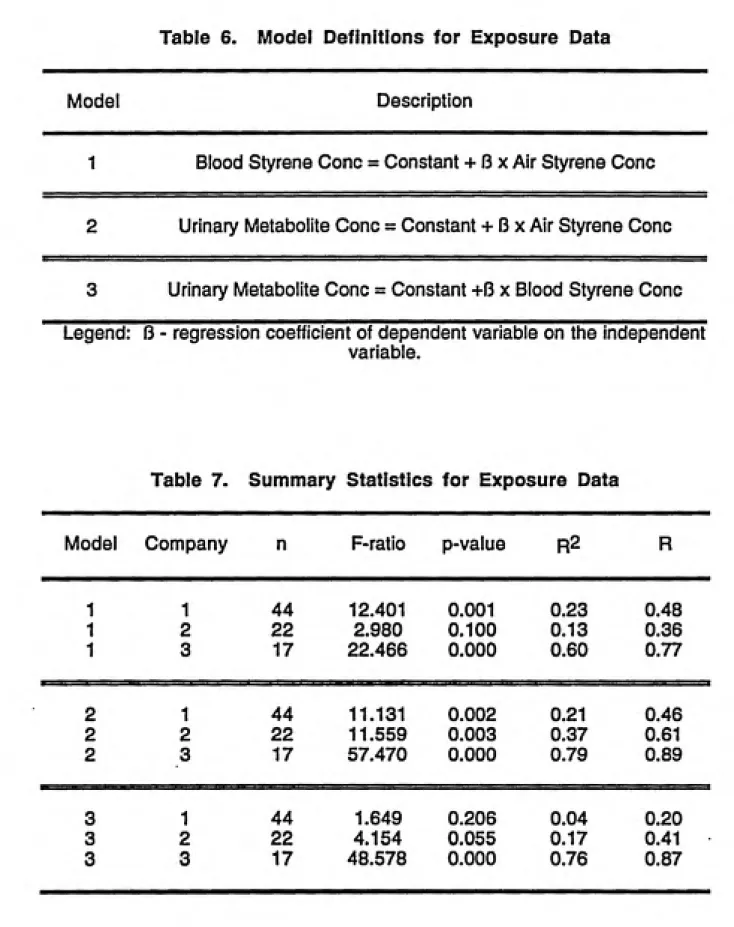
6. Model Definitions for Exposure Data...32

7. Summary Statistics for Exposure Data...32

8. Model Definitions for Workers' Plasma Samples...44

9. Summary Statistics for Workers' Plasma Samples...44

10. Replicate Worker's Styrene Glycol Concentrations and Exposure Data...57

11. Model Definitions for Exposure Data...58

12. Summary Statistics for Replicates' Exposure Data...58

13. Model Definitions for Workers' Plasma Samples...60

(8)

tx LIST OF ABBREVIATIONS

ABG

ABG-PFB

ANOVA

cone

BCD

GC

marker

MS

PFB

SG

SG-PFB

allyl benzene glycol

pentafluorobenzoyl ester of allyl benzene glycol

Analysis of Variance

concentration

electron capture detector

gas chromatograph

biological marker mass spectrometer

pentafluorobenzoyl chloride

styrene glycol

(9)

I. INTRODUCTION

1. Biological Monitoring

Occupational hygienists have traditionally monitored air concentrations to

evaluate human exposure to chemicals in the workplace. The growing necessity,

however, to quantify a worker's actual body burden has enabled hygienists to

make use of the emerging biological monitoring field (Fiserova-Bergerova, 1990).

A basic definition of biological monitoring is the measurement of an internal

exposure through the analysis of a biological specimen (Zielhuis, 1978). Wogan

(1989) defines biological monitoring as measurements made on cells, tissues, or

body fluids of exposed people with the intent to determine an internal or

biologically effective dose on an individual basis. Several media suitable for

biological monitoring are represented in Figure 1. The most common media are

exhaled air, blood and urine (Hulka, 1990 and Bernard, 1986).

There are several advantages to the use of biological monitoring as a

supplement to environmental monitoring. Biological monitoring can more

adequately determine susceptible groups of individuals than environmental

monitoring. Factors such as age, sex, body fat, intake of drugs and alcohol, and

socioeconomic status will affect an individual's uptake and metabolism of a

chemical (Guidotti, 1988). Secondly, it may be easier to estimate external

exposure by utilizing the individual as the sampling instrument. For example, if

(10)

ABSORPTION

Exfoli¬ ation

Skin

(Sweat)

INHALATION

Exhala¬ tion

Respiratory

Tract

Developing

Organs

~Pf^

\ ( Blood j ^

(^^

"7K

Kidney

( Urine j

INGESTION

\/

Gl-Tract

/salivaj

Liver

(Feces)

.KEY.

O

Target Tissues

Mediator

Biological

Monitoring

Figure 1. Sites of uptalce, target tissue, and media for monitoring of

(11)

practices and respiratory minute volume are not considered by environmental

monitoring. These factors contribute to a worker's body burden. It should also

be recognized that people are exposed to many chemicals simultaneously

through different pathways. Biological monitoring allows investigation of total

body burden which may aid in health risk assessment (Committee on Biological

Markers of the National Research Council, 1987). Finally, and perhaps most

importantly, biological monitoring offers the opportunity to consider individual

variability among those exposed (Hattis, 1987).

Although several advantages in favor of biological monitoring exist, the

method also possesses its disadvantages. People are the sampling instrument

in biological monitoring. This may be inconvenient for some individuals and

cause others unneeded anxiety. Although this field is rapidly developing, it is a

fact that many biological monitoring procedures for chemicals and/or their

metabolites do not yet exist. It is also important to consider that investigators are

not yet capable of producing reliable data on an individual monitoring basis.

Finally, biological monitoring may not be the appropriate method of evaluation

when external exposures vary greatly with time and the chemical of interest

exerts an acute effect on the individual (Zielhuis, 1978).

Griffith (1989) defines a biological marker as "any measurable

biochemical, physiological, cytological, morphological, or other biological

parameter obtainable from human tissues, fluids, or expired gases, that is

associated (directly or indirectly) with exposure to an environmental pollutant."

(12)

~ ." ͣ"•"--«V*f—^=. '

before a marker is chosen (Schulte, 1987). This will determine the validity of the

use of a marker at low exposure levels. Adducts of endogenous

macromolecules, such as DNA or proteins, may also indicate if damage and/or

repair have occurred due to chemical exposure (Perera, 1987). Another form of

markers of exposure or effect are cellular changes (Hulka, 1990). Cellular

changes may in fact be a link to carcinogenesis found in individuals exposed to

certain chemicals (Garner, 1985). Finally, the amount of time before a marker

appears and the persistance of the marker are important considerations. The

half-lives of chemicals may vary dramatically in different "compartments" of the

body. Many decisions in biological monitoring are indeed based upon biological

half-lives of chemicals and markers (Droz, 1989 and Monster, 1991). Regardless

of the choice of marker, Schulte (1987, 1989 and 1991) emphasizes the

importance of validation studies, including determinations of sensitivity,

specificity, and predictive value, before a marker is used in an epidemiologic

study.

Biological monitoring is not a new concept. Hints of biological monitoring

date back to the early 20th century when methods were developed more actively

in Europe than in the United States (Lowry, 1986). The past two decades have

yielded many advances worldwide. Of course, the appropriate use of biological

monitoring is as a complement to environmental monitoring and rigorous

epidemiologic designs (Brown, 1989). The field will continue to grow and may

act as the bridge between laboratory and epidemiologic assessment studies in

(13)

2. Styrene Exposure in the Reinforced Plastic industry

Chemical and Engineering News (1992) recently reported that styrene

monomer production has reached an all-time annual high of 9 billion lbs in the

United States . It also reported that combined quantities of polystyrene,

styrene-acrylonitrile and styrene-acrylonitrile-butadiene-styrene thermoplastic resins amounted to

approximately 7.3 billion lbs in 1991 production.

Although the reinforced plastic industry consumes less than ten percent of

the world's styrene production, the industry experiences the greatest exposures

to styrene. The primary raw material used in the reinforced plastic industry is

unsaturated polyester resin dissolved in styrene. The fabrication process adds

organic peroxides to the resins to initiate polymerization between the unsaturated

polyester resin and styrene. This produces the hard polymer which is essential

for many durable items, such as boats and automobiles (Tossavainen, 1978).

In the reinforced plastic industry, styrene primarily enters the body through

the respiratory system (MaIek, 1986). Dermal exposure may be avoided by strict

use of protective clothing and gloves. Brooks (1980) showed that skin protection

reduced the risk of dermatitis from styrene. In addition, Brooks also found that

"percutaneous absorption of styrene was not significant and indeed did not

significantly contribute to the body burden of styrene of workers engaged in hand

lay-up operations." Berode (1985) and Wieczorek (1985) reported similar results

in studies of percutaneous absorption of styrene. It is for this reason that styrene

exposure is normally assessed by measuring air concentrations.

Mortality studies performed by Okun (1985) and Wong (1990) of

styrene-exposed workers in the reinforced plastics industry did not yield a significant

(14)

3. The Metabolism of Styrene

The uptake of styrene vapor from the lungs has been investigated and Is

reported to be 63% of the inspired quantity (Engstrom, 1978). Ramsey (1978)

found approximately 97% of the absorbed styrene was cleared from the body by metabolism, and Teramoto (1979) showed styrene's biological half-life in the

human body to be 40 minutes in the rapid phase and 180 minutes in the slow

phase.

The metabolism of styrene has been extensively studied and is

summarized in Figure 2 (Lof, 1983). The first step of the proposed metabolic

pathway is the formation of styrene-7,8-oxide (phenyloxirane) from catalysis by microsomal cytochrome P-450 (Watabe, 1978). The epoxidation of styrene may

also be catalyzed by blood erythrocytes and lymphocytes (Norppa, 1983).

Styrene-7,8-oxide may then spontaneously hydrate to styrene glycol (1-phenyl-1,2-ethanediol) or be converted by microsomal epoxide hydratase (Dansette,

1978). Next, styrene glycol may either be conjugated with B-glucuronic acid

(Pantarotto, 1978) or oxidized to mandelic acid which can be further oxidized to

phenylglyoxylic acid (Bardodej, 1966). Mandelic acid may also oxidize to benzoic

acid which has been shown to conjugate with glycine (Leibman, 1975).

Another metabolic pathway primarily found in animals acts as a minor

pathway In humans. Styrene-7,8-oxide conjugates with glutathione in the

presence of glutathione S-transferase (Boyland, 1965). These conjugates will

generally degrade to mercapturic acids (James, 1967).

A minor amount of ring hydroxylation may occur at the 1,2- or 3,4-position of styrene and small quantities of phenyl ethanols and phenylacetaldehyde are also produced (Pantarotto, 1978). Several other metabolites have been identified

(15)

OH

I

CH-CH3 _CH=CH2

CH=CH2 CH=CH2

1-PHENYLETHANOL

CH2-CH2-OH

STYRENE

CH-CH2

OH

STYKENE-3,4-OXIDE 4-VINYLPHENOL

OH I

CH-CH2-SR

2-PHENYLETHANOL

CH2-CHO

PHENYLACETALDEHYDE

STYRENE-7,8-OXIDE

OH OH

I I CH-CH2

S-(2-PHENYL-2-HYDROXYETHYL)

GLUTATHIONE

SR

I

CH-CH2OH

CH2-COOH

PHENYLACETIC ACID

CH2CONHCH2COOH

STYRENE GLYCOL

OH

S-(l-PHENYL-2-HYDROXYETHYL)

GLUTATHIONE CONJUGATION WITH GLUCURONIC ACID

CH-COOH COOH

MANDELIC ACID BENZOIC ACID PHENACETURIC ACID

O

I

C-COOH

0

I

C-NHCH2COOH

PHENYLGLYOXYLIC ACID HIPPURIC ACID

(16)

8

2-phenylethanol, p-hydroxymandelic acid, p-hydroxybenzoic acid, and

p-hydroxyhippuric acid (Pantarotto, 1978).

Although approximately 85% of absorbed styrene is eliminated as

mandelic acid and 10% as phenylglyoxyiic acid in the urine (Guillemin, 1979), a small quantity of unchanged styrene may also be excreted in the urine (Dolara, 1984). In addition, Engstrom (1978) reported that the remainder of absorbed

styrene, approximately 2%, was exhaled unchanged.

4. Purpose of Study

It is clear that several media-exhaled air, blood and urine--may be used in

the biological monitoring of styrene-exposed workers. Lof has developed several methods for the assessment of styrene exposure in workers (1983, 1986). Of

particular interest is a method for determination of free styrene glycol in whole

blood which has been used in correlations with air styrene concentrations (Lof, 1986). It was our intention to streamline this procedure so that styrene glycol could be determined in human plasma or packed red blood cells rather than in whole blood.

The specific goals of this study were: a) to synthesize an appropriate internal standard for the procedure; b) to develop methodology for the determination of free styrene glycol in human plasma and packed red blood cells; c) to test the new method in a styrene-exposed population; and d) to compare plasma styrene glycol concentrations with styrene in air and blood and with

(17)

II. METHODS AND MATERIALS

1. Plasma Samples and Exposure Data

Plasma samples and exposure data were obtained from a group at the

University of Washington which conducted a study of styrene exposure in the

reinforced plastic industry. Blood samples and exposure data were collected at

three companies in the state of Washington over a two year period. Immediately

after collection, the blood samples were separated into plasma and red blood

cells layers and stored at -80 ^C prior to analysis. Exposure to styrene was

determined by personal monitoring over the eight-hour work shift. Styrene was

also measured in whole blood, and mandelic and phenylglyoxylic acid were

measured in the urine.

The number of workers monitored at Companies #1, #2 and #3,

respectively, were: 31,17 and 17. Replicate measurements and blood samples

were obtained from selected workers approximately one year after initial

monitoring at Companies #1 and #2. Company #1 yielded fourteen replicates

(18)

10

2. Experimental

2.1. Materials and Instrumentation

Reagents and chemicals. All chemicals were of reagent grade and used without further purification. Formic acid, hydrogen peroxide, allyl benzene, sodium hydroxide, hexanes, pentafluorobenzoyi chloride, methanol and styrene glycol were obtained from Aldrich Chemical Company, Inc. Ethyl acetate

was obtained from EM Science. Pyridine was obtained from Pierce.

Apparatus and conditions. Gas chromatography: A Varian model 3740 Gas

Chromatograph equipped with 63Ni electron-capture detector was

employed. A J & W Scientific DBS fused silica column (internal diameter =

0.25 mm, thickness = 0.25 nm, length = 30 meters) was used. The operating conditions were: column temperature, 240 OC; injector

temperature, 250 ^C; detector temperature, 320 ^C; carrier gas, He at a

flow rate of 1 mUmin; backflush, 0.5 minutes; length of run, 10 minutes.

Mass spectrometry: A Hewlett-Packard model 5890 Series II Gas

Chromatograph / 5971A Mass Selective Detector was employed under the

above operating conditions.

Nuclear Magnetic Resonance: Proton NMR spectra were obtained in deuterated

methanol on a Varian XL 400 MHz NMR fitted with Varian's 6.1 E Database.

2.2. Synthesis of 3-Phenyi-1,2-propanediol (Allyl benzene glycol)

Method adapted from Duverger-VanBogaert (1978)

Formic acid (96%) (30 mL, 0.80 mole) was placed in a 250 mL three-neck

round bottom flask equipped with a mechanical stirrer, thermometer and dropping

funnel. Hydrogen peroxide (30%) (7 mL, 0.2 mole) was then added dropwise at

room temperature. Dropwise addition of allyl benzene (98%) (6.7 mL, 51 mmole)

occurred thereafter. The reaction flask was next placed in an ice bath and the

(19)

exceed 35 ^C . The reaction was left stirring overnight at room temperature.

Excess reagent was removed by evaporation and addition of 7.5 mL saturated

sodium hydroxide hydrolysed the formyl esters of allyl benzene glycol. The

mixture was then extracted with 5 X 20 mL ethyl acetate. The combined organic

layers were dried over anhydrous sodium sulfate and were concentrated in vacuo

to approximately 15 mL. After cooling at 0 ^C, the clear oil (5.2g) was recovered

by filtration and distilled under vacuum. "Ih-NMR and Mass Spectrum

confirmation are found in Appendix A as Figure 1 and 2, respectively.

2.3. Styrene Glycol Partitioning in Human Plasma and Red Blood Cells

Derivatization method adapated from Duverger-Van Bogaert (1978)

Thirty mL of whole blood from a volunteer in our laboratory were drawn

into three ten mL heparinized vacutainers. The following procedure began within

one hour of the blood drawing. Twenty whole blood samples (ImL) were placed

in 4 mL capped glass vials. Ten piL of 1-Phenyl-1,2-ethanediol (styrene glycol)

solution in physiological saline (0.9% NaCI, by weight) were injected into each

whole blood sample, in duplicate, yielding the following levels: 100, 200, 300,

400, 500. 600, 700, 800, 900, 1000 ng styrene glycol/mL blood. The samples were gently inverted several times and then placed in a warm bath at 37 oc for 2

hours. The samples were next centrifuged at 2500 rpm for 8 minutes to separate

the plasma and red blood cells layers. Injection of 10 ^L of a solution of 100

ng/jiL 3-Phenyl-1,2-propanediol (allyl benzene glycol) in saline (0.9% NaCI, by

weight) afforded 1000 ng allyl benzene glycol as an internal standard in each

sample. The samples were extracted 3 times with ImL of ethyl acetate. If

emulsions occurred during the extractions, the samples were frozen in an

acetone/dry ice bath, warmed to room temperature and centrifuged at 1500 rpm

(20)

12

combined organic layers were dried over anhydrous sodium sulfate and

concentrated under nitrogen to a few drops. One mL of hexane was added to

each sample. Then 2 |xL pyridine and pentafluorobenzoyi chloride (1 p.L,

7 M-mole) were added to convert the glycols to the corresponding

pentafluorobenzoyi esters. The samples were mixed and placed in a heating

block at 50 ^c for 20 minutes. The samples were then dried under nitrogen flow.

In order to trap excess pentafluorobenzoyi chloride, 0.5 mL of an 85% solution of

methanol in water was added. Then the methanol/water layer was extracted with

one mL of hexane. Hexane standards containing 0, 30, 100, 300 and 1000 ng

styrene glycol/mL hexane and 1000 ng allyl benzene glycol/mL hexane in each

sample were derivatized as above. GC/MS confirmed the presence of the PFB

derivatives of styrene glycol and allyl benzene glycol. Two |j.I aliquots were then

injected into the GC/ECD (in triplicate). Three gas chromatograms were obtained

for each sample. A typical chromatogram is shown as Figure 3 in Appendix A.

The ratio of SG peak area and ABG peak area were compared to a standard

curve in order to determine the concentration of SG present in 1 mL hexane.

2.4. Analysis of Styrene Glycol In Workers' Plasma Samples

Each plasma sample (0.5mL) was gradually warmed to room temperature

and placed in a 4 mL capped glass vial. Injection of 10 ^L of a 100 ng/^iL

3-phenyl-1,2-propanediol (allyl benzene glycol) solution in physiological saline

(0.9% NaCI, by weight) afforded 1000 ng allyl benzene glycol as an internal

standard in each sample. The samples were gently inverted several times and

then placed in a warm bath at 37 OQ for 2 hours. The samples were extracted

with 3 times ImL of ethyl acetate and further processed as described in Section 2.3. GC/MS confirmed the presence of styrene glycol and allyl benzene glycol

(21)

(in duplicate). Ten samples were analyzed per experiment. A typical gas

chromatogram is shown as Figure 4 (Appendix A). The ratio of SG peak area

and ABG peak area were compared to a standard curve in order to determine the

concentration of SG present in 1 mL hexane.

3. Statistical Analysis

3.1. Regression Analysis for Partitioning Experiment

Statistical analysis of the partitioning experiment was conducted with SAS

software (SAS Institute, Gary, NC). Data were organized as shown in Table 1.

The variables considered in the regressions were: type (red blood cells or

plasma), initial styrene glycol concentration (100-1000 ng/mL), repeat (replicates

were run) and injection (1,2 or 3). These variables were regressed against the

final styrene concentration in different combinations as models.

3.2. Regression Analysis for Workers' Plasma Samples

The exposure data received from the University of Washington were

regressed against one another and also against the workers' plasma styrene

glycol concentrations via Lotus 123 software. Simple F-tests were also

(22)

III. RESULTS AND DISCUSSION

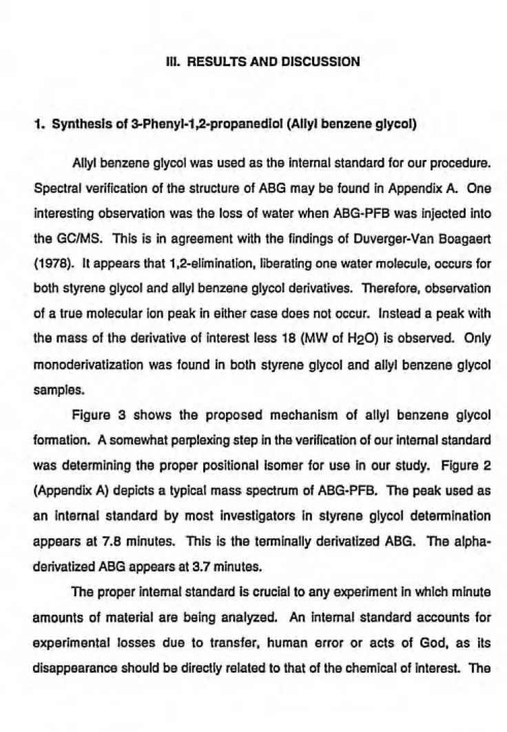
1. Synthesis of 3-Phenyl-1,2-propanediol (Allyl benzene glycol)

Allyl benzene glycol was used as the internal standard for our procedure.

Spectral verification of the structure of ABG may be found in Appendix A. One interesting observation was the loss of water when ABG-PFB was injected into the GO/MS. This is in agreement with the findings of Duverger-Van Boagaert

(1978). It appears that 1,2-elimination, liberating one water molecule, occurs for both styrene glycol and allyl benzene glycol derivatives. Therefore, observation

of a true molecular ion peak in either case does not occur. Instead a peak with

the mass of the derivative of interest less 18 (MW of H2O) is observed. Only

monoderivatization was found in both styrene glycol and allyl benzene glycol

samples.

Figure 3 shows the proposed mechanism of allyl benzene glycol

formation. A somewhat perplexing step in the verification of our internal standard

was determining the proper positional isomer for use In our study. Figure 2

(Appendix A) depicts a typical mass spectrum of ABG-PFB. The peak used as

an internal standard by most investigators in styrene glycol determination

appears at 7.8 minutes. This is the terminally derivatized ABG. The

alpha-derivatized ABG appears at 3.7 minutes.

The proper intemal standard is crucial to any experiment in which minute

amounts of material are being analyzed. An internal standard accounts for experimental losses due to transfer, human error or acts of God, as its

(23)

HO.

V=o + H2O2 H

FORMIC ACID

HYDROGEN

PEROXIDE

0

. 1

H-COOH PEROXYFORMIC ACID

r^

_^

^r^<

k^

0 H

AT.T.YT, BF:N7.KNE _/

0 1 0

= --H

^-^

+ OH

-o._'S

;c=o

H

"OH

O—C—H

X^

"-^^

ALLYL BENZENE GLYCOL

(24)

16

extraction and derivatization efficiencies of an internal standard will determine if it

is an appropriate comparison to the chemical being quantified. In addition, the gas chromatographic retention time of the internal standard in relation to the chemical sought is important. Normally, the ratio of the gas chromatographic peak areas of the chemical of interest to the internal standard are used to

determine concentrations of the chemical of interest. This was the method used in our study.

Allyl benzene glycol has proven to be the most appropriate internal standard to date for the analysis of styrene glycol concentrations. Three other possible internal standards were evaluated (DL-2-phenyl-1,2-propanediol,

4-methyl styrene glycol and 3-(4-hydroxyphenyl)-1-propanol); however, none of these compounds extracted and/or derivatized as well as allyl benzene glycol.

2. Styrene Glycol Partitioning in Human Plasma and Red Blood Cells

2.1. Experimental Analysis

It was our initial hypothesis that the concentrations of free styrene glycol in

the plasma and red blood cells layers of whole blood would be equal. Regardless, this experiment was crucial in proving that analysis of either plasma or red blood cells layers may be used to predict the amount of styrene glycol in

the other layer or whole blood.

The experiment consisted of twenty human whole blood samples which

(25)

we could recognize differences in duplicates, levels and between the plasma and

red blood cells layers.

It was observed during the separation of red blood cells and plasma that minimal breakage of red blood cells occurred. This is an important consideration

in subsequent statistical analysis, as red blood cell breakage will bias one's

results. The extractions were performed with great ease due to development of an unpublished freeze/centrifuge procedure in our laboratory (Jin, 1990). Typically, some samples of plasma and red blood cells emulse when extracted with ethyl acetate. This procedure yields optimal separation of the organic and

aqueous layers.

2.2. Statistical Analysis

Relevant data for the statistical analysis of the partitioning experiment may be found in Table 1. The variables investigated in the regression analyses were:

type (red blood cells or plasma), initial styrene glycol concentration (100-1000

ng/mL), replicate of type (1 or 2) and injection (1,2 or 3). Table 3 summarizes the

results of the regression analyses of variables against the final styrene glycol

concentrations obtained. Table 2 describes the various models presented in Table3. A two-way nested ANOVA model indicates a total of 5.7% error related to experimental procedure (2.0% due to the duplicate observations and 3.7% due

to the injections).

As shown in Table 3, the differences in the regresson coefficients for Models 1-3 and 4-6 are not significant. In fact, the regression coefficients of

Models 7 and 8 demonstrate that there is, essentially, no difference in the

regression coefficients for each injection. By grouping all of the data points together, we see that the difference in the regression coefficients for plasma and

(26)

18

lines is not significant (B = 0.08, SE = 1.01). This is a powerful and logical result,

as it suggests that styrene glycol distributes uniformly throughout whole blood.

Thus, the concentration of styrene glycol may be predicted in one layer (red

blood cells or plasma) by determination of the other.

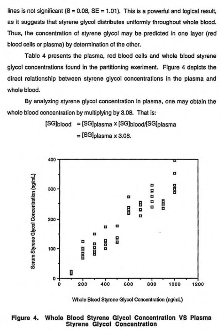
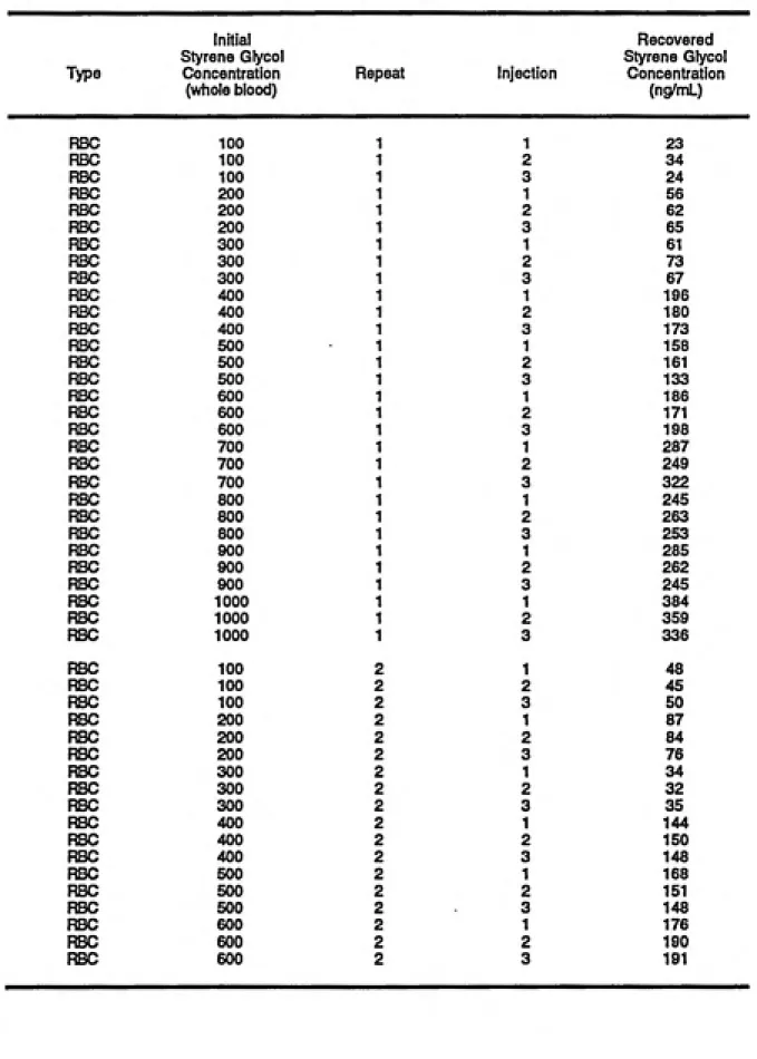
Table 4 presents the plasma, red blood cells and whole blood styrene

glycol concentrations found in the partitioning exeriment. Figure 4 depicts the

direct relationship between styrene glycol concentrations in the plasma and

whole blood.

By analyzing styrene glycol concentration in plasma, one may obtain the

whole blood concentration by multiplying by 3.08. That is:

[SG]biood = [SG]piasma x [SG]biood/[SG]piasma

= [SG]piasma X 3.08.

400

t

"S- 300

c

o

'H

a>

o

o 1 o

o c

£

CO

E

9

200-

100-1000 1200

Whole Blood Styrene Glycol Concentration (ng/mL)

Figure 4. Whole Blood Styrene Glycol Concentration VS Plasma

(27)

19

Table 1. Plasma and Red Blood Cells Partitioning Experiment Data

(28)

Table 1. (continued) 20 Initial Styrene Glycol Type Concentration (whole blood) Rep(

RBC 700 2

RBC 800 2

RBC 900 2

RBC 1000 2

PLASMA 100 PLASMA 100 PLASMA 100 PLASMA 200 PLASMA 200 PLASMA 200 PLASMA 300 PLASMA 300 PLASMA 300 PLASMA 400 PLASMA 400 PLASMA 400 PLASMA 500 PLASMA 500 PLASMA 500 PUSMA 600 PLASMA 600 PLASMA 600 PLASMA 700 PLASMA 700 PLASMA 700 PLASMA 800 PLASMA 800 PLASMA 800 PLASMA 900 PLASMA 900 PLASMA 900 PLASMA 1000 PLASMA 1000 PLASMA 1000

PLASMA 100 2

PLASMA 200 2

PLASMA 300 2

(29)

(30)

22

Table 2. Model Definitions for Partitioning Experiment

Model Description

1 Plasma SG Cone = B x Whole Blood SG Cone (injeetion=1, no intercept) 2 Plasma SG Cone = B x Whole Blood SG Cone (injection=2, no intercept) 3 Plasma SG Cone = B x Whole Blood SG Cone (injection=3, no intercept) 4 RBC SG Cone = B x Whole Blood SG Cone (injection=1, no intercept) 5 RBC SG Cone = B x Whole Blood SG Cone (injection=2, no intercept) 6 RBC SG Cone = B x Whole Blood SG Cone (injection=3, no intercept)

7 Plasma SG Cone = B x Whole Blood SG Cone (injection=1,2,3, no inter) 8 RBC SG Cone = B x Whole Blood SG Cone (injeetion=1,2,3, no intercept)

9 All Cone = B X Whole Blood SG Cone (injection=1,2,3, no intercept)

Legend: B - regression coefficient of styrene glycol concentration (ng/mL)

[dependent variable] on whole blood concentration (ng/mL).

Table 3. Summary Statistics for Partitioning Experiment

Model _Type n _Injection B SE R2

1 Plasma 20 1 0.331 0.0128 0.97

2 Plasma 20 2 0.332 0.0121 0.98

3 Plasma 20 3 0.311 0.0093 0.98

4 RBC 20 1 0.337 0.0134 0.97

5 RBC 20 2 0.322 0.0114 0.98

6 RBC 20 3 0.317 0.0148 0.96

7 Plasma 60 all 0.325 0.0066 0.98

8 RBC 60 all 0.326 0.0076 0.97

9 Both 120 all 0.325 0.0050 0.97

Legend: B-regression coefficient of styrene glycol concentration (ng/mL)

(31)

23

Table 4. Plasma, Red Blood Cells and Whole Blood Concentrations

Repeat Injection

RBC Plasma Whole Blood

Styrene Glycol Styrene Glycol Styrene Glycol

Concentration Concentration Concentration

(ng/nnL) (ng/mL) (ng/mL)

23 18 100

34 20 100

24 15 100

56 102 200

62 68 200

65 84 200

61 89 300

73 103 300

67 81 300

196 99 400

180 124 400

173 100 400

158 122 500

161 120 500

133 135 500

186 224 600

171 273 600

198 219 600

287 245 700

249 230 700

322 256 700

245 274 800

263 292 800

253 240 800

285 260 900

262 252 900

245 261 900

384 298 1000

359 353 1000

336 302 1000

48 22 100

45 17 100

50 22 100

87 94 200

84 124 200

76 74 200

34 149 300

32 91 300

35 116 300

144 127 400

150 113 400

148 174 400

168 136 500

151 177 500

148 122 500

176 238 600

190 232 600

191 220 600

(32)

24

Table 4. (continued)

Repeat Injection

2 1 2 2 2 3 2 1 2 2 2 3 2 1 2 2 2 3 2 1 2 2 2 3

RBC Plasma Whole Blood

Styrene Glycol Styrene Glycol Styrene Glycol

Concentration Concentration Concentration

(ng/mL) (ng/mL) (ng/mL)

225 211 700

235 254 700

219 232 700

205 314 800

198 296 800

191 257 800

285 245 900

258 258 900

225 235 900

401 397 1000

374 287 1000

(33)

3. Analaysis of Workers' Plasma Samples

3.1. Experimental Analysis

Two important findings may be concluded from the partitioning experiment. Firstly, there is essentially no difference in the partitioning of dosed human whole blood samples into plasma and red blood cells layers. Secondly,

there is minimal variability in injections at one concentration level. These

considerations afforded a more streamlined analysis of the workers' samples. There were two reasons that plasma was chosen as the layer of human whole blood for analysis in this study. The first reason was that the plasma layer yielded slightly lower standard errors than the red blood cells layer in the regression analysis of the partitioning experiment. The second reason was that emulsions occur less frequently during extractions in plasma than red blood cells because the plasma layer of whole blood contains less protein than the red blood

cells layer.

The analysis of the workers' plasma samples occurred more than one year after collection of the blood. For the purposes of this study, we have assumed the degradation of styrene glycol over time will not affect our analysis. If this were not the case, it would be crucial to investigate how styrene glycol degrades

overtime.

Ten plasma samples were analyzed per experiment and new hexane standards of styrene glycol and allyl benzene glycol were prepared for each experiment. As the samples had been frozen for a long time, it was critical to

warm the samples slowly from -80 ^C. They were warmed in the following manner: -20 ^c freezer, 0 ^C freezer, 4 ^C refrigerator, room temperature and

(34)

26

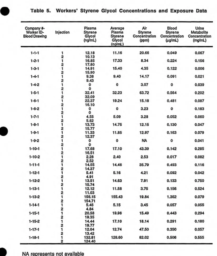
3.2. Statistical Analysis of Exposure Data

The exposure data received from the University of Washington are found

in Table 5. The data were evaluated by Company # and all pertinent regression

information may be found below the appropriate scatter diagram for each of the

described one-way Analysis of Variance (ANOVA) models (at the end of this section). Although the regression information in Table 7 of this section is summarized by model, the following results will be discussed by Company #.

Table 6 describes the regression models presented in Table 7. It is important to

note that the urinary metabolite concentration is the sum of mandelic acid and phenylglyoxylic acid concentrations. All replicate measurements for Companies

#1 and 2 are treated separately in the analyses to ensure the independence of

observations.

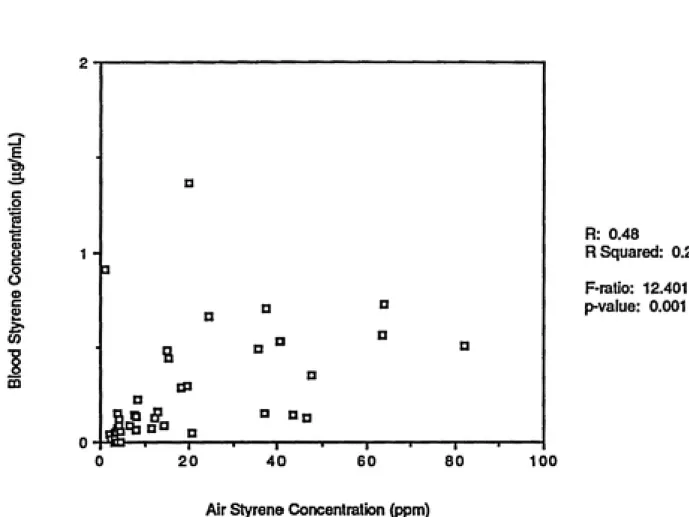
Company #1 exposure data (obtained from the University of Washington) are graphically represented in Figures 5-7. These are Models 1, 2 and 3,

respectively, in Table 6. Figure 5 plots air styrene concentration against blood

styrene concentration and yields a correlation coefficient of 0.48 (F-ratio =

12.401, p-value = 0.001, r2 = 0.23). Figure 6 depicts air styrene concentration

against urinary metabolite concentration. The correlation coefficient of 0.46

(F-ratio = 11.131, p-value = 0.002, r2 = 0.21) is similar to that in Model 1.

Finally, Figure 7 graphs blood styrene concentration against urinary metabolite concentration. These variables correlate poorly, yielding a R-value of 0.20

(F-ratio = 1.649, p-value = 0.206, r2 = 0.04). In summary, air styrene

concentration for Company #1 correlates acceptably with blood and urinary

metabolite concentrations. Each p-value is significant. Blood and urinary

(35)

Figures 8-10 graphically represent exposure data collected at Company #2. These are Models 1, 2 and 3, respectively, in Table 8. Figure 4 depicts the correlation of air styrene concentration and blood styrene concentration (R =

0.36, F-ratio = 2.980, p-value = 0.100, r2 = 0.13). A correlation coefficient of

0.61 (F-ratio = 11.559, p-value = 0.003, r2 = 0.37) is obtained when air styrene

and urinary metabolite concentrations are regressed (Figure 9). Regression of

blood styrene and urinary metabolite concentrations (Figure 10) yields a

correlation coefficient of 0.41 (F-ratio = 4.154, p-value = 0.055, r2 = 0.17).

Summarizing, Company #2 afforded p-values which are not significant when air styrene concentration is regressed against blood styrene concentration and when blood styrene and urinary metabolite concentrations are regressed. Regression of air styrene and urinary metabolite concentrations yielded a significant p-value.

Company #3 exposure data are graphically presented in Figures 11-13. These are Models 1, 2 and 3, respectively, in Table 6. Figure 11 shows air styrene concentration plotted against blood styrene concentration. These variables correlate well, yielding a R-value of 0.77 (F-ratio = 22.466, p-value =

0.000, r2 = 0.60). A correlation coefficient of 0.89 (F-ratio = 57.470, p-value =

0.000, r2 = 0.79) is found when air styrene and urinary metabolite concentrations are regressed (Figure 12). Figure 13 depicts the relationship

between blood styrene and urinary metabolite concentrations. The variables have a strong correlation coefficient of 0.87 (F-ratio = 48.578, p-value = 0.000,

r2 = 0.76). In summary. Company #3's exposure data correlates well with each

other.

(36)

28

Table 5. Workers' Styrene Glycol Concentrations and Exposure Data

Company #- Plasnia Average Air Blood Urine

Worker ID- Injection Styrene Plasnia Styrene styrene Metabolite

Blood Drawing Glycol Styrene Concentration Concentration Concentration

(ng/mL) Glycol

(nq/mL)

(ppm) (ag/rrL) (mg/mL)

1-1-1 1

2

12.18 10.13

11.16 20.66 0.049 0.067

1-2-1 1

2

16.85

17.80

17.33 8.34 0.224 0.156

1-3-1 1

2

14.91 15.90

15.40 4.35 0.122 0.006

1-4-1 1

2

9.38 9.43

9.40 14.17 0.091 0.021

1-4-2 1

2

0 0

0 3.07 0 0.039

1-5-1 1

2

32.41 32.09

32.23 63.72 0.564 0.202

1-6-1 1

2

22.37 16.10

19.24 15.18 0.481 0.087

1-6-2 1

2

0

0 3.23 0 0.183

1-7-1 1

2

4.55

5.62

5.09 3.28 0.052 0.060

1-8-1 1

2

13.73

15.77

14.75 12.15 0.130 0.047

1-9-1 1

2

11.33 12.37

11.85 12.97 0.163 0.079

1-9-2 1

2

0 0

0 NA 0 0.041

1-10-1 1

2

17.68 16.51

17.10 43.39 0.142 0.285

1-10-2 1

2

2.28 2.52

2.40 2.53 0.017 0.082

1-11-1 1

2

14.55 14.37

14.46 35.79 0.493 0.116

1-12-1 1

2

5.41 4.91

5.16 4.21 0.092 0.042

1-12-2 1

2

13.51 15.74

14.63 7.91 0.133 0.750

1-13-1 1

2

12.12 11.03

11.58 3.75 0.156 0.524

1-13-2 1

2

156.15 154.71

155.43 19.84 1.362 0.079

1-14-1 1

2

5.46 4.84

5.15 3.45 0.057 0.055

1-15-1 1

2

20.58 19.35

19.96 15.49 0.443 0.294

1-15-2 1

2

14.44

19.77

17.10 18.14 0.291 0.180

1-17-1 1

2

12.04

13.42

12.74 47.50 0.350 0.057

1-18-1 1

2

132.81

124.40

128.60 82.02 0.506 0.555

(37)

Company #- Plasnna Average Air Blood Urine

Worker ID- Injection Styrene Plasnna Styrene Styrene Metabolite

Blood Drawing Glycol Styrene Concentration Concentration Concentration

(ng/mL) Glycol

(no/ml)

(ppm) (jig/mL) (mg/mL)

1-18-2 1

2

1.60 1.19

1.40 3.26 0.030 0.241

1-19-1 1

2

5.31

4.46

4.88 8.10 0.064 0.039

1-19-2 1

2

0 0

0 4.67 0 0.020

1-20-1 1

2

3.78

3.34

3.56 3.72 0.072 0.008

1-20-2 1

2

8.76 8.64

8.70 46.53 0.130 0.350

1-21-1 1

2

7.33 7.45

7.39 4.32 0.088 0.024

1-21-2 1

2

23.87

17.45

20.66 37.06 0.155 1.272

1-22-1 1

2

61.48 69.93

65.71 63.97 0.719 0.975

1-23-1 1

2

6.83 10.89

8.86 1.97 0.043 0.024

1-23-2 1

2

0.69 0.62

0.66 3.89 0 0.166

1-24-1 1

2

46.09 51.20

48.64 37.51 0.699 0.110

1-24-2 1

2

P2.79

29.56

26.17 24.60 0.660 0.125

1-25-1 1

2

132.04

145.44

138.74 1.12 0.904 0.318

1-26-1 1

2

7.31 9.80

8.56 4.51 0.058 0.044

1-26-2 1

2

3.92 4.61

4.26 3.56 0 0.051

1-27-1 1

2

30.27 22.23

26.25 19.56 0.299 0.192

1-28-1 1

2

7.78 15.21

11.50 6.65 0.091 0.159

2-32-1 1

2

105.61 110.40

108.01 51.87 0.135 1.749

2-33-1 1

2

121.19

134.15

127.67 70.83 0.015 2.287

2-34-1 1

2

193.66 196.52

195.09 64.21 0.124 0.324

2-34-2 1

2

16.20 22.97

19.58 85.15 0.017 0.192

2-35-1 1

2

107.18 120.14

113.66 51.38 0.325 0.886

2-36-1 1

2

144.52

134.72

139.62 12.48 0.120 0.299

2-37-1 1

2

7.70 8.48

8.09 18.77 0.132 0.084

(38)

Table 5. (continued) 30 Connpany #-Worker ID-Blood Drawing Injection Plasnna Styrene Glycol (ng/mL) Average Plasnia Styrene Glycol (ng/mL) Air Styrene Concentration (ppm) Blood Styrene Concentration (ng/mL) Urine Metabolite Concentration (mg/mL) 2-37-2 1 2 74.32 76.91

75.62 10.61 NA 0.133

2-38-1 1

2

26.19 27.16

26.68 9.85 0.176 0.326

2-38-2 1

2

485.41 478.59

482.00 6.98 0.150 0.109

2-39-1 1

2

31.32 38.97

35.15 19.29 0.410 0.580

2-40-1 1

2

4.38 5.41

4.90 0.55 0.001 0.005

2-41-1 1

2

5.55

6.11

5.83 2.57 0.016 0.066

2-42-1 1

2

31.98 23.54

27.76 0.96 0.020 0.002

2-43-1 1

2

12.17

9.22

10.70 1.86 0.031 0.004

2-44-1 1

2

3.37 3.89

3.63 0.49 0.009 0.005

2-44-2 1

2

27.75

26.73

27.24 1.12 0.001 0.005

2-47-1 1

2

14.32

13.26

13.79 13.90 0.047 0.319

2-48-1 1

2

14.76 14.39

14.58 56.83 0.125 0.212

2-48-2 1

2

437.35

440.88

439.11 61.31 0.052 0.251

2-49-1 1

2

37.24

37.09

37.17 43.53 0.054 0.419

2-49-2 1

2

150.86 163.64

157.25 76.38 0.747 1.456

3-52-1 1

2

6.43

13.40

9.91 3.33 0.027 0.399

3-53-1 1

2

30.09 26.88

28.48 22.46 0.153 0.572

3-54-1 1

2

4.91

4.43

4.67 4.21 0.054 0.083

3-55-1 1

2

100,70 106.20

103.45 42.95 0.504 1.779

3-56-1 1

2

0 0

0 1.36 0 0.046

3-57-1 1

2

5.81 7.27

6.54 1.78 0.020 0.059

3-58-1 1

2

17.22

20.62

18.92 160.90 0.351 2.645

3-59-1 1

2

171.21

163.28

167.25 134.90 0.582 2.001

3-60-1 1

2

0 0

0 4.40 0.003 0.021

(39)

31

Company #-Worker ID-Blood Drawing Injection Plasma Styrene Glycol (ng/mL) Average Plasma Styrene Glycol (ng/mL) Air Styrene Concentration (ppm) Blood Styrene Concentration (ng/mL) Urine Metabolite Concentration (mg^mL) 3-61-1 1 2 2.00 1.54

1.77 2.95 0.008 0.029

3-62-1 1

2

16.43 14.94

15.68 53.24 0.022 0.359

3-63-1 1

2

72.28 76.10

74.19 37.55 0.196 0.105

3-64-1 1

2

12.03 13.48

12.75 2.31 0.010 0.008

3-65-1 1

2

15.16 14.44

14.80 4.87 0.056 0.414

3-66-1 1

2

21.10 19.15

20.12 25.63 0.165 0.939

3-67-1 1

2

37.82

43.56

40.69 29.22 0.123 0.524

3-68-1 1

2

0 0

0 1.06 0.021 0.009

1-99-2 1

2

3.22

2.59

2.90 3.24 0 0.116

1-100-2 1

2

26.41 29.70

28.06 11.60 0.076 0.235

1-101-2 1

2

20.69

21.43

21.06 7.76 0.148 0.436

1-102-2 1

2

74.86

88.26

81.56 40.47 0.530 0.472

2-121-2 1

2

0 0

0 0.78 0.001 0.007

(40)

32

Table 6. Model Definitions for Exposure Data

Model Description

Blood Styrene Cone = Constant + B x Air Styrene Cone

Urinary Metabolite Cone = Constant + B x Air Styrene Cone

3 Urinary Metabolite Cone = Constant +B x Blood Styrene Cone

Legend: B - regression coefficient of dependent variable on the independent

variable.

Table 7. Summary Statistics for Exposure Data

Model _Company n F-ratio p-value R2 R

1 1 44 12.401 0.001 0.23 0.48

1 2 22 2.980 0.100 0.13 0.36

1 3 17 22.466 0.000 0.60 0.77

2 1 44 11.131 0.002 0.21 0.46

2 2 22 11.559 0.003 0.37 0.61

2 3 17 57.470 0.000 0.79 0.89

3 1 44 1.649 0.206 0.04 0.20

3 2 22 4.154 0.055 0.17 0.41

(41)

regression models. Company #1 correlates acceptably when air styrene

concentration is regressed against blood styrene and urinary metabolite

concentrations; however, blood styrene and urinary metabolite concentrations do

not correlate well. Company #2's exposure data produce p-values which are not

significant in two instances. However, a significant p-value is obtained when air

(42)

34

E

ͣ

&> 3>

c

.2

•E

U c

o

c

£

0}

CQ

R: 0.48

R Squared: 0.23

F-ratio: 12.401

p-value: 0.001

100

Air Styrene Concentration (ppm)

Figure 5. Air Styrene Concentration VS Blood Styrene Concentration

(43)

1

E,

c

.2

S "E

o

O

o (0 4)

R: 0.46

R Squared: 0.21

F-ratio: 11.131

p-vaiue: 0.002

100

Figure 6. Air Styrene Concentration VS Urinary l\/letabolite Concentration

(44)

36

t

E,

c

o

•E

(D U c

o

»

(0

ͣ

s

•c

R: 0.20

R Squared: 0.04

F-ratio: 1.649

p-value: 0.206

Blood Styrene Concentration (^g/mL)

(45)

E

s

ͣ

s

o

o c

o

O

o c o

t

CO

0.6-*-.

R: 0.36

R Squared: 0.13

F-ratio: 2.980

p-value: 0.100

100

Air Styrene Concentratbn (ppm)

Figure 8. Air Styrene Concentration VS Blood Styrene Concentration

(46)

38

t

E

S

5

(0

R: 0.61

R Squared: 0.37

F-ratio: 11.559

p-value: 0.003

100

Figure 9. Air Styrene Concentration VS Urinary iUletabolite Concentration

(47)

#

E

E,

c

.S

"E

o

CO

"S

R: 0.41

R Squared: 0.17

F-ratio: 4.154

p-value: 0.055

0.8

Blood Styrene Concentration (ng/rrL)

Figure 10. Blood Styrene Concentration VS Urinary lUletabolite

(48)

40

i

c

o

1

o

I

o c

S

CQ

R: 0.77

R Squared: 0.60

F-ratio: 22.466

p-value: 0.000

100 200

(49)

41

E

ͣ

&)

E,

c

.2

•E

O c

o

CO

•5

R: 0.89

R Squared: 0.79

F-ratio: 57.470

p-value: 0.000

200

(50)

42

C

o

I

"S

a> o

o

(0

•c

3

— " u

0 yp ͣ---1

R: 0.87

R Squared: 0.76

F-ratb: 48.578

p-value: 0.000

0.6

Blood Styrene Concentration Oig/mL)

Figure 13. Blood Styrene Concentration VS Urinary Metabolite

(51)

43

3.3. Statistical Analysis of Workers'Plasma Samples

Experimentally determined plasma styrene glycol concentrations from

workers in the reinforced plastic industry may be found in Table 5. The data

were evaluated by Company # and all pertinent regression information may be

found below the appropriate scatter diagram for each of the described one-way

ANOVA models (at the end of this section). Although regression information in

Table 9 is summarized by model, the following results will be discussed by

Company #. Table 8 describes the regression models presented in Table 9. All

replicate measurements for Companies #1 and 2 are treated separately in the analysis to ensure the independence of observations. The plasma styrene glycol

concentrations are represented as the average concentration of the two

injections.

Company #1 data are depicted in Figures 14-16. These are Models 1, 2

and 3, respectively, in Table 8. Figure 14 plots air styrene concentration against

average plasma styrene glycol concentration. The correlation coefficient is 0.48

(F-ratio = 9.815, p-value = 0.003, r2 = 0.23). Blood styrene concentration is

correlated with average plasma styrene glycol concentration in Figure 15. Here a

relatively good correlation coefficient of 0.60 (F-ratio = 101.790, p-value = 0.000,

r2 = 0.60) is observed. Figure 16 depicts the correlation of urinary metabolite

concentration and average plasma styrene glycol concentration. The correlation

is weak, yielding a R-value of 0.28 (F-ratio = 3.691, p-value = 0.062, r2 = 0.08).

Summarizing, Company #1 air and blood styrene concentrations appear to regress relatively well against the average plasma styrene glycol concentration.

However, urinary metabolite concentration does not regress as well against

(52)

44

Table 8. Model Definitions for Workers' Plasma Samples

IVIodei Description

Plasma SG Cone = Constant + B x Air Styrene Cone

Plasma SG Cone = Constant + B x Blood Styrene Cone

3 Plasma SG Cone = Constant + B x Urinary Metabolite Cone

Legend: B - regression coefficient of dependent variable on the independent

variable.

Table 9. Summary Statistics for Workers' Plasma Samples

Model Company n F-ratio p-value R2 R

1 1 44 9.815 0.003 0.23 0.48

1 2 22 1.740 0.202 0.08 0.28

1 3 17 7.878 0.013 0.34 0.58

2 1 44 101.790 0.000 0.60 0.77

2 2 22 0.654 0.428 0.03 0.17

2 3 17 56.913 0.000 0.79 0.89

3 1 44 3.691 0.062 0.08 0.28

3 2 22 0.476 0.498 0.02 0.14

(53)

45

Company # 2 data are presented in Figures 17, 18 and 19. These figures

are Models 1,2 and 3, respectively, in Table 8. Figure 17 shows air styrene

concentration plotted against average plasma styrene glycol concentration. A weak correlation coefficient of 0.28 is obtained (F-ratio = 1.740, p-value = 0.202,

r2 = 0.08). Figure 18 presents the correlation of blood styrene concentration

with average plasma styrene glycol concentration. A R-value of 0.17 (F-ratio =

0.654, p-value = 0.428, r2 = 0.03) demonstrates a very weak correlation. The

regression of urinary metabolite concentration and average plasma styrene glycol

concentration is shown in Figure 19. Another weak correlation coefficent, R =

0.14 (F-ratio = 0.476, p-value = 0.498, r2 = 0.02), is observed. In summary.

Company #2's exposure data do not correlate well with average plasma styrene

glycol concentration.

Figures 20-22 represent Models 1, 2 and 3, respectively, in Table 8.

These models investigate Plant #3's relationship to average plasma styrene

glycol concentration. Figure 20 depicts the regression of air styrene

concentration against average plasma styrene glycol concentration. A marginal

correlation coefficient of 0.58 (F-ratio = 7.878, p-value = 0.013, r2 = 0.34) was

found. Blood styrene concentration and average plasma styrene glycol

concentration are plotted in Figure 21. An exceptional R-value of 0.89 Is

obtained (F-ratio = 56.913, p-value = 0.000, r2 = 0.79). Figure 22 plots urinary

metabolite concentration against average plasma styrene glycol concentration,

yielding a marginal coefficient of 0.60 (F-ratio = 8.351, p-value = 0.011, r2 =

0.36). Company #3's exposure data regresses relatively well with the average

plasma styrene glycol concentraiton. Each p-value is significant.

Company #3 provides the best overall correlations for air styrene, blood

(54)

46

styrene concentrations correlate well with average plasma styrene glycol

concentration, yielding significant p-values. However, the correlation of urinary

metabolite concentration with average plasma styrene glycol concentration for

Company #1 yields only a marginally significant p-value. Company #2 does not

correlate well with average plasma styrene glycol concentration, affording non¬

(55)

47

E

ͣ

&)

s

CO

c

o

$0

o

O

I

a

o

c

S

O) s

cyj\j

-a

a 1

100-a

a

ͣ a

0-n o0-n

---J

D

R: 0.48

R Squared: 0.23

F-ratio: 9.815

p-value: 0.003

20 40 60 80 100

Figure 14. Air Styrene Concentration VS Average Plasma Styrene Glycol

(56)

48

200

t

CO

c

.2

I

c

» o

O

I

o>

&

e

100-R: 0.77

R Squared: 0.60

F-ratio: 101.790

p-value: 0.000

Blood Styrene Concentration Oxg/mL)

Figure 15. Blood Styrene Concentration VS Average Plasma Styrene Glycol

(57)

200

E

E S

c

o

ͣ

•?s

B 8

I

o

9

C £

e

S

100-R: 0.28

R Squared: 0.08

F-ratio: 3.691

p-value: 0.062

Urinary Metabolite Concentration (mg/mL)

Figure 16. Urinary IMetabolite Concentration VS Average Plasma Styrene Glycoi

(58)

.jm

50

1

E

S

§

ͣ

s

1

a

o

c £

o

S

500

400

300

200

100

B

3 D

0-^ .""i

20

—T"

40

—r—

60

—r—

80

R: 0.28

R Squared: 0.08

F-ratto: 1.740

p-value: 0.202

100

Figure 17. Air Styrene Concentration VS Average Plasma Styrene Glycol

(59)

t

¥

o

(0

1

"S

i

o

O

8

(3

a> c

2

a> o>

S

e

3UU

-ͤ

ͣ

a

400-

300-200- a

100-a

ͤ

a a

D

1

0^

k

,iA-ͤ

—1---' ͣ -I--->---1

R: 0.17

R Squared: 0.03

F-ratio: 0.654

p-value: 0.428

0.0 0.2 0.4 0.6 0.8

Figure 18. Blood Styrene Concentration VS Average Plasma Styrene Glycol

(60)

'-"^T?^^^^^^^^^-52

E

S

CO

c

o

$0

0)

5

1

9

C

o

t

o>

S

o

ouu

-D

•

D

400-

300-200- D

100-D

D

o\

1 n° °

Us ,

R: 0.14

R Squared: 0.02

F-ratio: 0.476

p-value: 0.498

Urinary Metabolite Concentrat'ion (mg/mL)

Figure 19. Urinary Metabolite Concentration VS Average Plasma Styrene Glycol

(61)

53

200

c

0)

CO

,c

c

.S

o

O

1

a

o c

£

o

S

o

100-R: 0.58

R Squared: 0.34

F-ratio: 7.878

p-value: 0.013

200

Figure 20. Air Styrene Concentration VS Average Plasma Styrene Glycol

(62)

54

200

E

»

CO

,c

c

o

"S

H

o

8

a

o i

s>

G

I

100

0-<Po-?-0.0

R: 0.89

R Squared: 0.79

F-ratio: 56.913

p-value: 0.000

—T---1---1---1---1---1---1---1---1---1---0.1 0.2 0.3 0.4 0.5 0.6

Figure 21. Blood Styrene Concentration VS Average Plasma Styrene Glycol

(63)

55

E

o

ͣE

o

O

o o

» c

£

o>

2

(0

uu

-D

00-D

D

ͣ

D

1

OH

I ^

D

---1---—,---,---D 1

R: 0.60

R Squared: 0.36

F-ratio: 8.351

p-value: 0.011

Urinary Metabolite Concentratbn (mg/mL)

Figure 22. Urinary Metaboiite Concentration VS Average Plasma Styrene Giycol

(64)

56

3.4. Statistical Analysis of Replicate Exposure Data and Workers' Plasma

Samples

Approximately one year after initial collection, replicate measurements for

air and blood styrene and urinary metabolite concentrations were collected for

Companies # 1 and # 2. Blood samples were also obtained at this time. Thirteen

sets of data came from Company #1 and five sets from Company #2. There

were no replicates measured for Company #3. For the purposes of our analysis,

the data from Companies #1 and 2 have been combined and the replicate

measurements have been averaged. The data are found in Table 10. All

pertinent regression information may be found below the appropriate scatter

diagram for each of the described one-way ANOVA models (at end of this

section).

Exposure data for replicate observations in Companies #1 and 2 are

graphically represented in Figures 23-25. These figures correspond to Models 1,

2 and 3, respectively, in Table 11. Figure 23 plots average air styrene

concentration against average blood styrene concentration. A weak correlation

coefficient of 0.14 (F-ratio = 0.347, p-value = 0.564, r2 = 0.21) is obtained.

Figure 24 depicts average air styrene concentration against average urinary

metabolite concentration. These variables correlate relatively well, yielding a

R-value of 0.50 (F-ratio = 5.271, p-value = 0.036, r2 = 0.25). The regression of

average blood styrene concentration against urinary metabolite concentration is

represented in Figure 25. A weak correlation coefficient of 0.30 (F-ratio = 1.511,

p-value = 0.237, r2 = 0.09) is obtained. In summary, when the averaged

exposure concentrations are regressed against one another, the only model

which yields a significant p-value is average air styrene concentration against

(65)

Table 10. Replicate Workers' Styrene Glycol Concentrations

and Exposure Data

57

Company

#-Worker

ID-Average

Plasma

Styrene Glycol (ng/mL)

Average

Air

Styrene

Concentration

(ppm)

Average

Blood

Styrene

Concentration

(tig/mL)

Average

Urine

Metabolite Concentration

(mg/mL)

1-4 4.70 8.62 0.046 0.030

1-6 9.62 9.20 0.241

0.135

1-10 9.75 22.96 0.079 0.184

1-12 9.89 6.06 0.113 0.396

1-13 83.50 11.80 0.759 0.302

1-15 18.53 16.82 0.367 0.237

1-18 65.00 42.64 0.268

0.398

1-19 2.44 6.38 0.032 0.029

1-20 6.13 25.12 0.101 0.179

1-21 14.02 20.69 0.122 0.648

1-23 4.76 2.93 0.021 0.095

1-24 37.41 31.06 0.679

0.117

1-26 6.41 4.04 0.029 0.048

2-34 107.34 74.68 0.070 0.258

2-38 254.34 8.42 0.163

0.217

2-44 15.43 0.80 0.005

0.005

2-48 226.84 59.07 0.089

0.232

(66)

58

Table 11. Model Definitions for Exposure Data

Model Description

Blood Styrene Cone = Constant + (3 x Air Styrene Cone

Urinary Metabolite Cone = Constant + B x Air Styrene Cone

3 Urinary Metabolite Cone = Constant +3 x Blood Styrene Cone

Legend: B - regression coefficient of dependent variable on the independent

variable.

Table 12. Summary Statistics for Replicates' Exposure Data

Model Company n F-ratio p-value R2 R

1 2 3

1+2 1+2 1+2

18 18 18

0.347

5.271 1.511

0.564

0.036

0.237

0.02

0.25 0.09

(67)

59