Inventory of complementary products with stock-dependent demand under vendor-managed inventory with consignment policy

Sharif University of Technology

Transactions E: Industrial Engineering http://scientiairanica.sharif.edu

Inventory of complementary products with

stock-dependent demand under vendor-managed

inventory with consignment policy

M. Hemmati, S.M.T. Fatemi Ghomi

_{, and M.S. Sajadieh}

Department of Industrial Engineering, Amirkabir University of Technology, 424 Hafez Avenue, Tehran, P.O. Box 1591634311, Iran. Received 23 September 2016; received in revised form 11 March 2017; accepted 6 May 2017

KEYWORDS Supply chain coordination; Inventory control; Complementary products; Stock-dependent demand; Consignment; Vendor-managed inventory.

Abstract. This paper proposes an integrated two-stage model, which consists of one vendor and one buyer for two complementary products. The vendor produces two types of products and delivers them to the buyer in distinct batches. Buyer stocks items in the warehouse and on the shelf. The demand for each product is sensitive to stock levels of both products. A vendor-managed inventory with consignment stock policy is considered. The number of shipments and replenishment lot sizes are jointly determined as decision variables in such a way that total prot is maximized. The numerical study shows that as complementation rate increases, the quantity of transfers and demand of both products increase. Hence, ignoring the complementation between products leads to the loss of some customers.

© 2018 Sharif University of Technology. All rights reserved.

1. Introduction

In the today's competitive market, individual opti-mization is not protable; hence, sharing information between supply chain members has become essential. Coordination can decrease supply chain costs and increase sales volume [1]. Supply chain coordination makes management more ecient to encounter real life uncertainty [2]. Literature review of the joint optimization of the vendor and buyer costs was rst started by Goyal [3]. He assumed that the vendor had innite production rate in presence of lot-for-lot policy. Banerjee [4] developed the model by assuming a nite rate. Goyal [5] generalized the model by relaxing

lot-*. Corresponding author. Tel.: +98 21 64545381; Fax: +98 21 66954569

E-mail addresses: m [email protected] (M. Hemmati); [email protected] (S.M.T. Fatemi Ghomi);

[email protected] (M.S. Sajadieh) doi: 10.24200/sci.2017.4457

for-lot assumption in which the shipment was delayed until the entire batch was produced. Developing this stream, Jokar and Sajadieh [6] proposed a coordinated two-level model in which the demand was dependent on selling price. Kim et al. [7] developed a three-echelon Joint Economic Lot Sizing (JELS) model for multi-product problem in which manufacturer pro-duced products on the single facility. Sajadieh et al. [8] considered a two-stage supply chain and developed a JELS model with stochastic lead times and shortage in which the manufacturer delivered items to the buyer in equal lots. Ben-Daya et al. [9] and Glock [10] presented a comprehensive review of the JELS problems.

Several authors considered the eect of dierent parameters on the demand, for instance, stock [11], price [6,12], sales teams' initiatives [13,14], and market-ing eort [15]. Most of the managers have recognized the eect of amount of items on the shelf on customers' demand. In other words, facing large quantities of items leads the customers to buy more. Teng and Chang [16] studied an economic production quantity

model for deteriorating items in which demand was sensitive to stock and price. They also considered capacity constraint of shelf. Goyal and Chang [17] proposed an inventory model for a single item with stock-dependent demand and determined transferring and ordering lot sizes. The space limitation of buyer's shelf was considered and the prot of the buyer was maximized. Sajadieh et al. [11] proposed a coordinated model in which the demand of customers was positively sensitive to the amount of items displayed on the shelf. They showed that the gains from the coordinated model were greater when demand was more sensitive to inventory level. Duan et al. [18] proposed inven-tory models for deteriorating items with and without backlogging, where demand was sensitive to stock and backlogging was sensitive to the demand backlogged and waiting time. Yang et al. [19] applied three dierent coordination policies to a two-level model for a single item with stock-sensitive demand.

The basic JELS models have been extended in many dierent directions. Some researchers considered JELS models with Vendor-Managed Inventory and Consignment Stock (VMI-CS) policy. Consignment Stock (CS) policy is an agreement in which vendor stores items in the buyer's warehouse, but the items are owned by the vendor and the buyer does not pay any money until the items are sold. Braglia and Zavanella [20] was the rst who considered a JELS model under VMI-CS agreement. Yi and Sarker [21] studied a coordinated model under CS agreement. They considered controllable lead time and capacity constraint and solved their model using hybrid meta-heuristic algorithms. Zanoni and Jaber [22] developed a JELS model under VMI-CS policy in which demand was sensitive to stock. They considered a minimum inventory level for the items on the shelf. Wang and Lee [23] corrected the cost function of Zanoni and Jaber [22] and showed the properties of the corrected model. Giri and Bardhan [24] studied a two-level supply chain for single product under CS agreement in which the demand was sensitive to stock. They considered buyer's space limitation and showed its negative eect on the total cost. Hariga and Al-Ahmari [25] proposed a model with simultaneous consideration of space allocation and lot-sizing in which demand was sensitive to inventory level. They used VMI-CS agreement for a single item and showed that it was more protable for all supply chain members. Giri et al. [26] studied a JELS model under consignment agreement. They considered vendor's space limitation as a controllable variable.

Cardenas-Barron and Sana [27] studied a two-level model with promotional eort-dependent de-mand considering multi items and delayed payment. Ghosh et al. [28] studied a multi-item problem for deteriorating items with stock-sensitive demand under

space constraint. Some authors considered multi-item models in the case of complementary products. When the items are complementary, the buyer who wants to buy one product may be motivated to buy another product. These products can be used together. Therefore, the demands for these products positively correlate with each other. For example, demand for printers makes demand for ink cartridges. Some other examples of complementary products are tooth brush and tooth paste, computer and its software, etc. Yue et al. [29] studied two complementary products considering bundling strategy and obtained optimal pricing decisions under three dierent cases. Yan and Bandyopadhyay [30] studied bundling of complemen-tary products in which the demand was sensitive to the prices of both products. Wei et al. [31] considered two complementary products in two-stage supply chain under dierent pricing models with price-dependent demand. Taleizadeh and Charmchi [32] proposed a two-level model under cooperative advertising for two complementary products in which demand was sensi-tive to price. There are some papers that have studied the eect of stock level of products on their demand. Maity and Maiti [33] developed a multi-item model for deteriorating items with stock-sensitive demand. They considered complementary products in which demands of products had linearly positive eect on each other. In addition, they considered negative eect of demands for substitutable products. Sana [34] developed an inventory model for substitutable products with stock, price, and salesmen's eort under ination and time value of money.

Stavrulaki [35] proposed a model for two substi-tutable products with stock-sensitive and stochastic demand. Two heuristic solution procedures were developed and it was concluded that higher inventory level would lead to more sale. Maity and Maiti [36] developed a multi-deteriorating-item model for comple-mentary and substitutable products. The deteriorating rate was assumed to be constant or stock-dependent. The demand was sensitive to stock and warehouse had limited capacity. Both steady-state environment and transient-state environment were considered. Krom-myda et al. [37] considered an inventory model for two substitutable items in which demand of each item was dependent on its stock level and stock level of the other items. They assumed that, in a stock-out situation, the substitutable item could satisfy a particular fraction of demand.

In most of the works in which JELS with VMI-CS agreement has been studied, only one product is considered and none of them consider the relation between products. However, in the real world, the items are not displayed individually and they can aect each other's demand. Under VMI-CS agreement, vendor owns the items on buyer's side. In this policy,

when the items are stored in the buyer's warehouse, vendor incurs capital part of holding cost and buyer is only responsible for the physical part of holding cost. Thus, determination of proper order quantity and number of shipments can signicantly aect the vendor and buyer costs. Demands of the complementary products can aect each other. The stock level of some products aects not only their own demand, but also the demand of their complementary products. Therefore, neglecting the relation between products under VMI-CS agreement can impose additional costs to the supply chain.

The current paper deals with a coordinated model consisting of a vendor and a buyer. The vendor produces two complementary products and transfers them to the buyer under VMI-CS agreement. Some transferred items are displayed on the shelf and the rest of them are stocked in the buyer's warehouse. The demand of each product is dependent on stock level of both products. The optimal quantity and number of lots transferred from vendor's warehouse to buyer's warehouse and from buyer's warehouse to the shelf are determined. The objective is to determine variables such that total prot of the system is maximized.

The rest of the paper is organized as follows. Section 2 denes the problem and describes the no-tation and assumptions used throughout the paper. Section 3 presents the mathematical model. Section 4 gives a solution algorithm to nd the optimal solution. Section 5 introduces some numerical examples and provides the sensitivity analysis. Finally, Section 6 is devoted to the conclusions and future researches. 2. Assumptions and notation

The following assumptions and notation are used to develop the proposed model.

2.1. Assumptions

1. There are single vendor, single buyer, and two complementary products;

2. The demand of the product i, where i = 1; 2, is linearly dependent on stock level Ii(t) of two

products. The demand functions are given by D1= a1+ b1I1(t) + b3I2(t) and D2= a2+ b2I2(t) +

b3I1(t), where ai > 0 and 0 < bi < 1. b1 and

b2 are sensitivity of each product's demand to its

own stock level, while b3 is sensitivity of product's

demand to the stock level of its complementary product;

3. The inventory is continuously reviewed. For each product, the vendor delivers order quantity in nvi

equal shipments, where nvi is integer and Qi is

the size of each shipment. The buyer transfers each batch to shelf in nbi equal lot sizes of qi, i.e.,

Qi = nbiqi, where nbi is integer. The items are

transferred to the shelf when inventory level of shelf reaches zero;

4. Shortages at each level are not allowed. Thus, production rate for each product is greater than its demand;

5. Time horizon is innite and lead time is zero in any level;

6. Capacity of shelf is limited. 2.2. Notation

Pi The vendor's constant production rate

for product i(Pi> Di), i = 1; 2

Qi Buyer's order quantity of product i

qi Size of each lot transferred to the shelf

for product i

Si Fixed cost of transferring items from

buyer's warehouse to the shelf for product i

ui The net unit selling price of product i

(net price charged by the buyer to the customers)

Avi Vendor's setup cost of product i

Abi Buyer's ordering cost of product i

hvi Vendor's unit holding cost per unit

time for product i, which consists of physical and nancial components hvi= hfinvi + hphyvi

hwi Unit holding cost per unit time at the

warehouse of the buyer for product i, which consists of physical and nancial components h_wi= hphy_wi + hfin_wi

hni Unit holding cost per unit time at the

warehouse of the buyer for product i under VMI-CS policy, which consists of the physical component of the buyer's warehouse and vendor's nancial component, hni= hfinvi + hphywi

hdi Unit holding cost per unit time at the

shelf of the buyer for product i under VMI-CS policy

Cdi Capacity of buyer's shelf for product i

Tvi Cycle time of vendor's warehouse for

product i

Twi Cycle time of buyer's warehouse for

product i

Tdi Cycle time of buyer's shelf for product i

3. Model formulation

Consider a single-vendor single-buyer supply chain of two complementary products under VMI-CS policy. Demand for each complementary product depends

linearly on its own stock level and the stock level of the other product. According to Figure 1, the vendor produces both products and delivers items in nvi

equal-sized batches to the buyer. The buyer transfers nbi

equal batches of size qifrom its warehouse to the shelf.

The capacity of the shelf is limited.

The inventory levels of products 1 and 2 are respectively as follows:

d

dtI1(t) = a1 b1I1(t) b3I2(t); (1) d

dtI2(t) = a2 b2I2(t) b3I1(t): (2) The above system of dierential equations is solved with initial conditions I1(0) = q1, and I2(0) = q2.

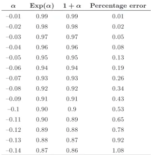
Expanding exponential function in Maclaurin series, keeping the rst two terms, and neglecting the rest, as they have small quantities (see Appendix A), the inventory levels of both products are obtained:

I1(t) = ( b1q1 b3q2 a1)t + q1; 0 t Td1;

(3) I2(t) = ( b2q2 b3q1 a2)t + q2; 0 t Td2:

(4) The inventory level at the end of Tdi is zero; hence,

I(Tdi) = 0. By solving these equations, Tdi is obtained

as:

Td1= _b q1

1q1+ b3q2+ a1; (5)

Figure 1. Inventory levels of the vendor and the buyer for product i.

Td2 =_b q2

2q2+ b3q1+ a2: (6)

The total cost of the supply chain consists of buyer's total cost and vendor's total cost. For each product, the components of the buyer's total cost are as follows: Ordering cost:

Abi

Twi =

Abi

nbinviTdi: (7)

Holding cost at the buyer's warehouse: qihni((nbinvi 1)Tdi (nvi _P1)n_i biqi)

2Tdi : (8)

The average inventory of the buyer's shelf:

Tdi

Z

0

Iidt = qiT₂di: (9)

Buyer's holding cost at shelf: hdiqi

2 : (10)

The cost of transferring items from buyer's warehouse to the shelf:

Si

Tdi: (11)

The components of the vendor's total cost for each product are:

Vendor's set-up cost: Avi

Tvi =

Avi

nvinbiTdi: (12)

Vendor's holding cost: hvinbiqi2

2PiTdi : (13)

Therefore, the system's total prot can be obtained as follows:

T P (q1;q2; nb1; nb2; nv1; nv2) = u_T1q1 d1 +

u2q2

Td2

Av1

nb1nv1Td1

Av2

nb2nv2Td2

Ab1

nb1Td1

Ab2

nb2Td2

S1

Td1

S2

Td2

hv1nb1q12

2P1Td1

hv2nb2q22

2P2Td2

hd1q1

2

hd2q2

2

q1hn1((nb1nv1 1)Td1 (nv1 _P1)n₁ b1q1)

2Td1

q2hn2((nb2nv2 1)Td2 (nv2 _P1)n₂ b2q2)

Substituting Eqs. (5) and (6) into Eq. (14) gives: T P (q1;q2; nb1; nb2; nv1; nv2) = u1(b1q1+ b3q2+ a1)

+ u2(b2q2+ b3q1+ a2)

Av1(b1q1+ b3q2+ a1)

nb1nv1q1

Av2(b2q2+ b3q1+ a2)

nb2nv2q2

hv1nb1q1(b1q1+ b3q2+ a1)

2P1

hv2nb2q2(b2q2+ b3q1+ a2)

2P2

Ab1(b1q1+ b3q2+ a1)

nb1q1

Ab2(b2q2+ b3q1+ a2)

nb2q2

hn1

2 (

(nb1nv1 1)q1

b1q1+ b3q2+ a1

(nv1 1)nb1q1

P1 )(b1q1+ b3q2+ a1)

hn2

2 (

(nb2nv2 1)q2

b2q2+ b3q1+ a2

(nv2 1)nb2q2

P2 )(b2q2+ b3q1+ a2)

S1(b1q1+ b3q2+ a1)

q1

S2(b2q2+ b3q1+ a2)

q2

hd1q1(b1q1+ b3q2+ a1)

2b1q1+ 2b3q2+ 2a1

hd2q2(b2q2+ b3q1+ a2)

2b2q2+ 2b3q1+ 2a2 : ₍₁₅₎

It is desired to nd the optimal solution to the following problem:

Maximize T P (q1; q2; nb1; nb2; nv1; nv2)

Subject to 1 qi Cdi

nbi; nviinteger:

By assuming nvi and nbi as continuous

vari-ables, and taking the second partial derivative of

T P (q1; q2; nb1; nb2; nv1; nv2) with respect to nvi for

given values of qi and nbi, Eq. (16) is obtained:

@2_{T P (n} vi)

@nvi2 =

2Avi

nbin3viTdi: (16)

Taking the second partial derivative of T P (q1; q2;

nb1; nb2; nv1; nv2) with respect to nbi for given values

of qi and nviyields Eq. (17):

@2_{T P (n} bi)

@nbi2 =

2Avi

n3 binviTdi

2Abi

n3

biTdi: (17)

Eq. (16) is negative; thus, T P (q1; q2; nb1; nb2; nv1; nv2)

is a concave function of nvi for given nbi and

qi. Eq. (17) is negative, too; hence, T P (q1; q2; nb1;

nb2; nv1; nv2) is a concave function of nbi for given

values of qi and nvi. The rst partial derivatives of

T P (q1; q2; nb1; nb2; nv1; nv2) with respect to nviand nbi

are taken. By solving:

@T P (q1; q2; nb1; nb2; nv1; nv2)

@nvi = 0;

and:

@T P (q1; q2; nb1; nb2; nv1; nv2)

@nbi = 0:

Eqs. (18) and (19) are obtained as positive roots as shown in Box I.

Using Eqs. (18) and (19), the upper bounds of optimal values of nbi and nvi are obtained. Eq. (18)

shows that there is inverse relation between nvi and

nbi; thus, the maximum value of nvi can be obtained

at nbi = 1. There is not any obvious relation between

nbi or nviand other variables. Thus, to nd the upper

bounds of nvi and nbi, the numerators of Eqs. (18)

and (19) are maximized and their denominators are minimized. Therefore, nvi max and nbi max are

calcu-lated as shown in Box II, where qi min=1, qi max= Cdi,

Tdi max= _bi+bCdi_3+ai and Tdi min= _biCdi+b3C1_{d(3 i)+ai}.

Eq. (20) and Eq. (21) are used in the solution algorithm as upper bounds of the optimum number of shipments to the buyer's warehouse and the optimum number of transferring items from buyer's warehouse to the shelf, respectively.

To nd the optimal solution to Eq. (15), the rst derivative of T P (q1; q2; nb1; nb2; nv1; nv2) is taken with

respect to q1 for given values of nbi and nvi:

@T P (q1; q2; nb1; nb2; nv1; nv2)

@q1 =q

3 1+A_A2

1q 2 1+A_A3

1;₍₂₂₎

where:

A1= b1nb1((nv1 _P1)hn1 hv1)

nvi= p

2qihni(PiTdi qi)AviPi

qihni(PiTdi qi)nbi ; (18)

nbi= p

2Pi(hni(PiTdi qi)nvi+ qi(hni+ hvi))qi(Abinvi+ Avi)nvi

(hni(PiTdi qi)nvi+ qi(hni+ hvi))qinvi : (19)

Box I

nvi max= &p

2qi maxhni(PiTdi max qi max)AviPi qi minhni(PiTdi min qi max)

'

; (20)

nbi max= &p

2Pi(hni(PiTdi max 1)nvi+ qi max(hni+ hvi))qi max(Abinvi+ Avi)nvi max (hni(PiTdi min qi max) + qi min(hni+ hvi))qi min

'

: (21)

Box II

A2=_P 1 1q2P2

1

2b3nb2P1((nv2 1)hn2 hv2)q22

+ P2(( 1₂nv1nb1hn+ u1b1+ u2b3

hd1

2

hn1

2 )P1+ nb1

2 ((nv1 1)hn1 hv1)M1)q2 E2P1P2b3

; A3=

Av1

nb1nv1 +

Ab1

nb1 + S1

M1:

Considering that the signs of A2 and A1 are not

specied, the cubic equation can have zero to three real roots. The possible roots of Eq. (22) are given in Appendix B.

Due to the complexity of the second deriva-tive of T P (q1; q2; nb1; nb2; nv1; nv2) with respect to

qi, it is not possible to prove the convexity of

T P (q1; q2; nb1; nb2; nv1; nv2) in qi. Hence, a heuristic

technique is developed to maximize total prot. Sub-stituting R1, R2, and R3 into Eq. (15), single-variable equations are obtained for given values of nbi and nvi.

Thus, the problem would be to nd the optimum values for these single-variable equations.

4. Algorithm

This section proposes an algorithm to obtain the optimal solution to the problem. The optimal value

of Eq. (15) with six decision variables can be obtained from the following algorithm:

Step 1: Set integer variables of nbi and nviequal to

1 and start with initial values of T Popt_{= 0, n}opt v1 = 0,

nopt_v2 = 0, nb1opt= 0, noptb2 = 0, qopt1 = 0, and q2opt= 0;

Step 2: Set q1 equal to Eq. (B.1); substituting it

into Eq. (15) gives a function of q2, namely, T P (q2).

Take the rst derivative of T P (q2) with respect to q2

and use bi-section method with an initial interval of

[1; Cd2] to nd the optimal value of T P (q2), i.e., q2;

Step 3: Substitute the point obtained from Step 2 into Eq. (B.1) to achieve q

1;

Step 4: Put q

1 and q2obtained in Steps 2 and 3 into

Eq. (15). If T P (q1; q2; nv1; nv2; nb1; nb2) > T Popt;

set TP opt _{= T P (q}

1; q2; nv1; nv2; nb1; nb2), q1opt = q1,

qopt₂ = q2, noptb1 = nb1, noptb2 = nb2, noptv1 = nv1, and

nopt_v2 = nv2. Repeat Steps 2-4 by setting q1 equal to

Eqs. (B.2) and (B.3) and constant values of 1 and 500;

Step 5: Set q1= 1 and q2= Cd2 and put them into

Eq. (15). If T P (q1; q2; nv1; nv2; nb1; nb2) > T Popt,

set T Popt _{= T P (q}

1; q2; nv1; nv2; nb1; nb2), qopt1 = q1,

qopt₂ = q2, noptb1 = nb1, noptb2 = nb2, noptv1 = nv1, and

nopt_v2 = nv2. Repeat this step for q1 = Cd1 and q2 =

Cd2, q1= 1 and q2= 1, and q1= Cd1and q2 = 1;

Step 6: Set nb1= nb1+ 1; if nb1 nmaxb1 , go back to

Step 2;

Step 7: Set nb2= nb2+ 1; if nb2 nmaxb2 , set nb1= 1

Step 8: Set nv1= nv1+1; if nv1 nmaxv1 , set nb1= 1

and nb2= 1 and then go back to Step 2;

Step 9: Set nv2= nv2+1; if nv2 nmaxv2 , set nv1 = 1;

nb1= 1; and nb2= 1 and then go back to Step 2.

5. Numerical study

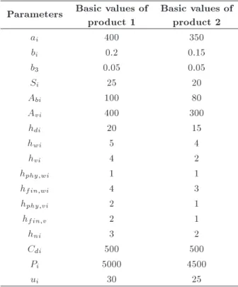
In order to demonstrate the solution procedure nu-merically, an inventory system of two complementary products is studied. Referring to the existing literature, relevant data are chosen and shown in Table 1. When dened parameters change, the changes in the optimal decision values are studied. Tables 2-4 show the compu-tational results. To represent improvement in the total prot, percentage improvement P I is dened as 100 (T P T P0_{)=T P}0_{, where T P}0_{indicates the model prot}

when the complementation rate is ignored. In other words, P I represents protability of the model with two complementary products in comparison with the case where two independent products are concerned.

Figure 2 plots the function T P (q1; q2; nv1; nv2;

n

b1; nb2), where nv1, nv2, nb1, and nb2 are optimal

values.

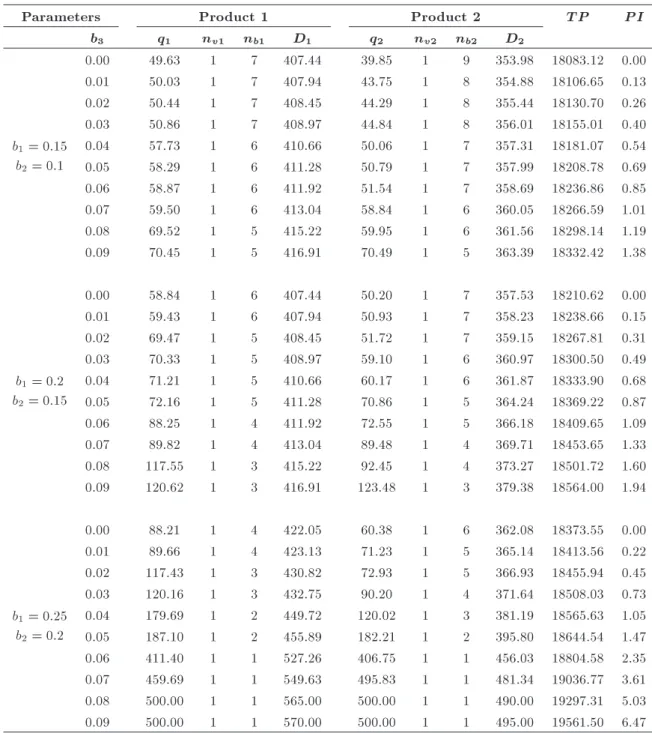
Using the proposed model in Section 3, the eect of complementation rate is studied. Table 2 shows that the complementation rate has signicant eect on the total prot. To analyze the eect of sensitivity of each product to inventory level of the other product, b3,

three levels for parameters, b1 and b2, and nine levels

for parameter b3 are dened. Table 2 indicates that

Table 1. Parameter values in numerical analysis. Parameters Basic values of

product 1

Basic values of product 2

ai 400 350

bi 0.2 0.15

b3 0.05 0.05

Si 25 20

Abi 100 80

Avi 400 300

hdi 20 15

hwi 5 4

hvi 4 2

hphy;wi 1 1

hfin;wi 4 3

hphy;vi 2 1

hfin;v 2 1

hni 3 2

Cdi 500 500

Pi 5000 4500

ui 30 25

Figure 2. Net prot per unit of time as function of q1

and q2.

Figure 3. Eect of b3 on demand (b1= 0:2, b2= 0:15).

when the sensitivity of each product to stock level of its complementary product b3 increases, the quantity

of batch transferred from the warehouse to the shelf of both products qi increases. Furthermore, as b3

increases, the number of transferring lots from buyer's warehouse to shelf of both products nbi decreases.

Hence, when complementation rate of two products is great, the buyer can take advantage of the economy of scale.

It is obvious from Table 2 and Figure 3 that with increasing complementary rate, the demand of product 1 is always greater than that of product 2. This is due to the fact that demand of product 1 is more sensitive to its stock level than that of product 2 is, i.e., b1 > b2. Moreover, as complementation

rate increases, the demand of both products increases, because there is positive relation between demand of a product and stock level of its complementary product. Hence, when the complementation rate increases, as a customer buys one product, he is more likely to buy its complementary product. In other words, ignoring the

Table 2. Sensitivity analysis for parameter b3.

Parameters Product 1 Product 2 T P P I

b3 q1 nv1 nb1 D1 q2 nv2 nb2 D2

b1= 0:15

b2 = 0:1

0.00 49.63 1 7 407.44 39.85 1 9 353.98 18083.12 0.00

0.01 50.03 1 7 407.94 43.75 1 8 354.88 18106.65 0.13

0.02 50.44 1 7 408.45 44.29 1 8 355.44 18130.70 0.26

0.03 50.86 1 7 408.97 44.84 1 8 356.01 18155.01 0.40

0.04 57.73 1 6 410.66 50.06 1 7 357.31 18181.07 0.54

0.05 58.29 1 6 411.28 50.79 1 7 357.99 18208.78 0.69

0.06 58.87 1 6 411.92 51.54 1 7 358.69 18236.86 0.85

0.07 59.50 1 6 413.04 58.84 1 6 360.05 18266.59 1.01

0.08 69.52 1 5 415.22 59.95 1 6 361.56 18298.14 1.19

0.09 70.45 1 5 416.91 70.49 1 5 363.39 18332.42 1.38

b1 = 0:2

b2= 0:15

0.00 58.84 1 6 407.44 50.20 1 7 357.53 18210.62 0.00

0.01 59.43 1 6 407.94 50.93 1 7 358.23 18238.66 0.15

0.02 69.47 1 5 408.45 51.72 1 7 359.15 18267.81 0.31

0.03 70.33 1 5 408.97 59.10 1 6 360.97 18300.50 0.49

0.04 71.21 1 5 410.66 60.17 1 6 361.87 18333.90 0.68

0.05 72.16 1 5 411.28 70.86 1 5 364.24 18369.22 0.87

0.06 88.25 1 4 411.92 72.55 1 5 366.18 18409.65 1.09

0.07 89.82 1 4 413.04 89.48 1 4 369.71 18453.65 1.33

0.08 117.55 1 3 415.22 92.45 1 4 373.27 18501.72 1.60 0.09 120.62 1 3 416.91 123.48 1 3 379.38 18564.00 1.94

b1= 0:25

b2 = 0:2

0.00 88.21 1 4 422.05 60.38 1 6 362.08 18373.55 0.00

0.01 89.66 1 4 423.13 71.23 1 5 365.14 18413.56 0.22

0.02 117.43 1 3 430.82 72.93 1 5 366.93 18455.94 0.45 0.03 120.16 1 3 432.75 90.20 1 4 371.64 18508.03 0.73 0.04 179.69 1 2 449.72 120.02 1 3 381.19 18565.63 1.05 0.05 187.10 1 2 455.89 182.21 1 2 395.80 18644.54 1.47 0.06 411.40 1 1 527.26 406.75 1 1 456.03 18804.58 2.35 0.07 459.69 1 1 549.63 495.83 1 1 481.34 19036.77 3.61 0.08 500.00 1 1 565.00 500.00 1 1 490.00 19297.31 5.03 0.09 500.00 1 1 570.00 500.00 1 1 495.00 19561.50 6.47 complementation between two products leads to the

loss of some customers. Furthermore, Table 2 shows that as sensitivity of both products to their own stock levels bi increases, quantity transferred to the shelf

qi increases and the number of lots transferred from

buyer's warehouse to the shelf nbi decreases. Increase

in bi and qi leads to increase in Di. This is due to

the fact that each product positively depends on its inventory level. Furthermore, increment of bi leads to

increase in the total prot.

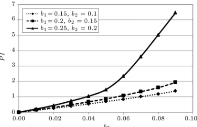
It is obvious from Figure 4 that as complementa-tion rate increases, the value of percentage improve-ment PI increases. Moreover, as sensitivity of each

product to its stock level bi increases, PI increases.

Thus, the prot of selling both products on one retailer shelf is more than the prot of selling them in two dierent retailer stores separately. Furthermore, studying complementary products is more protable when the items are more sensitive to their stock.

It is obvious from Table 3 and Figure 5 that as sensitivity of product 1 to its stock level b1 increases,

q1increases up to b1> 0:26, where capacity constraint

of the rst product is activated, and after that, by increasing b1, q2 is almost constant. Increase in

quantity transferred from buyer's warehouse to the shelf causes higher demand; hence, the prot increases.

Figure 4. Eect of b3 on protability of the proposed

model in comparison with the case that complementation rate is ignored.

Figure 5. Eect of b1 on qi.

When b1 < 0:18, the transferred quantity of product

1, q1, is smaller than that of product 2, q2, because

sensitivity of product 1 to its stock level is smaller than that of product 2 (b1 < b2). Given that product 1

and product 2 are complementary, when b1 increases,

demand of both products increases; however, since complementation rate is small, the increased value is small. Table 3 indicates that demand of product 1 is always more than that of product 2 although the sensitivity of product 1 to its stock level is less than that of product 2 when b1< 0:16.

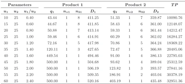
Table 4 shows that when the price of the rst product increases, the transferred quantity of both products increases and their number of transfers de-creases. When the ratio of u1=u2 is smaller than

1.2, although b1 is greater than b2, the transferred

quantity of product 2 is more than that of product 1. For u1=u2> 1:2, q1 signicantly increases until the

capacity constraint of product 1 is activated. In this case, increase in q1 is considerably greater than in q2.

Furthermore, as the quantity transferred to the shelf for both products increases, their demand increases. Hence, increase in u1 leads to increase in total prot.

Thus, study of complementary products with stock-dependent demand is more protable when the items are expensive.

As noted earlier, the following managerial insights can be gained from this paper. Increasing the degree of complementation between two products leads to decrease in the number of transferring batches and increase in transferring size in both vendor and buyer levels. This fact leads to lower supply chain cost. In the other words, considering complementary products helps the supply chain components to benet from the economy of scale. Moreover, displaying complemen-tary products simultaneously on one shelf motivates a buyer, who wants to buy one product, to buy some other products as well. As a result, ignoring comple-mentary relation between products causes decrease in the demand and loss of some customers. Therefore, Table 3. Sensitivity analysis for parameter b1.

Parameters Product 1 Product 2 T P

b1 b2 q1 nv1 nb1 D1 q2 nv2 nb2 D2

0.06 0.15 43.30 1 8 406.13 70.65 1 5 362.76 18154.47

0.08 0.15 44.00 1 8 407.05 70.66 1 5 362.80 18178.79

0.10 0.15 49.35 1 7 408.47 70.70 1 5 363.07 18204.11

0.12 0.15 50.29 1 7 409.57 70.71 1 5 363.12 18231.93

0.14 0.15 57.70 1 6 411.62 70.76 1 5 363.50 18260.91

0.16 0.15 59.05 1 6 412.99 70.77 1 5 363.57 18293.60

0.18 0.15 70.05 1 5 416.15 70.84 1 5 364.13 18329.27

0.20 0.15 72.16 1 5 417.98 70.86 1 5 364.24 18369.22

0.22 0.15 90.26 1 4 423.40 70.97 1 5 365.16 18418.68

0.24 0.15 122.24 1 3 432.90 71.14 1 5 366.78 18482.98

0.26 0.15 409.01 1 1 509.97 72.54 1 5 381.33 18634.65

0.28 0.15 500.00 1 1 543.65 73.01 1 5 385.95 18900.33

0.30 0.15 500.00 1 1 553.65 73.01 1 5 385.95 19187.83

Table 4. Sensitivity analysis for parameter u1.

Parameters Product 1 Product 2 T P

u1 u2 u1=u2 q1 nv1 nb1 D1 q2 nv2 nb2 D2

10 25 0.40 43.44 1 8 411.25 51.33 1 7 359.87 10090.76

15 25 0.60 44.67 1 8 411.85 58.43 1 6 361.00 12148.07

20 25 0.80 50.88 1 7 413.14 59.33 1 6 361.44 14212.47

25 25 1.00 59.46 1 6 414.91 60.29 1 6 362.02 16284.27

30 25 1.20 72.16 1 5 417.98 70.86 1 5 364.24 18369.22

35 25 1.40 120.11 1 3 427.65 72.47 1 5 366.88 20485.06

40 25 1.60 449.54 1 1 494.46 91.00 1 4 386.13 22795.03

45 25 1.80 500.00 1 1 504.68 93.62 1 4 389.04 25312.59

50 25 2.00 500.00 1 1 506.19 123.82 1 3 393.57 27841.16

55 25 2.20 500.00 1 1 509.35 186.91 1 2 403.04 30378.19

60 25 2.40 500.00 1 1 520.16 403.19 1 1 435.48 32951.36

considering the relation between complementary prod-ucts makes increase in the total prot.

This study also shows that when items are more sensitive to stock level, selling of complementary prod-ucts on one retailer shelf leads to more gain. When the sensitivity of one product to its stock level is high, not only the demand of this product, but also the de-mand of other products increases. Hence, considering the relation between complementary products is more crucial when their demand is sensitive to stock. 6. Conclusions

This paper proposed an integrated model for a two-stage supply chain under vendor-managed inventory with consignment stock agreement. The contribution of this paper to the existing literature of consignment stocking policy was considering complementary prod-ucts. Two complementary products were studied and the demand for each product was inuenced not only by its stock level, but also by stock level of the other product. Both of the products were delivered from a vendor to the buyer in equal sizes. The buyer stocked items in the warehouse and on the shelf. Joint total prot of the vendor and the buyer was maximized. A solution algorithm was proposed to nd the optimal transferred quantities and numbers of shipments for both products.

Numerical results showed that increase in sensi-tivity of each product to inventory level of its comple-mentary product would cause increase in the quantity of transfers and decrease in the number of shipments. Hence, the supply chain components could benet from advantages of the economy of scale. Furthermore, considering complementary products could motivate customers to buy more and lead to greater demand. Thus, increase in complementation rate led to increase

in total system prot. The paper also studied the eect of sensitivity of each product to its stock level. The results indicated that when the sensitivity of one product to its inventory level increased, the transferred quantity of both products and, consequently, their demand increased. Analyzing the price of complemen-tary products showed that as the price of one prod-uct increased, the demand of both prodprod-ucts and the total prot increased. Thus, study of complementary products can be more protable when the items are expensive.

The current paper can be extended in the sev-eral directions. The proposed model considered two products. It can be extended to any number of products with dierent complementation rates. Study of substitutable products is another possible exten-sion. The proposed model can also be developed for deteriorating items and other demand functions, e.g., stock- and price-sensitive demands and stochastic demand. Furthermore, multi-vendor multi-buyer is recommended as another topic for future research. References

1. Modak, N.M., Panda, S., and Sana, S.S. \Pricing policy and coordination for a two-layer supply chain of duopolistic retailers and socially responsible manu-facturer", International Journal of Logistics Research and Applications, 19(6), pp. 487-508 (2016).

2. Roy, M.D., Sana, S.S., and Chaudhuri, K. \An inte-grated producer-buyer relationship in the environment of EMQ and JIT production systems", International Journal of Production Research, 50(19), pp. 5597-5614 (2012).

3. Goyal, S.K. \An integrated inventory model for a single supplier-single customer problem", International Journal of Production Research, 15(1), pp. 107-111 (1977).

4. Banerjee, A. \A joint economic-lot-size model for purchaser and vendor", Decision Sciences, 17(3), pp. 292-311 (1986).

5. Goyal, S.K. \A joint economic-lot-size model for pur-chaser and vendor: A comment", Decision Sciences, 19(1), pp. 236-241 (1988).

6. Jokar, M.R.A. and Sajadieh, M.S. \Optimizing a joint economic lot sizing problem with price-sensitive demand", Scientia Iranica. Transactions E, Industrial Engineering, 16(2), pp. 159-164 (2009).

7. Kim, T., Hong, Y., and Chang, S.Y. \Joint economic procurement-production-delivery policy for multiple items in a single-manufacturer, multiple-retailer sys-tem", International Journal of Production Economics, 103(1), pp. 199-208 (2006).

8. Sajadieh, M.S., Jokar, M.R.A., and Modarres, M. \Developing a coordinated vendor-buyer model in two-stage supply chains with stochastic lead-times", Computers and Operations Research, 36(8), pp. 2484-2489 (2009).

9. Ben-Daya, M., Darwish, M., and Ertogral, K. \The joint economic lot sizing problem: Review and ex-tensions", European Journal of Operational Research, 185(2), pp. 726-742 (2008).

10. Glock, C.H. \The joint economic lot size problem: A review", International Journal of Production Eco-nomics, 135(2), pp. 671-686 (2012).

11. Sajadieh, M.S., Thorstenson, A., and Akbari Jokar, M.R. \An integrated vendor-buyer model with stock-dependent demand", Transportation Research Part E: Logistics and Transportation Review, 46(6), pp. 963-974 (2010).

12. Pal, B., Sana, S.S., and Chaudhuri, K. \Joint pricing and ordering policy for two echelon imperfect produc-tion inventory model with two cycles", Internaproduc-tional Journal of Production Economics, 155, pp. 229-238 (2014).

13. Sana, S.S. \Optimal production lot size and reorder point of a two-stage supply chain while random de-mand is sensitive with sales teams' initiatives", Inter-national Journal of Systems Science, 47(2), pp. 450-465 (2014).

14. Sana, S.S. and Panda, S. \Optimal sales team's initiatives and pricing of pharmaceutical products", International Journal of Systems Science: Operations & Logistics, 2(3), pp. 168-176 (2015).

15. Ma, P., Wang, H., and Shang, J. \Supply chain channel strategies with quality and marketing eort-dependent demand", International Journal of Production Eco-nomics, 144(2), pp. 572-581 (2013).

16. Teng, J.T. and Chang, C.T. \Economic production quantity models for deteriorating items with price and stock dependent demand", Computer & Operation Research, 32(2), pp. 297-308 (2005).

17. Goyal, S.K. and Chang, C.T. \Optimal ordering and transfer policy for an inventory with stock dependent demand", European Journal of Operational Research, 196(1), pp. 177-185 (2009).

18. Duan, Y., Li, G., Tien, J.M., and Huo, J. \Inventory models for perishable items with inventory level depen-dent demand rate", Applied Mathematical Modelling, 36(10), pp. 5015-5028 (2012).

19. Yang, S., Hong, K.S., and Lee, C. \Supply chain coordination with stock-dependent demand rate and credit incentives", International Journal of Production Economics, 157(1), pp. 105-111 (2014).

20. Braglia, M. and Zavanella, L. \Modelling an industrial strategy for inventory management in supply chains: the `Consignment Stock' case", International Journal of Production Research, 41(16), pp. 3793-3808 (2003).

21. Yi, H. and Sarker, B.R. \An operational policy for an integrated inventory system under consignment stock policy with controllable lead time and buy-ers' space limitation", Computers and Operations Re-search, 40(11), pp. 2632-2645 (2013).

22. Zanoni, S. and Jaber, M.Y. \A two-level supply chain with consignment stock agreement and stock-dependent demand", International Journal of Produc-tion Research, 53(12), pp. 3561-3572 (2015).

23. Wang, S.P. and Lee, W. \A note on \A two-level supply chain with consignment stock agreement and stock-dependent demand", International Journal of Production Research, 54(9), pp. 2750-2756 (2016).

24. Giri, B.C. and Bardhan, S. \A vendor-buyer JELS model with stock-dependent demand and consigned inventory under buyer's space constraint", Operational Research, 15(1), pp. 79-93 (2015).

25. Hariga, M.A. and Al-Ahmari, A. \An integrated retail space allocation and lot sizing models under vendor managed inventory and consignment stock arrange-ments", Computers and Industrial Engineering, 64(1), pp. 45-55 (2013).

26. Giri, B.C., Bhattachaarjee, R., and Chakraborty, A. \A vendor-buyer integrated inventory system with vendor's capacity constraint", International Journal of Logistics Systems and Management, 21(3), pp. 284-303 (2015).

27. Cardenas-Barron, L.E. and Sana, S.S. \Multi-item EOQ inventory model in a two-layer supply chain while demand varies with promotional eort", Applied Mathematical Modelling, 39(21), pp. 6725-6737 (2015).

28. Ghosh, S.K., Sarkar, T., and Chaudhuri, K. \A multi-item inventory model for deteriorating items in limited storage space with stock-dependent demand", American Journal of Mathematical and Management Sciences, 34(2), pp. 147-161 (2015).

29. Yue, X., Samar K., Mukhopadhyay, S.K., and Zhu, X. \A Bertrand model of pricing of complementary goods under information asymmetry", Journal of Business Research, 59(10), pp. 1182-1192 (2006).

30. Yan, R. and Bandyopadhyay, S. \The prot benets of bundle pricing of complementary products", Journal of Retailing and Consumer Services, 18(4), pp. 355-361 (2011).

31. Wei, J., Zhao, J., and Li, Y. \Pricing decisions for complementary products with rms' dierent market powers", European Journal of Operational Research, 224(3), pp. 507-519 (2013).

32. Taleizadeh, A.A. and Charmchi, M. \Optimal advertis-ing and pricadvertis-ing decisions for complementary products", Journal of Industrial Engineering International, 11(1), pp. 111-117 (2015).

33. Maity, K. and Maiti, M. \Inventory of deteriorating complementary and substitute items with stock depen-dent demand", American Journal of Mathematical and Management Sciences, 25(1-2), pp. 83-96 (2005).

34. Sana, S.S. \An EOQ model for salesmen's initiatives, stock and price sensitive demand of similar products - A dynamical system", Applied Mathematics and Computation, 218(7), pp. 3277-3288 (2011).

35. Stavrulaki, E. \Inventory decisions for substitutable products with stock-dependent demand", Interna-tional Journal of Production Economics, 129(1), pp. 65-78 (2011).

36. Maity, K. and Maiti, M. \Optimal inventory poli-cies for deteriorating complementary and substitute items", International Journal of Systems Science, 40(3), pp. 267-276 (2009).

37. Krommyda, I.P., Skouri, K., and Konstantaras, I. \Op-timal ordering quantities for substitutable products with stock-dependent demand", Applied Mathematical Modelling, 39(1), pp. 147-164 (2015).

Appendix A

Table A.1 shows that the percentage error of applying Maclaurin series is small. Therefore, the third term and higher terms can be neglected.

Table A.1. Absolute percentage error for neglecting the terms higher than 2 in Maclaurin series.

Exp() 1 + Percentage error

{0.01 0.99 0.99 0.01

{0.02 0.98 0.98 0.02

{0.03 0.97 0.97 0.05

{0.04 0.96 0.96 0.08

{0.05 0.95 0.95 0.13

{0.06 0.94 0.94 0.19

{0.07 0.93 0.93 0.26

{0.08 0.92 0.92 0.34

{0.09 0.91 0.91 0.43

{0.1 0.90 0.9 0.53

{0.11 0.90 0.89 0.65

{0.12 0.89 0.88 0.78

{0.13 0.88 0.87 0.92

{0.14 0.87 0.86 1.08

Appendix B

The possible roots of Eq. (22) are:

R1= 1₂((( ((L1q2+ L2+ L3=q2)=A1)6

+729( ((L1q2+ L2+ L3=q2)=3A1)3

((L4q2+ L5)=2A1))2)1=2=27)

((L1q2+ L2+ L3=q2)=3A1)3

(L4q2+ L5)=2A1)1=3

1

2( ((L1q2+ L2+ L3=q2)=3A1)3 ((L4q2+ L5)=2A1)

(( ((L1q2+ L2+ L3=q2)=A1)6

+729( ((L1q2+ L2+ L3=q2)=3A1)3

((L4q2+ L5)=2A1))2)1=2=27))1=3

+1₂( 3(((( ((L1q2+ L2+ L3=q2)=A1)6

+729( ((L1q2+ L2+ L3=q2)=3A1)3

((L4q2+ L5)=2A1))2)1=2=27)

((L1q2+ L2+ L3=q2)=3A1)3

(L4q2+ L5)=2A1)1=3

( ((L1q2+ L2+ L3=q2)=3A1)3

((L4q2+ L5)=2A1)

(( ((L1q2+ L2+ L3=q2)=A1)6

+729( ((L1q2+ L2+ L3=q2)=3A1)3

((L4q2+ L5)=2A1))2)1=2=27))1=3)2)1=2

L1= ( 1

2b3nb2P1((nv2 1)hn2 hv2) +12P2nb1((nv1 1)hn1 hv1)b3) P1P2

L2= (

nv1nb1hn1

2 + u1b1+ u2b3 h2d1 +h2n1)P1+nb1((nv1 1)h2n1 hv1)a1 P1

L3= b3(_nAv2 b2nv2 +

Ab2 nb2 + S2) L4= (_nAv1

b1nv1 + Ab1

nb1 + S1)b3 L5= (_nAv1

b1nv1 + Ab1

nb1 + S1)a1:

Box B.I

R2=(₂₇1 ( ((L1q2+ L2+ L3=q2)=A1)6

+ 729( ((L1q2+ L2+ L3=q2)=3A1)3

(L4q2+ L5)=2A1)2)1=2

((L1q2+ L2+ L3=q2)=3A1)3

(L4q2+ L5)=2A1)1=3

+ ( ((L1q2+ L2+ L3=q2)=3A1)3

(L4q2+ L5)=2A1

(( ((L1q2+ L2+ L3=q2)=A1)6

+ 729( ((L1q2+ L2+ L3=q2)=3A1)3

(L4q2+ L5)=2A1)2)1=2)=27)1=3

(L1q2+ L2+ L3=q2)=3A1; (B.2)

R3= 1₂((( ((L1q2+ L2+ L3=q2)=A1)6

+729( ((L1q2+ L2+ L3=q2)=3A1)3

(L4q2+ L5)=2A1)2)1=2=27)

((L1q2+ L2+ L3=q2)=3A1)3

(L4q2+ L5)=2A1)1=3

1

2( ((L1q2+ L2+ L3=q2)=3A1)3

(L4q2+ L5)=2A1

( ((L1q2+ L2+ L3=q2)=A1)6

+729( ((L1q2+ L2+ L3=q2)=3A1)3

(L4q2+ L5)=2A1)2)1=2=27)1=3

1

2( 3((( ((L1q2+ L2+ L3=q2)=A1)6 +729( ((L1q2+ L2+ L3=q2)=3A1)3

(L4q2+ L5)=2A1)2)1=2=27

((L1q2+ L2+ L3=q2)=3A1)3

(L4q2+ L5)=2A1)1=3

( ((L1q2+ L2+ L3=q2)=3A1)3

(L4q2+ L5)=2A1

( ((L1q2+ L2+ L3=q2)=A1)6

+729( ((L1q2+ L2+ L3=q2)=3A1)3

(L4q2+ L5)=2A1)2)1=2=27)1=3)2)1=2

(L1q2+ L2+ L3=q2)=3A1; (B.3)

L1 to L5 are dened in Box B.I. Expressions (B.1),

Biographies

Mahya Hemmati received her BS degree in Indus-trial Engineering from Isfahan University of Technol-ogy, Isfahan, Iran, in 2014 and her MS degree in Industrial Engineering from Amirkabir University of Technology, Tehran, Iran, in 2016. Her research inter-ests include mathematical optimization, supply chain management, inventory management, and operations research.

Seyyed Mohammad Taghi Fatemi Ghomi was born in Ghom, Iran, on March 11, 1952. He received his BS degree in Industrial Engineering from Sharif University of Technology, Tehran, in 1973 and the PhD degree in Industrial Engineering from University of Bradford, England, in 1980. He worked as planning and control expert in the group of construction and cement industries, a group in the Organization of National Industries of Iran, during the years 1980-1983. Also, he founded the Department of Industrial Training in the aforementioned organization in 1981. He joined Amirkabir University of Technology, Tehran, Iran, as a faculty member in 1983. He is the author

and coauthor of more than 360 technical papers and the author of 6 books on the topics in the area of industrial engineering. His research and teaching interests are in stochastic activity networks, production planning, scheduling, queueing theory, statistical quality control, and time series analysis and forecasting. He is currently professor in the Department of Industrial Engineering at Amirkabir University of Technology, Tehran, Iran, where he was recognized as one of the best researchers of the years 2004 and 2006. He was also recognized as one of the best professors of Iran in the year 2010 by the Ministry of Science and Technology, and in the year 2014 by Amirkabir University of Technology, Tehran, Iran.

Mohsen Sheikh Sajadieh received his PhD degree in Industrial Engineering, in 2009, from Sharif University of Technology, Tehran, Iran. He is now assistant pro-fessor at Amirkabir University of Technology. He is the author and coauthor of more than 30 technical papers and the author of 5 books on the topics in the area of industrial engineering. His research area is focused on supply chain. He is also interested in inventory control, stochastic modeling, and mathematical optimization.