Bayesian Prediction Intervals for Future Order Statistics from the Generalized Exponential Distribution

Vol. 6, No. 1, pp 17-30

Bayesian Prediction Intervals for Future

Order Statistics from the Generalized

Exponential Distribution

Ahmad A. Alamm1, Mohammad Z. Raqab1, Mohamed T. Madi2

1_{Department of Mathematics, University of Jordan, Amman 11942,}

Jordan. ([email protected], [email protected])

2_{Department of Statistics, UAE University, Al Ain, United Arab Emirates.}

([email protected])

Abstract. Let X1, X2, ..., Xr be the first r order statistics from a

sample of size n from the generalized exponential distribution with shape parameter θ. In this paper, we consider a Bayesian approach to predicting future order statistics based on the observed ordered data. The predictive densities are obtained and used to determine prediction intervals for unobserved order statistics for one-sample and two-sample prediction plans. A numerical study is conducted to il-lustrate the prediction procedures.

1

Introduction

LetX1, X2, ..., Xndenote the order statistics of a sample of size n from

generalized exponential (GE) distribution with probability density function (pdf)

f(x;θ) =θ(1−e−x)θ−1e−x; x >0, θ >0. (1)

and cumulative distribution function (cdf)

F(x;θ) = (1−e−x)θ; x >0, θ >0, (2) where θ is a shape parameter. When θ = 1, the GE distribution reduces to the standard exponential distribution. When θ is an in-teger, the GE distribution is the distribution of the maximum of a sample of size n from the standard exponential distribution. The GE distribution has a unique mode and its median is –ln(1-(0.5)1/θ_),

where ln denotes the natural logarithm. Gupta and Kundu (1999) used the above given distribution for analyzing skewed data. Gupta and Kundu (2001a) showed that the GE distribution can be used as a good alternative to the gamma or the Weibull models. They observed that this distribution has more similarities to gamma family than to Weibull family in terms of hazard function. It has an increasing haz-ard function if θ >1 and decreasing hazard function if θ <1. The density function varies significantly depending on the shape parame-ter. Therefore this distribution can also be used in a situation where the course of disease is such that mortality reaches a peak after some finite period, and then slowly decline. For example, in a study of cur-ability of breast cancer, Langlands et al. (1979) found that the peak of mortality occurred after three years. It is therefore, important to analyze such data sets with appropriate models like gamma, Weibull or GE distributions. The GE distribution has many properties that are quite similar to those of the gamma distribution, but it has a dis-tribution function similar to that of the Weibull disdis-tribution which can be computed simply. The GE family has likelihood ratio order-ing on the shape parameter; so it is possible to construct uniformly most powerful test for testing one-sided hypothesis on the shape pa-rameter, when the scale and location parameters are known. Gupta and Kundu (2003) used the ratio of the maximized likelihoods in dis-criminating between the Weibull and the GE distributions. Raqab and Ahsanullah (2001) and Raqab (2002) obtained the estimation of the location and scale parameters of the GE distributions based on order statistics and record values, respectively. Recently Raqab and Madi (2005) used importance sampling techniques in the Bayesian estimation and prediction for the GE distribution.

Let X1, X2, ..., Xn be the order statistics from a sample of size

n from GE distribution. Let X = (X1, X2, ..., Xr), r ≤ n, be the

censored sample. Prediction problem does arise naturally in the con-text of order statistics. Two prediction scenarios are considered; first,

given the r observed order statistics x1 ≤x2 ≤... ≤xr, we predict

the remaining order statistics xr+1, xr+2, ..., xn. This is referred to

as one-sample prediction. The second scenario, known as the two-sample prediction, consists of predicting the first m order statistics in a future sample. Prediction intervals for different statistics of fu-ture observations are discussed in the literafu-ture. Ahsanullah (1980) developed the best linear unbiased predictors (BLUP’s) of the future record statistics from the exponential distribution. Raqab (1997) ob-tained the modified maximum likelihood predictors of future order statistics from normal samples. Other prediction problems can be found in Lawless (1973), Kaminsky and Nelson (1974), Evans and Ragab (1983) and Sartawi and Abu-Salih (1991).

In the context of prediction, we say that (L(X), U(X)) is a 100(1− α)% prediction interval for a future random variableY if

P(L(X)< Y < U(X)) = 1−α,

whereL(X) and U(X) are lower and upper prediction limits for the random variable Y, and 1 −α is called the confidence prediction coefficient.

In this paper, we use Bayesian statistical analysis to predict fu-ture order statistics from GE distribution on the basis of some ordered data. In Section 2, we obtain prediction intervals for order statistics using a one-sample prediction plan. In Section 3, we present predic-tion intervals for future order data based on a two-sample predicpredic-tion plan. Section 4 includes an illustration of the proposed methods using a simulated data set and different choices of prior parameters.

2

Bayesian Prediction Interval for the

(

r

+

s

)

Order Statistic: One-Sample Case

The likelihood forθof the given type II censored sampleX= (X1, X2, . . . , Xr) is given by:

f(x|θ) =

n! (n−r)!θ

r r Y i=1

e−xi

r Y i=1

(1−e−xi₎θ−1h_{1− 1−e}−xrθin−r ₍₃₎

0≤x1 ≤...≤xr, θ >0.

We assume that θ follows a Gamma distribution with density function

π(θ) = b

a

Γ(a)θ

a−1_e−bθ_{, θ >0. (4)}

From (3) and (4), we get the posterior density of θ as

π(θ|x) = θ

a+r−1_e−bθ_vθ_(1−ωθ₎n−r Pn−r

k=0

n−r k

(−1)k_(b−ln(ωk_v))−a−r _Γ(a+r), (5)

where

v=

r Y i=1

(1−e−xi_{) andω= 1−e}−xr_.

Let Xr+1,Xr+2,..., Xn be the future remaining order statistics.

The extended likelihood function is

f(x1, x2, .., xr+s, .., xn|θ) = n!f(x1|θ)...f(xr+s|θ)...f(xn|θ),

0≤x1 ≤...≤xr≤...≤xn (6)

By integrating (6), with respectxr+1, xr+2, .., xr+s−1, xr+s+1.., xn,

we have

f(x1, x2, .., xr, xr+s|θ) =

n!

(s−1)!(n−s−r)!

r Y i=1

f(xi)[F(xr+s)−F(xr)]s−1

[1−F(xr+s)]n−r−s f(xr+s). (7)

On using (1) and (2), we obtain

f(x1, x2, .., xr, xr+s|θ) =

n!

(s−1)!(n−s−r)!θ

r+1

r Y i=1

h

e−xi_(1−e−xi₎θ−1i

h

exr+s_(1−e−xr+s₎θ−1i h_1−(1−e−xr+s₎θin−r−s

s−1

X i=1

(−1)i

i!(s−i−1)!(1−e

−xr₎θi_(1−e−xr+s₎θ(s−i−1) ₍₈₎

It follows from (3) and (8) that

f(xr+s|θ,x) =

s n−r s

!

θhe−xr+s_(1−e−xr+s₎θ−1i

h

1−(1−e−xr+s₎θin−r−s_(1−ωθ₎r−n

s−1

X i=0

(−1)i s−1

i

!

(1−e−xi₎θi_(1−e−xr+s₎θ(s−i−1) ₍₉₎

Forming the product of f(xr+s|θ,x) and the posterior density

of θ given in (5) and integrating out θ, it may be shown that for 1≤s≤n−r, the predictive density function of xr+s givenx is

p(xr+s|x) =

s n−_sr

e−xr+sPs−1

i=0

Pn−r−s

j=0 (−1)i+j s −1

i

n−r−s j

Wij Pn−r

k=0

n−r k

(−1)k_(b−ln(ωk_v))−a−r

Γ(a+r) ,

xr+s>0, (10)

where

Wij =

(1−e−xr+s₎−1_{Γ(a+r+ 1)}

b−ln

v ωi_(1−e−xr+s₎(j+s−i) a+r+1

.

The predictive densityp(xr+s|x) can be used to find the prediction

bounds on xr+s. Note that

P(Xr+s≥y|x) =

s n−_sr

T

s−1

X i=0

n−r−s X j=0

(−1)i+j s−_i1 n−r−s j

(j−i+s)

[b−ln(ωiv)]−(a+r)

 



1−

"

1−(j−i+s) ln(1−e −y) b−ln(ωi _v)

#−(a+r) 



(11)

where

T =

n−r X

k=0

n−r k

!

(−1)k(b−ln(ωk v))−(a+r).

LetL(x) andU(x) be the lower and upper bounds for 100(1−α)% prediction interval, respectively. Then 100(1−α)% prediction bounds can be obtained by equating (11) to 1−α/2 for the lower limit and

α/2 for the upper limit and solving the resulting equations for y using numerical techniques.

When s= 1 (we wish to predict the next failure time), Equation (11) becomes

P(Xr+1≥y|x) = n−r

T

n−r−1

X j=0

(−1)j n−r_j−j

(j−i+s) [b−ln(v)]

−(a+r)

 



1−

"

1− (j+ 1) ln(1−e −y₎

b−ln(v)

#−(a+r) 



. (12)

When s=n−r ; that is, we predict the last failure time. In this case, Equation (11) reduces to

P(Xn≥y|x) =

n−r T

n−r−1

X i=0

(−1)i n−r_i−1

(i+n−r)

h

b−ln(ωiv)i−(a+r)

 



1−

"

1−(n−r−i) ln(1−e −y₎

b−ln(ωi_v)

#−(a+r) 



. (13)

from which prediction can be made about Xn. Consider the special

case where r = n−1, and s = 1. In this case, we predict the last failure time Xn based on observing X1, X2, ..., Xn−1. Substituting r=n−1 in (13) and solving the equation:

P(Xn≥y|x) =γ, (14)

where γ = 1−α/2 and γ = α/2, we get a 100(1−α)% prediction interval forXn as (L(x), U(x)),so that

L(x) =−ln



1−

eb v

!ξ1

 and U(x) =−ln 

1−

eb v

!ξ2

,

where

ξ1 = 1−



1−

1 1−c1+₂α



 1 r+a

,

and

ξ2 = 1−



1−

1 1−c1−₂α



 1 r+a

,

with

c= 1−

1− ln(ω) b−ln(v)

−(r+a)

.

Prediction intervals for the remaining order statistics can also be found using The Gibbs Sampler. Let Z = (Xr+1,Xr+2,..., Xn). By

forming the product of the extended likelihood and the prior of θ, the full Bayesian model is expressed as

π(θ,z|x)∝θn+a−1exp{ −nx−θ(D+b) +D},

whereD=−Pn

i=1ln(1−e−xi) andx=Pni=1xi/n.

Setting Zs = (Xr+1, ..., Xs−1, Xs+1, ...Xn), the full conditional

distribution of Xs (r+ 1≤s≤n),is found to be

π(xs|x,zs, θ) =     

   

θe−xs_(1−e−xs₎θ−1_I[x

s−1<xs<xs+1]

(1−e−xs+1₎θ_−(1−e−_xs−1

)θ , s=r+ 1, ..., n−1

θe−xn_(1−e−xn₎θ−1_I

(_xn>xn−1)

1−(1−e−xn−1₎θ , s=n.

(15) and the full conditional distribution ofθ|x,y is G(n+a, D+b).

Given an arbitrary set of starting values of θ and z, we gener-ate values from (15) using the inverse cdf transformation method (Devroye, 1986) as follows:

Xj=−ln

n

1−

(1−e−Xj−1₎θ_+U(1−e−Xj+1₎θ_−(1−e−Xj−1₎θθ

−1o

, f or j=r+ 1, ..., n−1,

Xn=−ln

n

1−

(1−e−Xj−1₎θ_+U1−(1−e−Xn−1₎θθ

−1o

(16) whereU ∼U(0,1). In fact, θis generated directly from its standard full conditional distribution.

3

Bayesian Prediction Interval for Future

order Statistics: Two-Sample Case

LetY= (Y1, Y2, ..., Ym) be a future ordered random sample

indepen-dent ofXfrom the GE distribution with density (3). It can be shown

that the predictive density ofYk given xis expressed as

p(yk|x) =

k m_k

e−yk_(1−e−yk₎−1Pn−r

i=0

Pm−k j=0

n−r i

m−k j

(−1)i+j Vij

Q(x) where

Q(x) =

n−r X

k=0

n−r k

!

(−1)k(b−ln(ωkv))−a−r Γ(a+r)

and

V = Γ(a+r+ 1)

{b−ln [ωi _v(1−e−yk)k+j]}a+r+1

It follows that

P(Yk ≥ y|x) =

k m_k

T

n−r X

i=0

m−k X

j=0

n−r i

m−k j

(−1)i+j[b−ln(ωiv)]−a−r (k+j)

.    1− "

1−(k+j) ln(1−e −y₎

b−ln(ωk_v)

#−a−r 



, (17)

where

T =

n−r X

k=0

n−r k

!

(−1)k[b−ln(ωiv)]−a−r.

Since (17) does not permit explicit solution for the prediction bounds on yk,numerical methods have to be employed. The 100(1−

α)% prediction bounds for thekth order statisticYkcan be obtained

by equating (17) to 1−α/2 for the lower limit and α/2 for the up-per limit and solving the resulting equations for y using numerical techniques.

For example, to predict Ym,we need to solve

1−1 T

n−r X i=0

n−r i

!

(−1)i[(b−ln(ωi v))−mln(1−e−y)]−a−r=γ (18)

and if r = n (prediction of Ym based on a complete sample), (18)

reduces to

1−

"

1−mln(1−e −y₎

b−lnv

#−a−n

=γ

and results in

L(x) =−ln



1−

eb v

!δ1

 and U(x) =−ln 

1−

eb v

!δ2

,

where

δ1 =m−1[1−(

2 2−α)

1

a+n and δ₂= 1−(2

α)

1 a+n.

Whenr=nandk= 1,we predictY1based on a complete sample

of size n.Then we have to solve

m

m−1

X j=0

m−1

j

(−1)j (1 +j)

 



1−

"

1−(1 +j) ln(1−e −y₎

b−lnv

#−a−n 



=γ (19)

A special case of (19) is to predict a single future failure. Setting

m= 1 in (19), we get

1−

"

1− ln(1−e −y₎

b−lnv

#−a−n

=γ.

The resulting 100(1−α)% prediction limits are

L(x) =−ln

"

1− e

b

v

!κ1#

and U(x) =−ln

"

1− e

b

v

!κ2#

.

where

κ1 = 1−(

2

α)

1

a+n _{and κ}

2= 1−(

2 2−α)

1 a+n_.

Prediction intervals for the future order statistics can also be found via MCMC. By forming the product of the extended likeli-hood and the prior of θ, the full Bayesian model is expressed as

π(θ,y|x) ∝ θm+r+a−1exp{ −my−θ(Dm+b) +Dm} n−r

X i=0

n−r i

!

(−1)iexp{−θ[Dr+iTr]},

where Dm =−Pmi=1ln(1−e−yi), y =Pmi=1yi/m, Dr =− r P i=1

ln(1− e−xi_{) and T}

r =−ln(1−e−xr).

SettingYk= (Y1, ..., Yk−1, Yk+1, ...Ym),the full conditional

distri-bution ofYk (1≤k≤m),is found to be

π(yk|x,yk, θ) =         

θ e−yk(1−e−yk)θ−1_I[y

k−1<yk<yk+1]

(1−e−yk+1₎θ_−(1−e−yk−1₎θ , k= 1, ..., m−1

θe−ym (1−e−ym)θ−1_I

(_{ym >ym}−1)

1−(1−e−ym−1₎θ , k=m,

(20)

and the full conditional distribution ofθ|x,y is given by

π(θ|x,y)∝θm+r+a−1

n−r X i=0

n−r i

!

(−1)iexp{−θ[Dr+Dm+iTr+b]}

Using the Gibbs sampler to estimate the posterior distribution requires being able to sample from the full conditional distributions for each quantity involved. This is the case for Yk but not for

θ.Consequently, Metropolis-Hastings (M-H) steps are introduced into the Gibbs sampler so that Yk is sampled directly from its full

con-ditional distribution via the the inverse cdf transformation method, whereasθ is updated via a M-H step as explained in Tierney (1994), usingG(m+r+a, Dr+Dm+b) as a proposal distribution.The M-H

step proceeds as follows: Given θ(i−1),

(i) Sampley from G[m+r+a, Dr+Dm+b] and u from U(0,1)

(ii) If u <min(1, ϑ) then letθ(i)_{=y else go to (i), where}

ϑ=

Pn−r i=0(−1)i(

n−r i )e

−(iyTr)

Pn−r i=0(−1)i(

n−r

i )e−(iθTr)

.

4

Data Analysis

In this section, we illustrate the procedures by presenting a complete analysis for a simulated data set. The following data sample was gen-erated from GE distribution G(3, 1). Suppose that r = 15 observed order statistics are available from a sample of size n= 20.These ob-servations are as follows:

0.65306, 0.67631, 0.68341, 1.05645, 1.46194, 1.71555, 1.73903, 1.78940, 1.79847, 1.82522, 1.95587, 2.16530, 2.35033, 2.38706, 2.39005

We present some results to compare the performance of the classi-cal and Bayesian approaches for different choices of prior parameters. All computations are performed via Mathematica 5.0 and Fortran-90. We use the iterative alogirthm to find the root y that solves

P(Xr+s > y) = γ = 0.975 and γ = 0.025 and the iterative

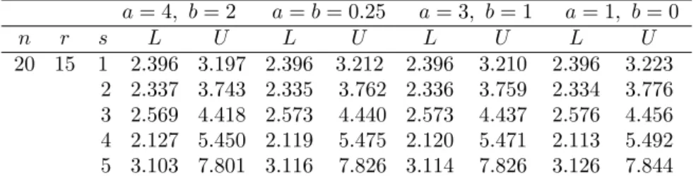
pro-cess stops when the difference between two consecutive iterates are less than 10−10. This allows us to compute 95% confidence inter-vals. Tables 1 and 3 present 95% Bayesian prediction intervals of

Xi(i = 16,17, ...,20) and Yi(i = 1,2, ...,5) for prior parameters

(a= 4, b= 2), (a=b= 0.25), (a = 3, b= 1) and (a= 1, b = 0).

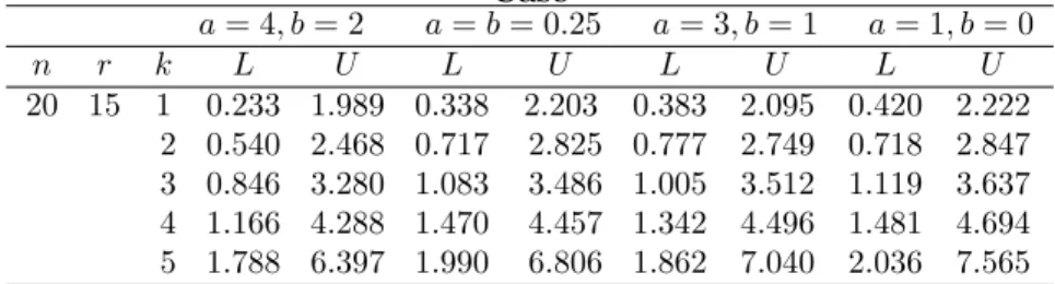
Further, we apply the Gibbs and Metropolis samplers to determine the Bayesian prediction intervals. After setting initial values of θ

and x for the one-sample prediction and θ and y for the 2-sample prediction, a sampler single chain with pre-determined number of iterations is run and used as input in Raftery & Lewis Fortran pro-gram (Raftery and Lewis, 1992) to determine the required number of iterations needed to attain convergence. Subsequent to conver-gence, 5,000 draws of equally spaced variates were collected for the parameterθ as well asx andy. Tables 2 and 4 present 95% MCMC prediction intervals for the remaining and future order statistics.

Although, both mehods provide close lower and upper limits of 95% prediction intervals, it is observed that the prediction intervals tend be wider when s and k increase. This is a natural, since the prediction of the future order statistic that is far a way from the last observed value has less accuracy than that of other future order statistics.

Table 1: Bayesian Prediction Intervals:One-Sample Case

a= 4, b= 2 a=b= 0.25 a= 3, b= 1 a= 1, b= 0

n r s L U L U L U L U

20 15 1 2.396 3.197 2.396 3.212 2.396 3.210 2.396 3.223 2 2.337 3.743 2.335 3.762 2.336 3.759 2.334 3.776 3 2.569 4.418 2.573 4.440 2.573 4.437 2.576 4.456 4 2.127 5.450 2.119 5.475 2.120 5.471 2.113 5.492 5 3.103 7.801 3.116 7.826 3.114 7.826 3.126 7.844 Table 2: MCMC Bayesian Prediction Intervals: One-Sample Case

a= 4, b= 2 a=b= 0.25 a= 3, b= 1 a= 1, b= 0

n r s L U L U L U L U

20 15 1 2.397 3.184 2.396 3.209 2.396 3.210 2.396 3.212 2 2.452 3.752 2.457 3.792 2.458 3.741 2.456 3.757 3 2.566 4.442 2.575 4.447 2.577 4.444 2.572 4.461 4 2.764 5.474 2.773 5.503 2.755 5.524 2.758 5.503 5 3.113 7.994 3.127 7.954 3.088 7.968 3.112 7.891

Table 3: Bayesian Prediction Intervals: Two-Sample Case

a= 4, b= 2 a=b= 0.25 a= 3, b= 1 a= 1, b= 0

n r k L U L U L U L U

20 15 1 0.222 1.854 0.273 1.991 0.273 1.969 0.318 2.073 2 0.521 2.475 0.597 2.617 0.596 2.595 0.661 2.702 3 0.815 3.187 0.906 3.324 0.904 3.309 0.979 3.417 4 1.153 4.235 1.255 4.377 1.252 4.357 1.335 4.466 5 1.630 6.582 1.743 6.723 1.738 6.705 1.828 6.813

Table 4: MCMC Bayesian Prediction Intervals: Two-Sample Case

a= 4, b= 2 a=b= 0.25 a= 3, b= 1 a= 1, b= 0

n r k L U L U L U L U

20 15 1 0.233 1.989 0.338 2.203 0.383 2.095 0.420 2.222 2 0.540 2.468 0.717 2.825 0.777 2.749 0.718 2.847 3 0.846 3.280 1.083 3.486 1.005 3.512 1.119 3.637 4 1.166 4.288 1.470 4.457 1.342 4.496 1.481 4.694 5 1.788 6.397 1.990 6.806 1.862 7.040 2.036 7.565

Acknowledgements

The authors are thankful to the referees for their valuable comments that improved on the original version of the manuscript.

References

Ahsanullah, M. (1980), Linear prediction of record values for the two parameter exponential distribution. Annals of the Institute of Statistical Mathematics, 32, 363-368.

Arnold, B. C., Balakrishnan, N., and Nagaraja, H. N. (1992), A first Course in Order Statistics. New York: Wiley.

Devroye, L. (1986), Non-Uniform Random Variates Generation. Ber-lin: Springer-Verlag.

Evans, I. G. and Ragab, A. S. (1983), Bayesian inferences given a type 2 censored sample from a burr distribution. Communica-tions in Statistics-Theory and Methods, 12, 1569-1580.

Gupta, R. D. and Kundu, D. (1999), Generalized exponential dis-tribution. Austral. N. Z. Statist., 41(2), 173-188.

Gupta, R. D. and Kundu, D. (2001a), Exponentiated exponential distribution, an alternative to gamma and weibull distributions. Biometrical J., 43(1), 117-130.

Gupta, R. D. and Kundu, D. (2001b), Generalized exponential dis-tributions: different methods of estimation. J. Statist. Com-put. Simulations, 69(4), 315-338.

Gupta, R. D. and Kundu, D. (2003), Discriminating between weibull and generalized exponential distributions. Computational Statis-tics and Data Analysis, 43, 179-196.

Kaminsky, K. S. and Nelson, P. I. (1974), Prediction intervals for the exponential distribution using subsets of the data. Techno-metrics,16, 57-59.

Langlands, A. O., Pocock, S. J., Kerr, G. R., and Gore, S. M. (1979), Long term survival of patients with breast cancer: a study of curability of the disease. Brit. Med. J.,2, 1247-1251.

Lawless, J. F. (1973), On estimation of safe life when the underlying life distribution is weibull. Technometrics, 15(4), 857-865. Kundu, D. and Gupta, R. D. (2005), Estimation of P(Y < X) for

generalized exponential distribution. Metrika,61(3), 291-308. Kotz, S., Lumelskii, Y., and Pensky, M. (2003), The Stress-Strength

Model and its Generalizations. New York: World Scientific. Lawless, J. F. (1982), Statistical Models and Methods for Lifetime

Data. New York: Wiley.

Raftery, A. E. and Lewis, S. (1992), How many iterations in the gibbs sampler? Bayesian Statistics, 4, Eds. Bernardo, J. M., Berger, J., Dawid, A. P., and Smith, A. F. M., Oxford, UK, 763-773.

Raqab, M. Z. (1997), Modified maximum likelihood predictors of future order statistics from normal samples. Computational Statistics and Data Analysis, 25, 91-106.

Raqab, M. Z. (2002), Inferences for generalized exponential distribu-tion based on record statistics. Journal of Statistical Planning and Inference,104(2), 339-350.

Raqab, M. Z. and Ahsanullah, M. (2001), Estimation of location and scale parameters of generalized exponential distribution based on order statistics. Journal of Statistical Computation and Sim-ulation,69(2), 109-124.

Raqab, M. Z. and Madi, M. T. (2005), Bayesian inference for the generalized exponential distribution. Journal of Statistical Com-putation and Simulation,69(2), 109-124.

Sartawi, H. A. Abu-Salih, M. S. (1991), Bayesian prediction bounds for the burr type X model. Communications in Statistics-Theory and Methods, 20(7), 2307-2330.

Tierney, L. (1994), Markov chains for exploring posterior distribu-tions. Annals of Statistics, 22, 1701-1762.