151
Measuring performance of a three-stage structure using data
envelopment analysis and Stackelberg game
Ehsan Vaezi
1, Seyyed Esmaeil Najafi
1*, Seyyed Mohammad Hajimolana
1, Farhad
Hosseinzadeh Lotfi
2, Mahnaz Ahadzadeh Namin
31Department of Industrial Engineering,Science and Research Branch, Islamic Azad University, Tehran, Iran
2Department of Mathematics,Science and Research Branch, Islamic Azad University, Tehran, Iran 3Department of Mathematics, Shahr.e Qods Branch, Islamic Azad University, Tehran, Iran
[email protected], [email protected], [email protected], [email protected], [email protected]
Abstract
In this paper, we consider a three-stage network comprised of a leader and two followers in respect to the additional desirable and undesirable inputs and outputs. We utilize the non-cooperative approach multiplicative model to measure the efficiency of the overall system and the performances of decision-making units (DMUs) from both, the optimistic and pessimistic views. Moreover, we utilize the concept of a goal programming and define a kind of cooperation between the leader and followers, so that the objectives of the managers are capable of being inserted in the models. In actual fact, a kind of collaboration is considered in a non-cooperative game. The non-cooperative models from this view cannot be converted into linear models. Therefore, a heuristic method is proposed to convert the nonlinear models into linear models. After obtaining the efficiencies based on the double-frontier view, the DMUs are ranked and classified into three clusters by the k-means algorithm. Finally, this paper considers a genuine world example, in relevance to production planning and inventory control, for model application and analyzes it from the double-frontier view. The proposed models are simulations of a factory in a real world, with a production area as leader and a warehouse and a delivery point as two followers. This factory has been regarded as a dynamic network with a time period of 24 intervals.
Keywords: Network DEA, game theory, Stackelberg game, goal programming, double-frontier, undesirable output.
1- Introduction
Evaluation and the measurement of performance lead to smart or intelligent systems with incentives for individuals for the desired behavior. Performance measurement is one of the fundamental managerial processes, for analyzing their own performance and likewise, surveying the conformity between the performance and the set of goals. The outcome of the evaluation can provide the grounds for taking the correct measures in decision-making for the future. Performance appraisal is a key part in the formulation and implementation of organizational policies.
*Corresponding author
ISSN: 1735-8272, Copyright c 2019 JISE. All rights reserved
Journal of Industrial and Systems Engineering
Vol. 12, No. 2, pp. 151-173 Spring (April) 2019
152
Today, all organizations have somehow, depicted the importance, of having a measuring system, for performance. As a principle, every organization should and till wherever feasible, measure its performance capacities.
The absence of an effective assessment or evaluation system is directly related to the disintegration of an organization and this shortcoming is considered an organizational disease; for without measuring, there shall be no basis for judgments, opinions and evaluations. As whatever cannot be evaluated, cannot be even fittingly managed. So as to ensure a correct management, every organization must use scientific models for the evaluation of performance, so that its efforts and the results achieved from its performance can be appraised. Several factors have an impact on the growth and development of countries. Researches executed in this arena indicate that efficiency impacts enhance the speed of economic development. These surveys have revealed that in the past years, there is a difference in the economic growth and development of countries due to modification in the level of efficiency and productivity of factors relative to production. Thence, an increment in performance and efficiency of organizations is an inevitable necessity, for survival, in global markets today. This issue is not confined to a particular sector or industry and in a limited period of time shall encompass all the sectors of economy. A performance assessment is a process which appraises measures, evaluates and judges the performance of an organization during a given period. This measuring of performance is carried out by comparing the present circumstances with that of the desirable or ideal conditions, which are based on pre-determined indexes. In general, the objectives of assessing the performance are a response to the results in specifying quality improvement measures and to reduce costs, as well as comprehend, as to what is being evaluated. The performance evaluation topics can be examined from different views. There are two traditional and modern views in this regard. The traditional view focuses solely on the work of the past period and is shaped by the requirements of the past. In this view, the time and space conditions of the system are ignored and may cause deviations as a result of work. A new view has targeted education, growth and development of evaluated capacities and performance improvements. This approach identifies the weaknesses and strengths of the systems. In the new view, the problem is studied in the context of time and a systemic attitude is dominant. Organizational units are only a part of the whole system. As a result, a new view leads to growth and development, improvement of performance, and the realization of the goals of the organization. In recent years, several models and approaches have been proposed for measuring efficiency, based on two general parametric and non-parametric methods. In this research, the Data Envelopment Analysis (DEA) is used as a nonparametric approach. This method selects the efficient units and provides the efficiency frontier. This frontier is a criterion for the evaluation of other units. In this paper, we will measure the performance by using the data envelopment analysis method for the following five reasons. First, it evaluates the performance of the organization on the basis of a logical model with a flexible structure. Second, it detects inefficient units. Third, the degree of inefficiency of the units is determined. Fourth, there is no prior standard level and the comparison criterion is another unit that operates under the same conditions. Fifth, DEA determines the patterns and references for the inefficient units among of the efficient units.
The DEA is a theoretical framework which discusses the analyzing of efficiency and its application in the arena of production planning and inventory control is observed very poorly. In the past two decades, the manufacturing or production sector has grown significantly and being attentive towards production is one of the key goals of Iran’s programs. An increment in the importance of the production sector, during the recent years and anxiety as to efficiency growth in this sphere, has a direct correlation with the economic system. A rise in costs, has led to pressurizing the production units to increase their organizational efficiency. A rise in costs, has led to haul, the production units towards incrementing their organizational performance. The best manner to ensure an efficiency increase would be to carry out a correct and logical use of the resources available. This could only be accomplished by ensuring a correct managerial performance, including a coherent evaluation of the returns attained.In continuation, the paper unfolds as follows:Section (2) reviews the literature on the data envelopment analysis approach. Section (3), describes the methodology and model formulation. In section (4), the heuristic approach has been described, so as to resolve the non-cooperative view of the network analysis. Section (5) of the paper describes a factory, evaluating it dynamically and section (6) concludes the paper.
153
2- Literature review
Data Envelopment Analysis (DEA) is a non-parametric method for measuring the relative efficiency of a set of analogous decision-making units (DMUs), with multiple inputs and outputs (Hwang et al., 2013). This method is considered a frontier or boundary function surrounding and involving the input and output factors. It not only determines the most efficient units, but it also analyses the inefficient ones (Kritikos, 2017). Charnes et al. (1978) developed the initial DEA task of Farrel (1957), the said model was known as (Charnes-Cooper Rhodes) or the “CCR Model”. Banker et al. (1984) expanded the DEA models and presented the (Banker-Charnes-Cooper) or the “BCC Model”. The classical data envelopment analysis models, such as, the CCR and BCC, assume that the systems are considered as black boxes; and due to the shortcomings in considering the intermediary variables and the internal interactions of the system, valuable information is eliminated (Lee et al., 2016). Fare and Grosskopf (2000) indicated to the disadvantages and weak points of the classical DEA models and referred to the Network Data Envelopment Analysis Model (NDEA). These models defined the interactions and intermediate variables and similarly, by utilizing the series and parallel sub-divisions, dealt with evaluating the efficiency of complex systems. Since the NDEA Models take into account the internal interactions of systems, hence, a more realistic performance of the systems can be demonstrated. In network models the performance of the entire system is calculated in relevance to the constraints or restrictions of the internal processes and the interactions between the general efficiency and that of the processes is established. Though, in the classic DEA Models, if the DMU has internal processes, the efficiency of these internal processes and the general process is computed independently and the correlations between the general efficiency and that of the processes is not conventional (Chen & Yan, 2011). Kao (2009) categorized the network models into three sets, namely, series, parallel and hybrid. Kao stated that, when activities in a system are protracted in respect to each other, the system is of a series structure; and whenever activities are in a parallel form alongside each other, the system has a parallel structure. Similarly, when there is a hybrid condition between the series and parallel aspects, a hybrid mode is engaged. In order to calculate the efficiency of the entire network, both, in the series or parallel mode, usually, the efficiency coefficient attained in the stages relative to each other and the weighted average efficiency or the stages are normally and respectively utilized. In a series or parallel structure, a DMU is efficient when all its sub-processes are efficient (Kou et al., 2016). Several studies have been carried out in relevance to NDEA and in respect to which, the task of Cook et al. (2010) can be indicted. They developed a multi-stage model, in which each stage is able to consider the additional inputs and outputs. In fact, in this model, the outputs of each stage can be regarded as the final product and exit the system and or enter the next stage as an input. Thereby, each stage can take the additional inputs into consideration, as not being the outputs of the prior stage. Zhou et al. (2018), review the literature on network data envelopment analysis (NDEA) applications in sustainability using citation-based approaches from 1996 to 2016. In the past few years, in relevance to network analysis, new discussions have been contributed in view of the game theory, such that this theory has become one of the vital methods in the analysis of NDEA or have been converted into multi-stage models (Liang et al., 2008). Li et al. (2012) rendered a model for a two-stage structure, a phase of which holds a more important standpoint for managers. They have named this phase as “leader” and the other phase as “follower”. In order to calculate the efficiency, initially, the efficiency of the leader phase was maximized to the optimum and then the efficiency of the follower phase was brought to hand, by maintaining a constant efficiency for the leader phase. This model was known as a decentralized controlled or a Stackelberg game, which has been widely used by researchers in the recent years. An et al. (2017), took a network, comprising of two stages with a collaborative condition between them into consideration and computed the efficiency of this network in the cooperative and non-cooperative conditions on a (leader-follower) basis. The results demonstrated that, the overall efficiency in cooperative conditions was higher than that of the non-cooperative one. Wu et al. (2016) contemplated on and computed the efficiency of a two-stage network, in another similar research, with undesirable outputs in cooperative and non-cooperative conditions. The results of this research, which considers the total efficiency as the sum of the efficiency component, denotes that, the efficiency of the sub-DMUs is in the condition of a leader in the maximal and as a follower in the minimal. In yet another research by Zhou et al. (2018), a network consisting of a leader and some followers were evaluated in a black box and non-cooperative modes
154
and the results were compared. In this study which aimed at minimizing costs, the CCR data envelopment analysis model was utilized. In other researches that were performed in the grounds of leader-follower, the research by Du et al. (2015) can be designated. They analyzed a parallel network in the cooperative and non-cooperative mode. Rezaee et al. (2016) combine DEA and Nash bargaining game as a cooperative game theory approach to evaluate the performance of two stage network. Shafiee (2017) considers a two-stage network and use non-cooperative Stackelberg game with rough set theory to evaluate the performance of DMUs under uncertainty. Amirkhan et al. (2018) rendered a model for a three-stage structure that all of the stages cooperate together to improve the overall efficiency of main DMU.In this study, a new three-stage DEA model is developed using the concept of three-player Nash bargaining game for PSTS processes.
In the recent years, special attention has been paid to undesirable factors in DEA Models. Such that, Liu et al. (2016) utilized the clustering methods and described this sphere as one of the four critical spheres or domains of DEA, from the researchers’ viewpoint. Fare and Grosskopf (1989), for the initial time, mentioned the aspect of undesirable factors, in evaluating efficiency performance. Seiford and Zhu (2002) considered a network structure and proposed a model for efficiency evaluation that increased the desirable output and decreased the undesirable output. A non-radial network DEA model is suggested by Jahanshahloo et al. (2005), for considering the undesirable outputs. Badiezadeh and Farzipoor (2014) reflected on a production line, as a system with undesirable outputs and measured the overall efficiency of the system under consideration and the internal interactions of DMUs. Lu and Lo (2007) classified the undesirable outputs within a framework of three modes: The first method was to overlook all the undesirable outputs. The second method was to restrict the expansion of the undesirable outputs, or by considering these undesirable outputs as a nonlinear DEA model. The third method taken under contemplation for the undesirable outputs, was as an input, or signified with a negative sign, as an output and or by imposing a single downward conversion. In the past few years, the role of the undesirable factors in DEA models has made considerable progress and the tasks of Wang et al. (2013) and Wu et al. (2015) can be indicated to. The DEA with a double-frontier studies two efficiencies for each DMU. One is called the optimistic efficiency or best relative efficiency and other efficiency is known as the pessimistic efficiency or the poorest efficiency (Amirteimoori, 2007). In the optimistic efficiency each DMU is compared with a set of efficient DMUs that are located on the efficiency frontier; whereas, in the pessimistic efficiency the comparison of each DMU is made with a set of inefficient DMUs that are located on the inefficiency frontier (Parkan and Wang, 2000 ). The value of the optimistic approach is less than or equates to (1); and from the pessimistic viewpoint is more than (1) or equal to (1). The efficiency value of the optimistic approach is less than (1), when the DMU under evaluation is not on the efficiency frontier; whereas, it equates to (1) when the DMU under assessment or evaluation is on the efficiency frontier. The pessimistic value approach is more than (1) when the DMU under evaluation is not on the inefficiency frontier; but is equivalent to (1) when the DMU under evaluation is on the efficiency frontier (Azizi and Wang, 2013; Jahanshahloo and Afzalinejad, 2006). In actual fact, the double-frontier, views each DMU from two perspectives and any conclusion which implies to only one of these two viewpoints shall result in a one-sided and an incomplete perspective (Azizi and Ajirlu, 2011). The measurement of efficiency, based on the optimistic and pessimistic views in a mutual fashion, shall lead to an increment in accuracy for the purpose of ranking the DMUs (Badiezadeh et al., 2018). Doyle et al. (1955) for the first time obtained the efficiency of DMUs from the two optimistic and pessimistic viewpoints. Entani et al. (2002) attained the double-frontier in order to measure the efficiency for each lower bound and upper bound DMU as optimistic and pessimistic efficiencies respectively. So as to combine the results of the optimistic and pessimistic approaches, which would usher a general or overall efficiency, several other researchers suggested mathematical combinations (i.e. averaging between the optimistic and pessimistic values) (Azizi, 2014). Wang and Chen (2009) used a geometric mean to combine the results of an optimistic and pessimistic viewpoint for ranking the DMUs. In the recent years, numerous other researchers have utilized the double-frontier to measure efficiency and in this relative Jiang et al. 2012; Wang and Lan 2013; Yang and Morita 2013; Azizi et al. 2015; Jahed et al. 2015 and Badiezadeh et al. 2018 can be indicated.
The researches carried out utilized and were based on DEA, which were mainly in static environments. For the initial time, Sengupta (1995), dealt with efficiency evaluations in dynamic
155
environments. Dynamic models are models where, data is continuously changing over several incessant periods or cycles; and each time period is considered as a DMU. Similarly, the correlation between the periods in these models, utilizes additional inputs and outputs amid these periods (Jafarian Moghaddam and Ghoseiri 2011). Since (the epoch of) Sengupta’s task, several articles have been published in the sphere of dynamic networks, which differ in relevance to case studies and the manner in which the efficiency of the DMUs are calculated. In other words, models in relative to Kawaguchi et al. (2014) and Wang et al. (2014) can be mentioned respectively, for performance or efficiency evaluation in hospital environments and banks in a dynamic genre.
A multiple criteria decision-making can be divided into two groups, consisting of multi-criterion and multi-objective making. A goal programming is one of the multi-objective decision-making techniques, which assists in encompassing several aims synchronously; and by minimizing the deviation between these objectives, the optimal solution can be determined. In this method, the objective function of the key problem is somehow formulated by the auxiliary variables that are namely deviations from the goal condition, so that the total set of undesirable deviations of the ideals are minimized (Ransikarbum and Mason, 2016). This technique specifies as to the goals achieved and the ones which have not been so. In addition to which, by utilizing a goal programming, the amount of deviation of each of these goals from their ideal level comes to hand (Shabanpour et al., 2017). A goal programming was performed by Charnes and Cooper in 1961 (Dhahri and Chabchoub, 2007). In the past few years, numerous researchers have used the goal programming method and rendered new models and for such models, one can refer to Chen et al. (2017); Trivedi and Singh (2017) and He et al. (2016). Methods in relevance to goal programming modes are extremely diverse and even make provisions to optimize contradictory goals. Jolai et al. (2011) set up and utilized goal programming for three kinds of analysis: 1-Specifying the essential resources to fulfill a set of goals under consideration, 2-Determining the intensity of attaining goals, 3-Determining the optimal and substantial response with due attention to the amount of resources available and the priority of objectives or goals. Yousefi et al. (2017) suggest a hybrid goal programming-data envelopment analysis model in a network structure to present improvement solutions and rank units (all efficient and inefficient) based on experts’ requirements.
In accordance with the points mentioned, most of the researches performed in the network deliberate on two stages, but the current research takes a three-stage process into consideration, which, in addition to the intermediary variables, has additional and undesirable inputs and outputs as well. We utilize an optimistic and pessimistic viewpoint, to secure efficiency and increase accuracy. Moreover, we utilize the concept of a goal programming and define a kind of cooperation between the leader and followers, so that the objectives of the managers are capable of being inserted in the models. The chief goal of this paper is to impose the opinions of the managers in the models and analyze them, as well as compare results. Hence, a kind of collaboration is considered in a non-cooperative game. The non-non-cooperative models cannot be turned into linear models, from the optimistic and pessimistic views, because of the additional inputs and outputs. Therefore, we use a heuristic technique to convert the nonlinear models into linear models. Finally, this paper proposed a clustering method based on the double-frontier view by using the k-means algorithm.
3- Methodology
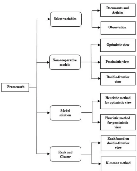
Each research is a systematic activity, in which either knowledge develops, or a situation is described and explained, or ultimately a particular problem is solved. Given that each research begins with a specific problem and purpose at hand, therefore, researches are of different types. Accordingly, this research is an applied research. The statistical population of this research includes the production, maintenance and distribution network of a factory (Nasiri Dairy factory), which is defined as an annual planning horizon in 24 periods. In this study, the methodology is designed in four steps. In the first step, the variables and data are collected based on the observation, interview and library studies. In the second step, a network data envelopment analysis (NDEA) approach is designed to measure the performance of DMUs based on the optimistic, pessimistic and double-frontier views. In the third step, a heuristic approach is designed, so as to resolve the optimistic and pessimistic models.Finally, in the fourth step, the decision-making units are ranked and classified by the k-means algorithm. In Fig. 1, the methodology is shown in four steps.
156
Fig 1. Steps of methodology
3-1- Model description
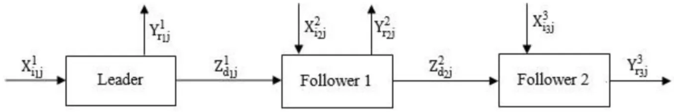
We consider a set of n homogeneous decision making units (DMUs) that are denote by DMUj
(j=1,..., n), and each DMUj (j=1,…,n) has three-stage, as shown in Fig. 2, where all the stages are
connected together in series. We denote, the inputs of the first stage by xi11j (i1=1,…,I1) and the
undesirable outputs of the first stage by yr1j 1 (r
1=1,…,R1). We denote, the intermediate measures
between first stage and second stage by zd11j (d1=1,…,D1) and between second stage and third stage
by zd22j (d2=1,…,D2). The additional inputs and outputs of the second stage are denoted by xi2j 2
(i2=1,…,I2) and yr2j 2 (r
2=1,…,R2), respectively. Finally, we denote, the additional inputs of the third
stage by xi33j (i
3=1,…,I3) and the outputs of the third stage by yr3j 3 (r
1=1,…,R3). We adopt vi1 1, v
i2 2 and
vi33 as the weights of the inputs to the first, second and third stages, respectively. Kao and Hwang
(2008) used the same weights for the intermediate measures. In accordance with this, we value the intermediate measures in this research, irrespective of its dual role (as an input in one stage or as an output in the next stage). We assume that the weights relative to the intermediate measures between stages 1 and 2 and similarly, weights in relevance with the intermediate measures between stages 2 and 3 are uniform. Therefore, we adopt w1d1 and wd22 as the weights of the intermediate measures
between stage 1, stage 2 and stage 3, respectively. The weights of the outputs for the first, second and third stages second stage are denoted by ur1
1, u r2 2 and u
r3
157
Fig 2. Structure of three-stage leader-follower system with additional inputs and undesirable outputs
Researchers are more inclined to utilize input-oriented models for efficiency analysis, mainly for three reasons. The first is that, demand reveals a growing trend, the estimation of which is an intricate matter. The second is that, managers have a better control on the inputs, rather than the outputs. The third is that, the model reflects the initial objectives of policy-makers, on the basis of being responsible in responding to the demands of the people. Furthermore, the units must reduce costs and or restrict the use of resources. Thereby, in this research, an input- oriented model is utilized. According to the opinions of managers, we shall describe and consider the first stage in the role of a “leader”, the second stage as the “first follower” and the third stage as the “second follower”. Thence, we demonstrate the optimistic and pessimistic efficiencies of the leader’s stage with θoL and φoL
respectively; the optimistic and pessimistic efficiencies of the second and third stages as θo1F, θo2F and
φo1F, φo2Frespectively; and the optimistic and pessimistic efficiencies of the second and third stages
together are shown as θo12F and φo12F respectively. In this section, which comprises of the proposed
approach of this paper, efforts have been made to insert the goals of the managers into the models. We designate the first stage as the “leader” and assume that the second and third stages together, are in the form of a “follower”. Under these conditions, the leader optimizes its efficiency so that the efficiency of the followers does not reduce from a certain level, or in actual fact, the leader maximizes its efficiency to forestall the eradication of the followers. Actually, the leader-follower characteristic is a non-cooperative game, which we hybrid with a cooperative approach in this section. In accordance with this, we describe the maximal efficiency of the leader stage from the optimistic viewpoint as hereunder:
θoL*=max {θoL| θo1F ≥ c1, θo2F ≥ c2, θjL ≤ 1, θj1F ≤ 1, θj2F ≤ 1, j=1,…,n } (1) All the variables in the model (1) are non-negative. Model (1) secures the maximal efficiency of the leader stage, on condition that, the efficiency of none of the stages is more than (1); and for DMU0 the follower stages (second and third stages) are not lower than the values of c1 and c2 respectively. The values of c1 and c2 are actually the minimal efficiency of the second and third stages which are numerals at intervals of (0 and 1) in accordance with the goals of managers. It should be noted that if the values of c1=c2 ε =are considered such, so that they are closer to (0), then the two constraints θo1F≥c1 and θo2F≥c2are simply redundant. So the model (1) is feasible. But there could be a
possibility that in reality, the goals of managers is not capable of being attained and the model turns into a superfluous one. Hence, we utilized the concept of ‘goal programming’ and the two assigned values 𝛼1and 𝛼2 are reduced (θo1F ≥ c1-𝛼1 θo2F ≥ c2-𝛼2) from the opinion of managers under
contemplation, so that by using model (2), conditions for securing the goal of managers is surveyed. Model (1) is a fractional model and by utilizing the Charnes-Cooper conversion (1962), as well as contemplating on the goal programming concept, as illustrated hereunder, it is converted into a linear model.
θoL*= max ∑dD11=1w1d1zd1o
1 -∑ u
r1 1 R1
r1=1 yr1o
1 -M(α
1+α2)
s.t. ∑I1 vi11 i1=1 xi1o
1 = 1
∑D1 wd11
d1=1 zd1j
1 -∑ u
r1 1 R1
r1=1 y1r1j-∑ vi1 1 I1
i1=1 xi1j
1 ≤ 0, j=1,…,n (2)
∑D2 wd22
d2=1 zd2j
2 +∑ u
r2 2 R2
r2=1 yr2j
2 -∑ v
i2 2 I2
i2=1 xi2j
2 -∑ w
d1 1 D1
d1=1 zd1j
1 ≤ 0,
j=1,…,n
158
∑ ur3 3 R3
r3=1 yr3j
3 -∑ v
i3 3 I3
i3=1 xi3j
3 -∑ w
d2 2 D2
d2=1 zd2j
2 ≤ 0, j=1,…,n
(c1- α1)∑dD11=1w1d1zd1o
1 + (c
1- α1)∑iI22=1v2i2xi2o
2 -∑ w
d2 2 D2
d2=1 zd2o
2 -∑ u
r2 2 R2
r2=1 yr2o 2 ≤ 0
(c2- α2)∑iI33=1v3i3xi3o
3 + (c
2- α2)∑dD22=1w2d2zd2o
2 -∑ u
r3 3 R3
r3=1 yr3o 3 ≤ 0
ur11,ur22,ur33≥ ε; r1=1,…,R1;r2=1,…,R2;r3=1,…,R3;
v1i1,vi22,vi33≥ ε;i1=1,…,I1; i2=1,…,I2; i3=1,…,I3; j=1,…,n. wd11,wd22≥ ε; d1=1,…,D1; d2=1,…,D2.
In the model (2) the optimum efficiency has been demonstrated with the symbol (*) and “M” denotes a large numeral, which factually is a penalty that causes the manager’s goal to be achievable. It should be mentioned that in the case where, α1=0,α2=0, the model (2) is feasible from the point of
the manager’s goal and if this is not the issue, we request the manager to reduce his goals ( ci) to the
measurement of αi to make the model possible. On the basis of the task of Wang et al. (2005), we
modify model (2), as hereunder to obtain the efficiency of the leader stage from the pessimistic view. Similar to our optimistic approach, we obtain the pessimistic efficiency of the leader stage, under conditions where the follower stages are at a distance from the inefficient frontier, i.e. φo2F ≥ c4- α4,
φo1F ≥ c
3- α3 in which case, c3,c4≥ 1.
φoL*= min ∑ w d1 1 D1
d1=1 zd1o 1
-∑ ur1 1 R1
r1=1 yr1o 1 + M(α
3+α4)
s.t. ∑I1 vi11 i1=1 xi1o
1 = 1
∑D1 wd11
d1=1 zd1j
1 -∑ u
r1 1 R1
r1=1 y1r1j-∑ vi1 1 I1
i1=1 xi1j
1 ≥ 0, j=1,…,n (3)
∑D2 wd22
d2=1 zd2j
2 +∑ u
r2 2 R2
r2=1 y2r2j-∑ vi2 2 I2
i2=1 xi2j
2 -∑ w
d1 1 D1
d1=1 zd1j
1 ≥ 0,
j=1,…,n
∑Rr33=1u3r3yr33j-∑ vi3 3 I3
i3=1 xi3j
3 -∑ w
d2 2 D2
d2=1 zd2j
2 ≥ 0, j=1,…,n
∑Dd22=1wd22zd22o+∑ ur22 R2
r2=1 yr2o 2 - (c
3- α3)∑ wd1 1 D1
d1=1 zd1o
1 - (c
3- α3)∑ vi2 2 I2
i2=1 xi2o 2 ≥ 0
∑Rr33=1u3r3yr33o- (c4- α4)∑iI33=1v3i3xi3o 3 - (c
4- α4)∑dD22=1w2d2zd2o 2 ≥ 0
ur11,ur22,ur33≥ ε; r1=1,…,R1;r2=1,…,R2;r3=1,…,R3;
v1i1,vi22,vi33≥ ε;i1=1,…,I1; i2=1,…,I2; i3=1,…,I3; j=1,…,n. wd11,wd22≥ ε; d1=1,…,D1; d2=1,…,D2.
Analogous to the optimistic approach of “M” that is a large numerical, which in this circumstance and with due attention to the type of objective function has been supplemented to the model in order to fulfill the manager’s goal. It should be observed that in the case where α1=0,α2=0, the model (3) is feasible in respect to the opinion of the manager or else we shall request the manager to reduce his goals of (ci) to the measurement of αi to make the model possible. Therefore, the maximal optimistic
efficiency of the leader stage θoL* and the minimal pessimistic efficiency of the leader stage φoL*is
brought to hand respectively, from models (2 and 3). To compute the efficiency of the followers we shall assume the second and third stages as one stage and obtain the efficiency of the follower stage. We hybrid the efficiencies of the second and third stages, being attentive to the fact that they are in series and define them as figures θo12F=θo1F .θo2F in accordance with the tasks of Kao and Hwang
(2008). Hence, the maximal efficiency together for the follower stages from the optimistic viewpoint is brought to hand as rendered hereunder:
159
θo12F*=max ∑ wd2
2 D2
d2=1 zd2o2 +∑R2r2=1ur22yr2o2 ∑I2 vi22
i2=1 xi2o2 +∑D1d1=1w1d1zd1o1
. ∑ ur3
3 R3 r3=1 yr3o3 ∑I3 v3i3
i3=1 xi3o3 +∑D2d2=1wd22 zd2o2
s.t. ∑ wd1
1 D1
d1=1 zd1j1 -∑R1r1=1ur11yr1j1 ∑I1 vi11
i1=1 x1i1j
≤1, j=1,…,n
∑ wd2
2 D2
d2=1 zd2j2 +∑R2r2=1ur22y2r2j ∑I2 vi22
i2=1 x2i2j+∑D1d1=1wd11 zd1j1
≤1, j=1,…,n (4)
∑ ur3
3 R3 r3=1 yr3j3 ∑I3 vi33
i3=1 xi3j3 +∑D2d2=1w2d2zd2j2
≤1, j=1,…,n
∑D1 wd11
d1=1 zd1o1 -∑R1r1=1ur11yr1o1 ∑I1 v1i1
i1=1 xi1o1
=θoL*
ur11,ur22,ur33≥ ε; r1=1,…,R1;r2=1,…,R2;r3=1,…,R3;
v1i1,vi22,vi33≥ ε;i1=1,…,I1; i2=1,…,I2; i3=1,…,I3; j=1,…,n. wd11,w2d2≥ ε; d1=1,…,D1; d2=1,…,D2.
The maximal and overall efficiency of the second and third stages is gained by model (4), on condition that, the efficiency of none of the stages equates to more than (1); and to the approach of Li et al. (2012), the efficiency of the leader’s stage should remain constant. On the founding’s of the tasks of Wang et al. (2005), we describe model (4) as given below, in order to attain the minimal efficiency of the overall follower stages from the pessimistic view.
φo12F*=min ∑ wd2 2 D2
d2=1 z2d2o+∑R2r2=1ur22yr2o2 ∑I2 vi22
i2=1 xi2o2 +∑D1d1=1w1d1zd1o1
. ∑ ur3
3 R3 r3=1 yr3o3 ∑I3 v3i3
i3=1 xi3o3 +∑D2d2=1wd22 zd2o2
s.t. ∑ wd1
1 D1
d1=1 zd1j1 -∑R1r1=1ur11yr1j1 ∑I1 vi11
i1=1 x1i1j
≥1, j=1,…,n
∑ wd2
2 D2
d2=1 zd2j2 +∑R2r2=1ur22y2r2j ∑I2 vi22
i2=1 x2i2j+∑D1d1=1wd11 zd1j1
≥1, j=1,…,n (5)
∑ ur3
3 R3 r3=1 yr3j3 ∑I3 vi33
i3=1 xi3j3 +∑D2d2=1w2d2zd2j2
≥1, j=1,…,n
∑D1 wd11
d1=1 zd1o1 -∑R1r1=1ur11yr1o1 ∑I1 v1i1
i1=1 xi1o1
=φoL*
ur11,ur22,ur33≥ ε; r1=1,…,R1;r2=1,…,R2;r3=1,…,R3;
v1i1,vi22,vi33≥ ε;i1=1,…,I1; i2=1,…,I2; i3=1,…,I3; j=1,…,n. wd11,w2d2≥ ε; d1=1,…,D1; d2=1,…,D2.
Models (4 and 5) are nonlinear and in the fourth section of this paper, an innovative approach in resolving it is utilized. In assuming that, the models are solved and given that the stages are in series
160
(figure 2), we define the total and maximal optimistic efficiency and the minimal and total pessimistic efficiency are respectively specified as below:
θooverall*= θoL* .θo12F*, φooverall*= φoL* .φo12F* (6)
Wang and Chin (2009) used an approach for ranking DMUs from both, the optimistic and pessimistic views. We then define the overall efficiency according to the double-frontier in formula (7) as below:
∅o*=√θooverall*.φooverall* (7)
3-2- Clustering
With the result of Formula (7), we can rank the DMUs. This ranking is based on the optimistic and pessimistic views. In the following, we use the k-means algorithm to cluster the DMUs into several groups. K-means clustering is a simple unsupervised learning algorithm that is used to solve clustering problems. It follows a simple procedure of classifying a given data set into a number of clusters, defined by the letter "k," which is fixed beforehand. The clusters are then positioned as points and all observations or data points are associated with the nearest cluster, computed, adjusted and then the process starts over using the new adjustments until a desired result is reached. The groups are determined in such a way that the similarity between the members of a group is high and the similarity between members of different groups is low. Given a set of observations (x1, x2, …,
xn), where each observation is a d-dimensional real vector, k-means clustering aims to partition the n
observations into k (≤ n) sets S = {s1, s2, …, sk} so as to minimize the within-cluster sum of squares
(WCSS) (i.e. variance). Formally, the objective is to find: arg min
s ∑ ∑ ‖x − μi‖
2 x∈si
k
i=1 =
arg min
s ∑ |si|Var si
k
i=1 where μi is the mean of points in si. In the K-Means algorithm, the k-member
is randomly selected from among the n members as cluster centers. Then the n-k remaining members are assigned to the nearest cluster. After assigning all members, the cluster centers are recalculated and the members are assigned to the clusters according to the new centers, and this continues until the centers of each cluster remain constant. In this paper, we use the k-means technique to cluster the results of the described models (cluster based on the result of the formula (6)) and these results are shown in the case study section. In order to select the best cluster, based on expert opinions and previous studies, a suggested range for the number of clusters was initially identified. In accordance with the opinions of managers, we suggest to cluster the DMUs into three groups (k=3) with similar characteristics.
4- Heuristic approach to solve nonlinear models
In this section we will use a solution to gain the efficiency of the followers. Due to the presence of additional inputs and outputs in the first, second and third stages, models (4 and 5) are nonlinear. To solve these models we use a heuristic approach as hereunder:
4-1- A heuristic method from optimistic view
We are aware that the objective function of model (4) is the multiplicative efficiency of the two-stages, i.e. θo12F*=maxθ1Fo .θo2F. We take θo1F as a variable in the objective function which modifies
between the [0, θo1F-max ] interval. We describe θo1F as given below, so that we are able to move it
between intervals.
θo1F = θo1F-max - k1∆ε, k1=0,1,…,[θo 1F- max
∆ε ]+1 (8)
We take ∆ε as a step size and consider it an extremely small amount and describe θo1F-max as the
maximum efficiency of the first follower stage and its value is capable of being computed by the model below.
161
Model (9) secures the maximum efficiency of the first follower stage, under conditions where the efficiency of all the stages is less than (1). In actual fact, this model irrespective, of the leader-follower correlations, attributes the highest efficiency to the second stage. This model is a fractional model and by utilizing the Charnes-Cooper conversion (1962), as illustrated hereunder, it is converted into a linear model.
θo1F-max= max ∑ wd2 2 D2
d2=1 zd2o
2 +∑ u
r2 2 R2
r2=1 yr22o
s.t. ∑Ii11=1v2i2xi2o
2 +∑ w
d1 1 D1
d1=1 zd1o
1 = 1
∑Dd1 wd11
1=1 zd1j
1 -∑ u
r1 1 R1
r1=1 yr1j
1 -∑ v
i1 1 I1
i1=1 xi1j
1 ≤ 0, j=1,…,n (10)
∑D2 w2d2
d2=1 zd2j
2 +∑ u
r2 2 R2
r2=1 yr2j
2 -∑ v
i2 2 I2
i2=1 xi2j
2 -∑ w
d1 1 D1
d1=1 zd1j
1 ≤ 0,
j=1,…,n
∑ ur33 R3
r3=1 yr3j
3 -∑ v
i3 3 I3
i3=1 xi3j
3 -∑ w
d2 2 D2
d2=1 zd2j
2 ≤ 0, j=1,…,n
ur11,ur22,ur33≥ ε; r1=1,…,R1;r2=1,…,R2;r3=1,…,R3;
vi11,vi22,vi33≥ ε;i1=1,…,I1; i2=1,…,I2; i3=1,…,I3; j=1,…,n. w1d1,wd22≥ ε; d1=1,…,D1; d2=1,…,D2.
In determining the value of θo1F-max by model (10), we convert model (4) into the following model.
θo12F*=max {θo1F.θo2F| θjL ≤ 1, θj1F ≤ 1, θj2F ≤ 1, θoL=θoL*,θo1F= Oo 2 Io2 , θo
1F ∈[0, θ o
1F-max ], j=1,…,n }
(11)
In the model (11) we considered θo1F in the objective function as a variable and the constraint which
specified this variable, together with its interval of modification was added to the model. In model (11), we have demonstrated the efficiency of the second stage or θo1F briefly, in a form of output to an
input. The model (11) is a fractional one and by utilizing the Charnes-Cooper conversion (1962), as illustrated hereunder, it is converted into a linear model.
θo12F*= max θo1F .∑R3 ur33 r3=1 yr3o
3
s.t. ∑I3 v3i3 i3=1 xi3o
3 +∑ w
d2 2 D2
d2=1 zd2o
2 = 1
∑D1 wd11
d1=1 zd1j
1 -∑ u
r1 1 R1
r1=1 yr1j
1 -∑ v
i1 1 I1
i1=1 xi1j
1 ≤ 0, j=1,…,n (12)
∑D2 wd22
d2=1 zd2j
2 +∑ u
r2 2 R2
r2=1 yr2j
2 -∑ v
i2 2 I2
i2=1 xi2j
2 -∑ w
d1 1 D1
d1=1 zd1j
1 ≤ 0,
j=1,…,n
∑Rr33=1ur33yr3j
3 -∑ v
i3 3 I3
i3=1 xi3j
3 -∑ w
d2 2 D2
d2=1 zd2j
2 ≤ 0, j=1,…,n
∑Dd11=1w1d1zd1o
1 -∑ u
r1 1 R1
r1=1 yr1o
1 -θ
o
L*∑ v
i1 1 I1
i1=1 xi1o 1 = 0
∑Dd2 wd22
2=1 zd2o
2 +∑ u
r2 2 R2
r2=1 yr2o
2 -θ
o
1F*(∑ v
i2 2 I2
i2=1 xi2o
2 +∑ w
d1 1 D1
d1=1 zd1o
1 )=0
θo1F ∈[0, θo1F-max ]
ur11,ur22,ur33≥ ε; r1=1,…,R1;r2=1,…,R2;r3=1,…,R3;
v1i1,vi22,vi33≥ ε;i1=1,…,I1; i2=1,…,I2; i3=1,…,I3; j=1,…,n. wd11,w2d2≥ ε; d1=1,…,D1; d2=1,…,D2.
162
In model (12) and by utilizing formula (8), we increase the value of k1 from (0) to its higher level, in order to solve the new model each time with θo1F . We solve the returns of the entire conditions of the
k1 model and the responses of the model is assigned as θo12F(k1). By comparing all the values of
θo12F(k
1), we define θo12F* as the maximal efficiency of the total sum of the follower stages from the
optimistic view. It should be noted that, we have tested our proposed approach under two conditions and each time have considered a stage as a variable. Given that the efficiency of a stage is somewhat unique, thereby, the results of these two methods have come to hand with an extremely good approximation and in order to explain our approach, we have denoted one of these two conditions above.
3-2- A heuristic method from pessimistic view
We know that the objective function of model (5) is the multiplicative efficiency of two stages,
i.e. φo12F*=min φo1F. φo2F. Similar to our optimistic view, we take φo1F as a variable in the objective
function that modifies between the [φo1F-min ,M] interval. We describe φ o
1F as rendered below so that
we can move it within the interval. φo1F = φ
o
1F-min + k
1∆ε, k1=0,1,…,[
M-φo1F- min
∆ε ]+1 (13)
We consider “M” to be a large amount and alike the optimistic approach, ∆ε as a step size and an extremely small amount. φo1F-min is described as the minimum efficiency of the first follower stage
and its sum can be computed by the following formula. φo1F-min=min {φ
o 1F| φ
j L ≥ 1, φ
j
1F ≥ 1, φ j
2F ≥1, j=1,…,n } (14)
Model (14), secures the minimum efficiency of the first follower stage, on condition that the efficiency of all the stages is more than (1). In fact, this model, regardless to the leader-follower correlation, attributes the least amount of efficiency to the second stage. This model is a fractional model and by employing the Charnes-Cooper conversion (1962), it is converted into a linear model as given hereunder:
φo1F-min= min ∑ w
d2 2 D2
d2=1 zd2o
2 +∑ u
r2 2 R2
r2=1 yr2o
2
s.t. ∑I2 vi22
i2=1 xi2o
2 +∑ w
d1 1 D1
d1=1 zd1o
1 = 1
∑D1 wd11
d1=1 zd1j
1 -∑ u
r1 1 R1
r1=1 yr11j-∑ vi1 1 I1
i1=1 xi1j
1 ≥ 0, j=1,…,n (15)
∑D2 w2d2
d2=1 zd2j
2 +∑ u
r2 2 R2
r2=1 yr2j
2 -∑ v
i2 2 I2
i2=1 xi2j
2 -∑ w
d1 1 D1
d1=1 zd1j
1 ≥ 0,
j=1,…,n
∑ ur3 3 R3
r3=1 yr3j
3 -∑ v
i3 3 I3
i3=1 xi3j
3 -∑ w
d2 2 D2
d2=1 zd2j
2 ≥ 0, j=1,…,n
ur11,ur22,ur33≥ ε; r1=1,…,R1;r2=1,…,R2;r3=1,…,R3;
vi11,vi22,vi33≥ ε;i1=1,…,I1; i2=1,…,I2; i3=1,…,I3; j=1,…,n. wd11,wd22≥ ε; d1=1,…,D1; d2=1,…,D2.
In specifying the value of
φ
o1F-min by model (15), model (5) is modified and converted to themodel below: φo12F*=min {φ o 1F.φ
o 2F| φ
j L ≥ 1, φ
j
1F ≥ 1, φ j
2F ≥ 1, φ o L=φ
o L*, φ
o 1F= Oo2
Io2 , φo 1F ∈[φ
o
1F-min ,M], j=1,…,n } (16)
163
It should be brought to attention that, in the model (16), we take φo1F in the objective function as a
variable and alike the optimistic approach, constraints which specify this variable, along with its interval of modification is supplemented to the model. The model (16) is a fractional model and by using the Charnes-Cooper conversion (1962), it is converted into a linear model as given hereunder: φo12F*= min φ
o
1F .∑ u
r3 3 R3
r3=1 yr3o
3
s.t. ∑I3 v3i3 i3=1 xi3o
3 +∑ w
d2 2 D2
d2=1 zd2o
2 = 1
∑D1 wd11
d1=1 zd1j
1 -∑ u
r1 1 R1
r1=1 y1r1j-∑ vi1 1 I1
i1=1 xi1j
1 ≥ 0, j=1,…,n (17)
∑D2 wd22
d2=1 zd2j
2 +∑ u
r2 2 R2
r2=1 yr2j
2 -∑ v
i2 2 I2
i2=1 xi2j
2 -∑ w
d1 1 D1
d1=1 zd1j
1 ≥ 0,
j=1,…,n
∑Rr33=1u3r3yr33j-∑ vi3 3 I3
i3=1 xi3j
3 -∑ w
d2 2 D2
d2=1 zd2j
2 ≥ 0, j=1,…,n
∑Dd11=1w1d1zd11o-∑ ur11 R1
r1=1 yr1o
1 -φ
o
L*∑ v
i1 1 I1
i1=1 xi1o 1 = 0
∑D2 wd22
d2=1 zd2o
2 +∑ u
r2 2 R2
r2=1 yr22o-φo1F*(∑ vi2 2 I2
i2=1 xi2o
2 +∑ w
d1 1 D1
d1=1 zd1o
1 )=0
φo1F ∈[φo1F-min ,M]
ur11,ur22,ur33≥ ε; r1=1,…,R1;r2=1,…,R2;r3=1,…,R3;
v1i1,v2i2,vi33≥ ε;i1=1,…,I1; i2=1,…,I2; i3=1,…,I3; j=1,…,n. wd11,wd22≥ ε; d1=1,…,D1; d2=1,…,D2.
In model (17) and by employing formula (13), we increment the value of k1 to its utmost level, in order to solve the model each time with the new φo1F . we resolve the entire the returns of the
conditions of the k1 model and the responses of the model is denoted by φo12F(k1) . By comparing all the values of φo12F(k1), we define φo12F*as the minimal efficiency of the total sum of the follower
stages from the pessimistic view. It should be noted that, similar to the optimistic approach, we have tested our proposed approach under two conditions and each time have considered a stage as a variable; with due attention to the fact that, the efficiency of a stage is somewhat unique, thereby, the results of these two methods have come to hand with an extremely good approximation and in order to explicate our approach, we have represented one of these two conditions above.
5- Case Study description
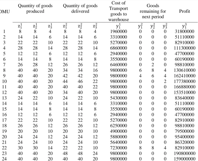
In the authentic world, a factory produces three products. This factory has a production area, a warehouse area and a delivery point. We consider each one of these as a stage. The production area plays the role of the “leader” and the other two, the role of “followers”. We have contemplated on this factory for within a length of 24 time periods and as a dynamic network. In this network, a number of outputs during a time period of t in the second stage are converted to a number of inputs in the second stage during a time period of t+1. We assume each time period to be a DMU. Hence, the inputs and outputs of each DMU are according to the following. We assign the production costs of the three products produced as an input of the first stage and denote it as (x11,x21,x31). The transport costs for
produce from the first to the second stage is described as an undesirable output of the first stage, which we show as y11. The intermediary produce between the first and second stages, is the quantityof
produce of each commodity, which is demonstrated as (z11, z
12, z13). The additional outputs for the
second stage are respectively, the cost of reserving storage location x12 cost of holding goods x 2 2and
164
define the output of the second stage as the quantity of the remaining goods in the warehouse for the subsequent period of time, and represent it with (y12,y22,y32). The intermediary products between the
second and third stages are the quantities of delivery of each commodity, which is demonstrated by
(z14, z15, z16). We describe the additional inputs of the third stage as the transport costs of goods to the third stage and this is illustrated as x13. Finally, the output of the third stage is the profit from the sale
of goods, which is indicated by y13. In continuation, we illustrate the input values for the 24 time
periods in table 1 and the mean values and outputs in table 2.
Table 1. The inputs of the factory for 24 period in 2016
DMU Production cost
Cost of reserving
storage location
Cost of holding goods
Goods remaining from
last period
Cost of Transport
goods to delivery points
x11 x
2
1 x
3
1 x
1
2 x
2
2 x
3
2 x
42 x52 x13
1 29120000 36160000 51520000 1700000 1430000 0 0 0 3680000
2 50960000 63280000 77280000 1700000 1430000 0 0 0 6235000
3 80080000 99440000 128800000 1700000 1430000 0 0 0 9915000
4 101920000 126560000 180320000 1700000 1430000 0 0 0 12880000
5 43680000 54240000 77280000 1700000 1430000 0 0 0 5520000
6 50960000 63280000 103040000 1700000 1430000 0 0 0 6645000
7 94640000 126560000 154560000 1700000 1670000 0 0 0 11755000
8 145600000 180800000 257600000 1700000 3620000 0 2 0 15435000
9 145600000 180800000 257600000 1700000 3170000 6 8 4 19115000
10 145600000 180800000 257600000 1700000 1730000 4 6 4 20555000
11 145600000 180800000 257600000 1700000 1430000 0 0 2 19220000
12 145600000 180800000 257600000 1700000 1430000 0 0 0 16815000
13 87360000 99440000 128800000 1700000 1430000 0 0 0 10290000
14 50960000 63280000 77280000 1700000 1430000 0 0 0 6235000
15 50960000 63280000 103040000 1700000 1430000 0 0 0 6645000
16 43680000 54240000 77280000 1700000 1430000 0 0 0 5520000
17 80080000 99440000 128800000 1700000 1430000 0 0 0 9915000
18 94640000 117520000 154560000 1700000 1430000 0 0 0 11755000
19 72800000 90400000 128800000 1700000 1430000 0 0 0 9200000
20 87360000 108480000 154560000 1700000 1430000 0 0 0 11040000
21 87360000 108480000 128800000 1700000 1430000 0 0 0 10630000
22 109200000 135600000 180320000 1700000 3830000 0 0 0 9915000
23 145600000 180800000 257600000 1700000 1430000 8 8 4 22080000
24 145600000 180800000 257600000 1700000 1430000 0 0 0 18400000
In the table 1, the values of (0), for each period indicate that, the goods have not remained in the warehouse since the previous period (columns 7 to 9). The following table 2, also shows values with (0), which illustrate that the goods for the subsequent period have not remained in the warehouse (columns 9 to 11).
165
Table 2. The outputs and the intermediate measures of the factory for 24 periods in 2016
Profit Goods remaining for next period Cost of Transport goods to warehouse Quantity of goods
delivered Quantity of goods
produced DMU
y13
y32
y22
y12
y11
z32
z22
z12
z31
z21
z11
31800000 0 0 0 1960000 4 8 8 4 8 8 1 51110000 0 0 0 3310000 6 14 14 6 14 14 2 82910000 0 0 0 5270000 10 22 22 10 22 22 3 111300000 0 0 0 6860000 14 28 28 14 28 28 4 47700000 0 0 0 2940000 6 12 12 6 12 12 5 60190000 0 0 0 3550000 8 14 14 8 14 14 6 98810000 0 2 0 6460000 12 26 26 12 28 26 7 130610000 4 8 6 9800000 16 34 34 20 40 40 8 162410000 4 6 4 9800000 20 42 42 20 40 40 9 177380000 2 0 0 9800000 22 46 44 20 40 40 10 166880000 0 0 0 9800000 22 40 40 20 40 40 11 153510000 0 0 0 9800000 20 40 34 20 40 40 12 83640000 0 0 0 5430000 10 22 24 10 22 24 13 51110000 0 0 0 3310000 6 14 14 6 14 14 14 60190000 0 0 0 3550000 8 14 14 8 14 14 15 47700000 0 0 0 2940000 6 12 12 6 12 12 16 82910000 0 0 0 5270000 10 22 22 10 22 22 17 98810000 0 0 0 6250000 12 26 26 12 26 26 18 79500000 0 0 0 4900000 10 20 20 10 20 20 19 95400000 0 0 0 5880000 12 24 24 12 24 24 20 86320000 0 0 0 5640000 10 24 24 10 24 24 21 82910000 4 8 8 7230000 10 22 22 14 30 30 22 190800000 0 0 0 9800000 24 48 48 20 40 40 23 159000000 0 0 0 9800000 20 40 40 20 40 40 24
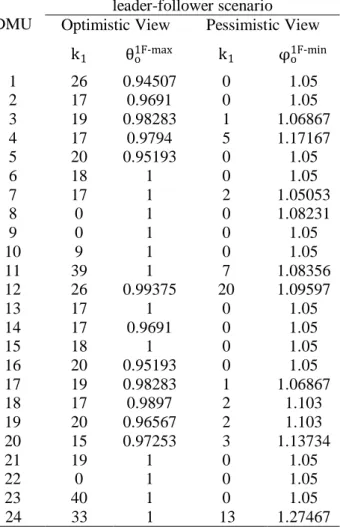
In continuation, we secure the efficiency of the factory from a leader-follower scenario. For this purpose, c1= c2=0.6 and c3= c4=1.05 are considered as goals of managers. The values of
(αi=0, i=1,2,3,4) have come to hand from models (2 and 3) and show that the goals of the managers
has been attained. In the leader-follower scenario, on the basis of the opinions of managers, ∆ε=0.01
and M=3 have been considered. Similarly, the value for 𝜀 in all the models has been considered as 0.05 by the managers. We have executed the heuristic method expressed in the section (4). The values achieved for 𝑘1 together with the maximal optimistic efficiency and the minimal pessimistic
166
Table 3. Results of the maximum and minimum efficiencies of the first stage and k values
leader-follower scenario
DMU Optimistic View Pessimistic View
φo1F-min
k1
θo1F-max
k1
1.05 0
0.94507 26
1
1.05 0
0.9691 17
2
1.06867 1
0.98283 19
3
1.17167 5
0.9794 17
4
1.05 0
0.95193 20
5
1.05 0
1 18
6
1.05053 2
1 17
7
1.08231 0
1 0
8
1.05 0
1 0
9
1.05 0
1 9
10
1.08356 7
1 39
11
1.09597 20
0.99375 26
12
1.05 0
1 17
13
1.05 0
0.9691 17
14
1.05 0
1 18
15
1.05 0
0.95193 20
16
1.06867 1
0.98283 19
17
1.103 2
0.9897 17
18
1.103 2
0.96567 20
19
1.13734 3
0.97253 15
20
1.05 0
1 19
21
1.05 0
1 0
22
1.05 0
1 40
23
1.27467 13
1 33
24
In studying the values of k, we were aware that, in this case study, that the pessimistic efficiency of the first follower, in most of the cases, is optimized, when the values of k are low (column 4). This signifies that, the optimal efficiency value of the second stage or the first follower are proximate to their minimum values (columns 5), whereas, in the case of the optimistic efficiency value of the second stage, are far from their maximum value, in most circumstances (columns 3). Table 4 gives the overall efficiency and the efficiencies of stages based on the optimistic and pessimistic views.
167
Table 4. Results based on the optimistic and pessimistic views
Pessimistic View Optimistic View
DMU
φo2F*
φo1F*
φoL*
φooverall*
θo2F* θo1F*
θoL* θooverall*
1.05 1.05 1 1.1025 0.72563 0.68507 1 0.49711 1 1.05 1.05 1 1.1025 0.61713 0.7991 1 0.49315 2 1.05 1.07867 1 1.1326 0.63265 0.79283 1 0.50159 3 1.05 1.22167 1 1.28275 0.60449 0.8094 1 0.48928 4 1.05 1.05 1 1.1025 0.67144 0.75193 1 0.50488 5 1.05 1.05 1 1.1025 0.68081 0.82 1 0.55827 6 1.05 1.07053 1 1.12406 0.60559 0.83 1 0.50264 7 1.05 1.08231 1 1.13643 0.72931 1 1 0.72931 8 1.05 1.05 1 1.1025 0.68483 1 1 0.68483 9 1.05 1.05 1 1.1025 0.67609 0.91 1 0.61525 10 1.0558 1.15356 1 1.21794 0.60542 0.61 1 0.36931 11 1.05 1.29597 1 1.36077 0.60002 0.73375 1 0.44027 12 1.05 1.05 1 1.1025 0.60109 0.83 1 0.49891 13 1.05 1.05 1 1.1025 0.61713 0.7991 1 0.49315 14 1.05 1.05 1 1.1025 0.68081 0.82 1 0.55827 15 1.05 1.05 1 1.1025 0.67144 0.75193 1 0.50488 16 1.05 1.07867 1 1.1326 0.63265 0.79283 1 0.50159 17 1.05 1.123 1 1.17915 0.60045 0.8197 1 0.49219 18 1.05 1.123 1 1.17915 0.66846 0.76567 1 0.51182 19 1.05 1.16734 1 1.22571 0.62146 0.82253 1 0.51117 20 1.05 1.05 1 1.1025 0.60153 0.81 1 0.48724 21 1.05 1.05 1 1.1025 0.79076 1 1 0.79076 22 1.05 1.05 1 1.1025 0.6 0.6 1 0.36 23 1.05 1.40467 1 1.4749 0.60471 0.67 1 0.40516 24
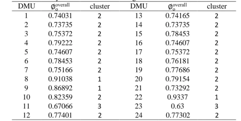
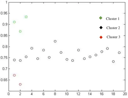
From the second column of table 4, we note that the efficiency scores of period 22 is the highest and the efficiency scores of period 23 is the lowest, from the optimistic view. The sixth column of Table 4, show that the efficiency scores of period 24 is the highest and the efficiency scores of periods 1,2,5,6,9,10,13,14,15,16,21,22 and 23 is the lowest, from the pessimistic view. By comparing the results, we observe that the difference in optimistic and pessimistic views in some cases, for example, by looking at the second column of table 4, we find that, the efficiency scores of period 10 is higher than period 11 )0.61525 > 0.36931) from the optimistic view. But, from the sixth column of Table 4, it can be noted that, period 11 is higher than period 10 (1.1025 > 1.21794) from pessimistic view. Therefore, for the final ranking of DMUs, we use the double-frontier or the optimistic and pessimistic views that we have explained in the section (3) by formula (7). Table 5 gives the overall efficiency and clustering results based on the double-frontier view.
Table 5. The efficiency evaluation and clustering results based on the double-frontier view cluster
∅ooverall
DMU cluster
∅ooverall
DMU 2 0.74165 13 2 0.74031 1 2 0.73735 14 2 0.73735 2 2 0.78453 15 2 0.75372 3 2 0.74607 16 2 0.79222 4 2 0.75372 17 2 0.74607 5 2 0.76181 18 2 0.78453 6 2 0.77686 19 2 0.75166 7 2 0.79154 20 1 0.91038 8 2 0.73292 21 1 0.86892 9 1 0.9337 22 2 0.82359 10 3 0.63 23 3 0.67066 11 2 0.77302 24 2 0.77401 12