Order Statistics Bayesian–Mining Agent Modelling for Automated
Negotiation
Samir Abdel Rahman, Reem Bahgat and George M. Farag Computer Science Department,
Faculty of Computers and Information, Cairo University, Egypt
E-mail: {s.abdelrahman, r.bahgat}@fci-cu.edu.eg, [email protected]
Keywords:bayesian mining, order statistics, automated negotiation, multi-issue, multi-session, opponent modelling
Received:May 27, 2010
The availability of qualitative knowledge has been recently used to simulate human negotiations accurately. During real-life negotiation sessions, people accumulate their knowledge to opt for most adequate bids by which both negotiating parties reach a win-win agreement. Unfortunately, existing research mainly concentrates on few negotiation bids. This paper proposes order statistics Bayesian-mining agent approach to automate bilateral multi-issue multi-session win-win negotiation problems. The proposed agent applies a real-life social bid ranking based on historical bids of all previous negotiation sessions to dynamically update all issues’ weights and preferences. Moreover, it uses our proposed deterministic Trade-Off counter offer method, rather than the existing haphazard estimation method, to estimate precisely the next bid. Experiments are conducted on 3-issue, 5-issue, 6-issue and 10-issue having 27, 3169, 3122 and 13219200 bids respectively. The selected evaluation analysis methods are mainly Pareto optimality, utility, cost and step-wise measurements. Compared with existing agent sorts, such as ABMP, Trade-Off, Bayesian and Mining agents, the proposed agent approach is proved that it is more efficient, effective, scalable and sensitive (adaptable to the opponent steps). Also, it works better to maximize its utilities and to minimize the negotiation costs (the number of rounds).
Povzetek: Opisana je agentna metoda pogajanj, ki se odloča na osnovi Bayesovske statistike.
1
Introduction
The paper aims to automate bilateral issue multi-session win-win human negotiation. Negotiation is the process in which two or more parties, having conflicts in their interests, can mutually reach a beneficial agreement on the related set of issues by exchanging some bids. In any bilateral negotiation [20], there are only two parties who exchange their bids using some negotiation protocols. In multi-issue negotiations [20], each bid has many issues such that each issue consists of several discrete items. The negotiator goal is to adjust all issues’ preferences to maximize his bid utility. The essential assumption of win-win multi-issue bilateral negotiation is that the two negotiators are rational and they are eager to find a solution of bid utilities that is acceptable to both parties [19]. So, each party has to know the preferences of its opponent to reach an agreement. In reality, the negotiators are hardly willing to disclose their private preferences. Consequently, both parties have incomplete information about each other and so may hardly reach an optimal deal. A typical real-life negotiation may need more than one session to reach a successful deal such that each party commences the new session having some gained knowledge about his opponent from previous sessions, where a session is defined as the time duration in which the negotiators decide to communicate with each other to reach a satisfied agreement, if any.
Automated negotiation recently has become a disputed solution to compensate the human disability to do complicated negotiation calculations accurately.
Automated negotiation applications range from simple auctions, in which agents merely have to bid truthfully [29], to complex strategic models, in which agents argue for positions and aim to persuade their opponents of the particular course of action [24].
Some multi-agent research [2, 9, 12] presented strategies to automate multi-issue negotiation. Such research was usually motivated with the high complexity of multi-issue negotiation calculations executed with the lack of available knowledge about the opponent. Recently, some research [7, 12] investigated the use of available knowledge about the environment’s bids, issues, or opponent preferences while negotiation sessions move forward. However, they either concentrated on cases having one issue or they depended on few bids from previous/current single session negotiation. Moreover, their assumptions of issue ranking and the data distribution are theoretical rather than experimental; real-life applications are complex in which the agreement is met after successive negotiations having massive hidden information about the environment’s preferences and issues that could be mined, i.e. extracted and accumulated, while the negotiation sessions ensue.
proposed model gradually learns how to reduce the number of session rounds and to maximize the expected utility upon the ratio of accepted bids. To do that, the model weighs the bids, similar to the human ranking, by which the first bid from each session is the most significant bid and the current session is the most vital session. The model then utilizes order statistics, non-parametric, Bayesian learning to model the opponent preferences and profiles which deals with any unknown data distribution.
Second, a proposed trade-off counter-offer method is used to estimate the next bid more precisely. This is done by replacing existing randomness trade-off method with a proposed partial derivative utility function.
Our experiments are set up against some well-known existing agent approaches using 3-issue, 5-issue, 6-issue and 10-issue applications. We use some evaluation criteria, namely Pareto optimality, utility, cost (number of rounds), step-wise (sensitivity analysis and class studies), and confidence interval calculations. It is experimentally proved that any agent following our proposed model is efficient, effective and sensitive to the opponent steps. Also, the proposed agent scalability is verified as the agent guarantees these features on 10-issue applications.
In comparison with current negotiation approaches, the contributions of the proposed non-parametric Bayesian-mining approach are as follows:
1-It works with any negotiation data distribution; all current approaches assume normal distribution of data, which is not necessarily true.
2-The agent outcomes are more effective and sensitive as the agent can benefit from the historical data of all previous negotiation sessions.
3-When our agent is involved in the negotiation, better agreement is reached fast.
4-When our agent is involved in the negotiation, both negotiators tend to maximize their utilities.
5- Our approach is scalable for large data set, while authors of the other approaches state that they have to adapt their models, if possible, to make them acquire such a feature.
The remainder of this paper is organized as follows. The next section discusses other negotiation approaches. Section 3 outlines the evaluation methods stated in the literature. Section 4 presents the overall proposed approach with its assumptions and parameters. Section 5 demonstrates the proposed Bayesian-mining approach. Section 6 presents the proposed counter-offer enhancement. Section 7 shows the experimental results. The paper is concluded with Section 8.
2
Related work
ABMP strategy [15, 16] takes the agent’s own utility space in which the next bid utility has less value than the previous one. Unfortunately, the strategy does not use any domain or opponent knowledge. Also it does not search through the negotiation outcome space for results that are mutually beneficial for both parties. Therefore, this strategy is inefficient in complex negotiation
domains although it is shown that it outperforms humans in small domains [1].
Trade-off strategy [9] is based on similarity and iso-curve criteria. In this strategy, the agent tries to find a bid similar to his previously proposed one and to be simultaneously suitable for his opponent. However the random nature of its search impacts on its efficiency. Another disadvantage is its difficulty to determine the bid suitability for the opponent’s utility without having any knowledge about his preferences. So, it always needs a complement strategy to detect the opponent preferences.
Bazaar model [33] is a learning approach for sequential decision making in a single session single issue (the price) negotiation. It works by generating random numbers of upper and lower limits for the agent’s reservation price to ensure the existence of agreement zone. However, the negotiation model is dedicated only to the price issue which is already known earlier to both agents.
A Bayesian Markov chain model [21] was presented to learn the opponent preferences in single issue negotiation. Its major defect is that it does not have a state-memory to save all negotiation movements since it depends only on the negotiation current state to predict the future bids. Moreover, it works only on a single issue.
Kernel Density Estimator model [7], based on [9], provided a kernel estimation method that depends on the difference between two bids to predict the issue weight. Therefore, the estimator doesn’t use its whole available negotiation history to define its kernel. Moreover, it does not provide a learning method for estimating the issue weights, hence, it may be used effectively only with single issue negotiations.
A Bayesian learning modelling [12] was presented to learn an opponent model, i.e. the issue preferences and priorities of the opponent. Unfortunately, the model uses single session only to know the opponent preferences. In most cases, the session has few bids to learn and thus the gained knowledge is often imperfect. Also, it enumerates all possible issue-weight ranks to form the weighted issue hypothesis space which makes the space considerably huge. Moreover, as most strategies do, it assumingly considers the negotiation data to follow the normal distribution which contradicts with real human negotiations.
buyers.
As shown above, current automated negotiation strategies don’t exploit all historical bids to enhance the negotiation outcomes. Moreover, they follow some theoretical assumptions which make the negotiation relatively far from reality.
We compare our work with the above mentioned approaches to prove our approach’s efficiency, effectiveness, sensitivity to the opponent steps, and scalability. Fortunately, some research, such as [12, 23], tried to prove the scalability of their approaches. They report that it is not easy for any model to sustain high dimensional specifications. The authors of Bayesian Learning model [12] show that they modify their model to make it scalable for 10-issue applications and when compared with the Trade-Off agent, both performances were similar to each other as the agents stay close to the Pareto frontier. In [23], a system of artificial adaptive agents (AAAs), is created and tested for 10-issue against the human agents to evaluate their performance. The authors find that in high dimensions, such as 10-issue, it is very complicated to make a suitable comparison of the behavior and the performance between AAA and human agents since neither the two agents may outperform each other.
Before presenting the proposed framework strategy (Sections 4, 5 and 6), it is also worth exploring the real-life win-win bilateral game strategy. Three cases are possible. The first case is when both players are unprofessional or not able to accumulate knowledge about each other, then the game outcomes are weak. The second case is when one of them is skilful to gain experience from his opponent tactics, then he outperforms his opponent even if he commences the game weakly. Moreover, the game outcomes are relatively high. The last case is when both players are professional, i.e. they can benefit or learn knowledge about the tactics of each other, which may positively affect both of them on the general results of the game. If such game is negotiation, then people benefit from the past/current sessions to achieve the best, even if they have little initial data about their opponents. People always give the highest priority to the first bid in each session and lower priorities to successive bids. Also, they give weights to previous sessions and their bids but the weights reduce as the sessions are further away from the current session.
3
Evaluation methods
Most existing automated negotiation approaches consider mainly Pareto optimality [6, 8, 27], utility [17, 31], cost (number of rounds) [33] and step-wise (sensitivity analysis and class studies) [13] criteria as their evaluation methods. They consider the negotiation of an agent efficient if its outcomes have rapidly reached the Pareto Frontier with the maximum utilization and the minimum number of rounds. Also, they prove the agent effectiveness using Pareto optimality and sensitivity analysis. People, then, apply sensitivity analysis and class studies to test the negotiator adaptability to the
opponent preferences. We use all these methods to evaluate our proposed model.
3.1
Pareto Optimality
This method is to measure the distance of the negotiation outcome to the Pareto Frontier. A deal is Pareto optimal (or Pareto efficient), if it is not dominated by any other deal. In other words, a deal is Pareto optimal if it is the best agreement among all negotiation agents. When the deal is Pareto optimal, the negotiation should end with such an agreement [17, 31].
3.2
Cost Analysis
The cost of a negotiation process is measured by the number of proposals (rounds) exchanged before reaching an agreement [33]. The agent is efficient if it does fewer rounds to reach optimum agreement with its opponent.
3.3
Utility Analysis
An automated negotiation strategy should guarantee its agent to reach the maximum utilities when the agreement deal is committed. An efficient negotiation strategy models its agent such that it swiftly increases the outcomes while the negotiation sessions advance.
3.4
Sensitivity Analysis
In the sensitivity analysis [13], not only the study of negotiation outcomes is essential, but also the investigation of the agent faults which are realized throughout the negotiation activities. Another useful sensitivity analysis of the opponent preferences is to dynamically find out the negotiation characterizations. It can be defined by comparing the percentage (Equation 1) of fortunate, nice and concession steps that increases the opponent’s utility to the percentage of selfish, unfortunate and silent steps that decreases it. Spontaneously, an agent which only achieves steps increasing its opponent utility can be said to be sensitive to its opponent requirements.
A single negotiation step between an agent current bid and the previous one for that agent which is written as [13] based on utilities as follows:
s Ua
b Ua
ba
(1)
For a step
s
b
a
b
a
,a
S
,
O
, for the AgentS
and its OpponentO
, to denote the utility difference of two bids b and b’ in the utility space of agent A. From the point of view of the agent S, the negotiation step sis classified as [13]: Fortunate Step, denoted by (S+, O+), iff:
∆S(s)>0, and ∆O(s)>0.
Selfish Step, denoted by (S+, O≤), iff:
∆S(s)>0, and ∆O(s)≤0.
Concession Step, denoted by (S-, O≥), iff:
∆S(s)<0, and ∆O(s)≥0.
Unfortunate Step, denoted by (S≤, O-), iff:
Nice Step, denoted by (S=, O+), iff:
∆S(s)=0, and ∆O(s)>0.
Silent Step, denoted by (S=, O=), iff:
∆S(s)=0, and ∆O(s)=0.
The measure for sensitivity of the agent
A
(Equation 2) to its opponent’s preferences is defined for a
given trace
t
[13] which includes all session bids for bothagents.
)
(
%
)
(
%
)
(
%
)
(
%
)
(
%
)
(
%
)
(
a Silent a
e Unfortunat a
Selfish
a concession a
Nice a
Fortunate a
t
t
t
t
t
t
t
y
sensitivit
(2)
If sensitivitya(t)<1, then an agent is more or less
insensitive to opponent preferences. If sensitivitya(t)>1,
then an agent is more or less sensitive to the opponent’s preferences. The sensitivity notion is asymmetric, i.e. one agent may be sensitive to the other’s preferences, but not vice-versa.
3.5
Class Studies
Given a trace (session offers) 1, 2, 3...
s o
s b b
b
t of
offers,
t
idenotes the ith element of this sequence,s
t
(t
o) denotes the sequence of steps from t that aremade by the agent himself (opponent),
t
cdenotes thesubsequent steps that belong to a class c and finally
c a
t , , written tac, denotes the subsequent steps by
S O
a , that belong to class c; where the class c
{Fortunate, Nice, Concession, Selfish, Unfortunate,Silent}(Section 3.4). In this research, we are interested
in two essential metric measures namely:
Total utility difference per class
The pair Totalc(t)of sums of utility differences in all
steps of class cin a sequence tof steps is defined by:
Totalc(t) = TotalSc(t) (3)
Where for any agent
i
ic a
ac t t
Total O S
a , :
Average Utility Difference per Class
The pair u-Avec(t) of average differences in utility in
all steps in class c in a sequence t of steps is defined by:
u-Avec(t) = u-AveSc(t) (4)
Where for any agent
i
ci c a
ac t t t
Total O
S
a , :
/ #Here #tcis the number of steps of class cin trace t.
This metric measures the average utility conceded per negotiation step [8]. Negotiation strategies could be observable as negotiation dance patterns. For example, the success of a strategy that is supposed to learn its opponent’s preferences can be verified by checking whether the frequency and/or the size of unfortunate steps over a negotiation trace decreases. Such patterns
can be seen as a measure of adaptability of a party to its opponent.
4
The proposed approach
The proposed framework handles a bilateral multi-issue multi-session win-win negotiation (Section 1); the agents are rational to be involved in such negotiation. All negotiating agents work independently to maximize their utilities such that all of them win. The negotiation bids are independent which means that the values of bid preferences and issues are not derived from the other bid values. One essential assumption is that the data distribution is unknown. Two other crucial assumptions are related to bids’ ranking and bid selection (Section 5). Finally, the model utility function is assumed to be a linear summation (Equation 5)
n
i i
i e
w U
1
[8, 12] (5)
Wherewiis the issue weight and eiis the issue
evaluation function; ei[0,1].
Beside the model utility function, the main model equations are issue hypothesis space function (Equation 13) and order statistics Bayesian-mining conditional probability function (Equation 14). Using the evaluation methods (Section 3) to test the proposed model, the following steps are orderly done:
1. The model utility function is calculated.
2. Using the above assumptions, bid weighted issues W is
calculated (Sections 5.2 and 5.3).
3. Issue hypothesis space (Equation 13) of all bids is defined as the Cartesian product of the shapes of the
issue evaluation functions
e
i(Equation 5) and W(Step 2).4. At each bid arrival, the prior probabilityP(Hj);HjH is updated using Bayesian-Mining Learning approach (Section 5.4) and the Bayesian rule of historical bids order statistics (Equation 14).
5.The proposed counter-offer bt1 (Equation 22) using expected utility u(bt) (Equation 21) is updated using
(Equations 20 and 5).
Throughout the Steps (2-5), all possible bids
transactions are recorded including session id, bid
<issues, items, weights, utility, rank>, and opponent acceptance status (Yes/No).
5
Mining the opponent profiles
In order to apply skilfully its strategy, the proposed agent should have twofold essential properties. First, it mines all historical data from all previous sessions regardless of the underlying data distribution. Second, it uses order statistics Bayesian-mining approach to learn successfully the opponent profiles/preferences and to make good weight estimation for all negotiation issues based on the proposed ranking and bid weighing.
5.1
Ranking Bids
In a multi-session negotiation, the current session is considered the most important session. All current (last) session bids take higher ranks than other previous sessions bids. Also, each session first bid is considered the most important one [22] so it takes higher rank than the consequent bids in the same session. Thus the bids are proposed orderly in sequence such that no bid is proposed twice in the same session. The session ranks (the first bid in each session)
r
is is assigned and to anegotiation session iaccording to:
session x
y si
e
r
int
(6)Where x, y is user defined according to the
importance of the session, taking a reasonable x for the starting session ranking; in this research y=1, x=3.
In addition, the rank of each bid j,
r
ij, inside the session is ranked in sequential order as follows:
i s i s i i
ij
N
r
r
j
r
r
1
1 [18] (7)Where i
N is the total number of bids in the
negotiation session i.
5.2
Bid Selection
All framework agents are assumed to be rational such that the agent selects the bid once to allow win-win situation for both negotiating parties. Through the session activities, the utilities of bids are calculated to gauge the bid acceptance/rejection status. Hence, if the proposed bid utility is less than or equal to the opponent expected utility, then the agent has to make an agreement and the related session is accordingly stopped. Otherwise, the agent rejects the opponent bid and the agent bid is proposed.
5.3
Bid Weighing
As follows, the weight factor can be estimated using the historical sequence of bids, each bid items, the status of the opponent acceptance, and the rank of each bid.
P(accept) =
bid ranks (opponent accept = YES) /N
(8)P(reject)=
bid ranks(opponent accept = NO)/N
(9)Where
N
is the summation of all ranks. Thus theweight of each item in the issues can be estimated using [30, 5] as follows:
wi = P(item(i)|accept)=
bid ranks containingitem i of (opponent accept = YES) / total ranks of
accepted bids in all sessions for all issues. (10)
If each issue is composed of more than one item, then the bigger item weight is considered as the issue weight with the normalization as follows:
ni i i
i
w
w
w
1
/
(11)
;
n1
1 i
i
1
w
w
W
i ni (12)Where nis the number of issues. Then, the remaining
item set in each issue is adjusted.
5.4
Issue Hypothesis Space
[12] utilizes the issue weighted hypothesis space
H
as aCartesian Product of e
n e
e
w H H H
H 1 2... .Hwpresents
all combinations of issues’ weights related to each
possible issue ranks and
H
ieis the shape of issueevaluation function; the function shape may be downhill,
uphill, or triangular. However, since
H
wis calculatedbased on all enumerations of issue weights and the related ranks, its size is relatively huge.
Fortunately, the proposed weighting issue mechanism (Section 5.3) estimates the issue weights based on the accepted ranked bids and hence the combinations ofHwweights are limited to the estimated issue weights
W(Equation 12). Therefore, the size of the proposed
H
(Equation 13) becomes smaller, the number of sessionbids is reduced, and the bid acceptance likelihood is increased.
e n e
e
H
H
H
W
H
1
2
...
(13)5.5
Bayesian-Mining Opponent Modelling
In the proposed Bayesian-Mining approach, it is needed to update the probability associated with all hypotheses given to the new bid, i.e. the posterior probability given by Eq.14. In reality, the negotiation information about bids may be too imperfect or hidden to be easily estimated, i.e. there is no specific distribution for the historical negotiation data. So, it is decided to utilize the nonparametric and order statistics techniques.
Let bt-n, bt-n+1, bt-n+2,…, bt denote the order statistics of
size
n
of a total number of opponent bids; the utilities ofthese bids are previously estimated. Let H be the class in
which some of these utilities exist. In the proposed
Bayesian approach, the most likely class value Hj is the
)) ( ..., ), ( ), ( , ) , ( ( )) ( ..., ), ( ), ( , ) ( ( ) ) ( ..., ), ( ), ( ), ( ( 2 1 2 1 2 1 t n t n t n t j t n t n t n t j t n t n t n t j b u b u b u b u P H b u b u b u b u P H P b u b u b u b u H P (14)Using similar thinking as presented in [10], where the conditional probability [14] is:
u bt n ubt n u bt n u bt Hj
P ( ( ,), ( 1), ( 2),..., ( )) =
ubt n Hj
P
ubt n Hj
P
ubt Hj
P ( ) ( 1) ... ( ) (15)
Equation 14 dominator could be calculated from Equation 16, which is the joint probability density function using the equation used in [4, 10, 14] and defined as follows
. 0 1 ) ( ) ( 0 , ) ( 1 ) ( ) ( ! ! 1 ! 1 ! )) ( ), ( ( 1 1 elsewhere b u b u b u b u b u b u j n i j i n b u b u P i j j n j i j i j i i i j i (16)The conditional probability P
u(bt)Hj
(Equation 15) can be estimated effectively using M-estimate approach [26] as follows:
nn mmp H b u P c j t ) ( (17)Where ncis the number of transactions from
class
H
jthat takes the valueu(bt); n is the total number oftransactions from class
H
j. p is a user-defined parameterand can be computed as the prior probability p(u(bt)).
m is a parameter known as the equivalent sample size
and it determines the trade-off between the prior
probability p and the observed probability nc/n [26];
the parameter m is set to 2.0 (this setting is usually used
as a default and experimentally it gives satisfactory results) [32].
) (bt
u is estimated as p(u(bt)) (Equation 16) which
could be calculated as follows using the equation used in [4, 14] :
)) | ( ) ( ( )) | ( ) ( ( ) | ( ) ( ) ) ( ( ( ) reject I P reject P accept I P accept P accept I P accept P b u P ij ij ij b acceptedt t (18)
Where
I
ijis the item of the issueI
i, P(accept) calculated by (Equation 8), andP(Iij|accept)calculated by (Equation 10).
Hj u(bt n),u(btn1),u(btn2),...,u(bt)
P normalization
[21, 25] is as follows:
c k k t n t n t n t k j t n t n t n t j t n t n t n t j H b u b u b u b u P H P H b u b u b u b u P H P b u b u b u b u H P 1 2 1 2 1 2 1 )) ( ..., ), ( ), ( , ) ( ( )) ( ..., ), ( ), ( , ) ( ( )) ( ..., ), ( ), ( ), ( ( (19) ) (H jP is updated proportional to Equation 8 to get:
H j j H P 1 (20)The expected utility
u
(bt) is updated when thecurrent opponent counter-offer is proposed during the negotiation process, as follows, using Equation 5:
b P
H U uH
j j
t
1[12, 21] (21)
Where
HjH is a hypothesis, and btis the new bid.
P(H j)is the prior probabilityof
H
j: the probability thatH
jis correct before the new bidbt is seen or it is thecurrent probability of hypothesis
H
j[12]. P
u(bt)Hj
is the conditional (likelihood) probabilityof the new bid btthat its utility might be proposed given
that the hypothesisHjis true.
p
(
u
(
b
t))
is the marginal probability ofu
(
b
t)
6
The proposed counter-offer
It is assumed that any agent starts any negotiation session by proposing the offer (bid) which has the maximum utility for his owner. The opponent can accept the proposed offer if the utility of that proposal is higher than the offer he last proposed or the offer he intends to propose, else he rejects and proposes a counter-offer. The trade-off algorithm [9], based on the iso-curve concept, starts at the opponent’s last bid with a utility
u
b
t(Equation 21); where the process is performed in S steps
andE is the utility difference between steps. In each
step, N children are generated which is closer to the
agents iso-curve with small tolerance
, the mostsimilar to the opponent’s bids is selected as a stating bid
for another step until the S steps are completed. This last
selected one is sent to the opponent. Thus the counter-offer is estimated as follows:
arg
(max
) arg
( )1 u b
b
et t own x u
u x b t
[9] (22)
This is similar to what was mentioned in [12, 9]. However, in [9] the children are generated by distributing the utility gain randomly among the issues under negotiation as being mentioned in the algorithm [9] line (5):
)
),
(
min(
i n i iw
E
E
E
random
r
[9] (23)Where Eiis the maximum evaluation gain for the
issue iat this step and Enis the total amount of consumed
utility. i
n
w E
The weak point in this algorithm is that it may increase the utility of a certain issue that has less effect on the opponent utility due to randomization.
Thus it needs to insert a third item to ensure that the
increased utility E is distributed fairly among the issues,
and to increase the search effectiveness by performing a more directed search for the children at each step in the direction that causes the smallest amount of satisfaction loss to the opponent while increasing the agent’s own utility. To do so, the proposed solution is as follows:
Consider a vector vI;v{vi |i 1..j; j< n }, the set of issues under negotiation, where n is the total
number of issues, and viis computed by normalizing the
partial derivatives i
t
I b U
( ). Thus, the proposed
enhancement to (Equation 23) is written as:
) ,
) ( , (
min
i n i
i i i
w E E E v E random
r
(24)
This equation is repeated for all issues similar to the algorithm in [9].
7
Experimental work
The experimental environment is built as follows. First, all the previously mentioned aspects (Sections 3, 4 and 5) are implemented. Second, four agent types are selected and implemented to compete namely, ABMP (A) [15, 16], Trade-Off (T) [9], Bayesian (B) [12], Mining (M) [18] and the proposed Bayesian-Mining (BM) Agent. Finally, three data sets are generated with 3-issue [33], 5-issue [12], 6-5-issue1and 10-issue [8] having respectively
27, 3169, 3122 and 13219200 bids. For each data set, the following bilateral experiments (Opponent vs. Me)/( A vs. B) are carried out:
- Single-Session Experiments
- ABMP vs. ABMP
- ABMP vs. Trade-Off
- ABMP vs. Bayesian
- ABMP vs. Mining
- Trade-Off vs. ABMP
- Trade-Off vs. Trade-Off
- Trade-Off vs. Bayesian
- Trade-Off vs. Mining
- Bayesian vs. ABMP
- Bayesian vs. Trade-Off
- Bayesian vs. Bayesian
- Bayesian vs. Mining
- Mining vs. Mining
- ABMP vs. Bayesian-Mining
- Trade-Off vs. Bayesian-Mining
- Bayesian vs. Bayesian-Mining
- Mining vs. Bayesian-Mining
- Bayesian-Mining vs. Bayesian-Mining
- Multi-Session Experiments(1, 3, and 5 sessions)
- ABMP vs. Mining
- Trade-Off vs. Mining
- Bayesian vs. Mining
1We use the online-site: http://interneg.concordia.ca/
- Mining vs. Mining
- ABMP vs. Bayesian-Mining
- Trade-Off vs. Bayesian-Mining
- Bayesian vs. Bayesian-Mining
- Mining vs. Bayesian-Mining
- Bayesian-Mining vs. Bayesian-Mining
7.1
Enhanced Trade-Off Experiments
(3-issue) (1 session)
Enhanced-TRADE-OFF
Basic TRADE-OFF
Mean 0.658 0.510
std dev. 0.080 0.087
Confidence 0.070 0.077
confidence interval 1 0.728 0.587
confidence interval2 0.588 0.4328
Table 1: Statistical Results for 3-issues
(5-issue) (1 session)
Enhanced-TRADE-OFF
Basic TRADE-OFF
Mean 0.4132 0.2168
std dev. 0.1084 0.1200
Confidence 0.0487 0.0539
confidence interval 1 0.4620 0.2708
confidence interval2 0.3645 0.1628
Table 2: Statistical Results for 5-issues
(6-issue) (1 session)
Enhanced-TRADE-OFF
Basic TRADE-OFF
Mean 0.560 0.421
std dev. 0.145 0.155
Confidence 0.079 0.096
confidence interval 1 0.639 0.517
confidence interval2 0.481 0.325
Table 3: Statistical Results for 6-issues
(10-issue) (1 session)
Enhanced-TRADE-OFF
Basic TRADE-OFF
Mean 0.560 0.421
std dev. 0.145 0.155
Confidence 0.079 0.096
confidence interval 1 0.639 0.517
confidence interval2 0.481 0.325
Table 4: Statistical Results For 10-issues
Sensitivity
Enhanced-TRADE-OFF
Basic TRADE-OFF
3-issue 2 1.5
5-issue 1.5 0.923077
6-issue 1.06666 0.380952
10-issue 3.083333 2.466667
A
g
en
t
T
ra
d
e-o
ff
v
s.
T
ra
d
e-o
ff
T
ra
d
e-o
ff
v
s.
E
n
h
a
n
ce
d
tr
a
d
e-o
ff
P
er
fo
rm
a
n
ce
in
cr
ea
se
d
3-issue AB 0.67330.7 0.75660.76 12.376%8.51%
5-issue AB 0.5550.81 0.66750.8125 20.27%0.309%
6-issue AB 0.8610.82 0.86560.85 3.659%0.455%
10-issue AB 0.703 0.707 0.624%
0.6436 0.7345 14.126%
Table 6: Performance for Both Algorithms for All issues
In order to weigh the enhanced trade-off contribution on the negotiation process, experiments are done on the mentioned data to compare both the enhanced trade-off and the basic trade-off algorithms (Tables 1, 2, 3 and 4) for (3-issue, 5-issue, 6-issue and 10-issue) respectively. 95% confidence interval is used and the increase in the confidence interval is found that it is between 24%-36%. It is noticed that the standard deviation, the data population variability measure and the confidence intervals, of the enhanced algorithm is smaller than the basic algorithm standard deviation. This means that the data is spread in smaller range of values leading to less marginal error (confidence). It is found that the agreement offers become more closely to the Pareto frontier raising the utilities for both the agent and his opponent (Table 6).
In 3-issue experiments, while the performance (the utility) of the agent is increased by 8.571%, it is increased by 12.376% for the opponent. In 5-issue experiments, while the performance of the agent is increased by 0.309%, it is increased by 20.270% for the opponent. In 6-issue experiments, while the performance of the agent is increased by 0.455%, it is increased by 3.659% for the opponent. In 10-issue experiments, while the performance of the agent is increased by 14.126%, it is increased by 0.624% for the opponent. Also the enhanced algorithm is more sensitive than the basic algorithm (Table 5).
7.2
Bayesian Mining Experiments
Experiments were run based on 3-issue, 5-issue, 6-issue, and to test the scalability of the approach, 10-issue is used. To compare the performance of the Bayesian mining approach, the agents using opponent modelling were compared with agents using the ABMP, Trade-off, Bayesian and mining strategies. All agents played against the same opponent to compare both negotiation trace (intra-transaction) and the final agreement
(inter-transaction). Negotiation takes place between agents A
and Bassuming that the latter is the experiment target.
7.2.1 Pareto analysis
The main objective for any automated negotiation is to stay as close as possible to the Pareto efficient frontier. However in current automated negotiation strategies, no player has prior information about the preferences of the negotiating parties, and so all players don’t know where the Pareto efficient frontier is located. It thus remains a challenge to stay close to that Frontier. In this research, the Bayesian–mining approach tries to predict the opponent preferences and to select a suitable bid near the Pareto Frontier. Figures 1, 2, 3 and 4 conclude that the Bayesian-mining approach often makes the best prediction to the opponent preferences compared with other strategies; hence, it selects the bids which are preferable to the opponent reaching an agreement close to the Pareto frontier. It may also be concluded that the Bayesian-mining approach gets the shortest distance between the final agreement and the Pareto Efficient Frontier. This is because the accumulated knowledge regarding the opponent behaviour and preferences shortens the distance between the final agreement and the Pareto Efficient Frontier. In 3-issue experiments (Figure 1), after 5 sessions, when the agent B applies Bayesian– mining strategy to negotiate with the opponent A following the same strategy, Bayesian, Trade-off, Mining or ABMP, it gets the distances of the final agreement to the Pareto Frontier equal to 0.020, 0.192, 0.192, 0.170 or 0.209 respectively. Compared with these results, when a Mining strategy agent has opponents, Bayesian, Trade-off, Mining or ABMP, its distances would be 0.2618, 0.1828, 0.3753 or 0.261 respectively. Also, in 10-issue experiments (Figure 4), 5 sessions, when the agent B, having our proposed strategy, negotiates with its opponent A which follows the same strategy, Bayesian, Trade-off, Mining or ABMP, the distances of the final agreement to the Pareto Frontier are 0.009, 0.028, 0.072, 0.042, 0127 respectively. Comparing these results with the agent using Mining strategy having the opponents, Bayesian, Trade-off, Mining or ABMP, the distances become 0.144, 0.164, 0.1266 or 0.129 respectively.
It is also noticed that when agent B follows the It is also noticed that when agent B follows the Bayesian–mining strategy, it generally achieves the shortest distance between the agreement and the Pareto Frontier when its opponent is more rational. However, when the agent uses the Mining strategy, there is no general rule to judge which opponent strategy would be better. When agent B follows the Trade-off strategy, it reaches better agreement when the opponent uses the Trade-off, then the Bayesian, and lastly ABMP. When agent B follows the Bayesian strategy (Figures 1, 2 and 3), it reaches better agreements when the opponent is the ABMP, then the Trade-off, and lastly the Bayesian itself. However, in 10-issue experiments (Figure 4), the order of its opponent strategies are the Bayesian, then the Trade-off and lastly ABMP. When agent B follows the ABMP, it reaches better agreements when the opponent uses the Trade-off, then the Bayesian and lastly ABMP.
7.2.2 Negotiation Cost and Utility
Strategy Vs. Strategy (3 Issues)
0 0.1 0.2 0.3 0.4 0.5 0.6 0.7 0.8 0.9 A v s .A T V s . A B V s .A A v s . T T v s . T B V s .T A V s . B T V s . B B V s .B A v s .M [1 ] T v s .M [1 ] B v s .M [1 ] M [1 ] v s .M [1 ] A V s B M [1 ] T V s . B M [1 ] B V S . B M [1 ] M [1 ] V S B M [1 ] B M [1 ] V S B M [1 ] U ti li ty 0 2 4 6 8 10 12 14 16 18 20 R o u n d s Rounds Ua Ub
Strategy Vs. Strategy (5 Issues)
0 0.1 0.2 0.3 0.4 0.5 0.6 0.7 0.8 0.91 A v s .A T v s . A B v s .A A v s . T T v s . T B v s .T A v s . B T v s . B B v s .B A v s .M [1 ] T v s .M [1 ] B v s .M [1 ] M [1 ] v s .M [1 ] A v s B M [1 ] T v s B M [1 ] B v s B M [1 ] M [1 ] v s B M [1 ] B M [1 ] v s B M [1 ] U ti li ty 0 10 20 30 40 50 60 70 80 R o u n d s Rounds Ua Ub
Strategy Vs. Strategy (6 Issues)
0 0.1 0.2 0.3 0.4 0.5 0.6 0.7 0.8 0.91 A v s .A T V s . A B V s .A A v s . T T v s . T B V s .T A V s . B T V s . B B V s .B A v s .M [1 ] T v s .M [1 ] B v s .M [1 ] M [1 ] v s .M [1 ] A V s B M [1 ] T V s . B M [1 ] B V S . B M [1 ] M [1 ] V S B M [1 ] B M [1 ] V S B M [1 ] U ti li ty 0 10 20 30 40 50 60 70 R o u n d s Rounds Ua Ub
Figure 2:5-issue Pareto Frontier Closeness Outcomes
Figure 3:6-issue Pareto Frontier Closeness Outcomes
Figure 4:10-issue Pareto Frontier Closeness Outcomes
Figure 5:3-issue Single-Session experiments
Figure 6. 5-issue Single-Session Experiments
Figure 7: 6-issue Single-Session Experiments
ABMP VS. BAYESIAN-MINING (3 issues)
0 0.1 0.2 0.3 0.4 0.5 0.6 0.7 0.8
1 session 3 sessions 5 sessions
SESSIONS
U
ti
li
ty
8.4 8.6 8.8 9 9.2 9.4 9.6 9.8 10 10.2
R
o
u
n
d
s Rounds Ua Ub
Trade-Off VS. BAYESIAN-MINING (3 issues)
0 0.2 0.4 0.6 0.8 1
1 session 3 sessions 5 sessions
SESSIONS
U
ti
li
ty
0 2 4 6 8 10 12
R
o
u
n
d
s Rounds Ua Ub
Bayesian VS. BAYESIAN-MINING (3 issues)
0 0.2 0.4 0.6 0.8 1
1 session 3 sessions 5 sessions
SESSIONS
U
ti
li
ty
0 2 4 6 8 10
R
o
u
n
d
s Rounds Ua Ub
MINING VS. BAYESIAN-MINING (3 issues)
0 0.2 0.4 0.6 0.8 1
1 session 3 sessions 5 sessions
SESSIONS
U
ti
li
ty
0 1 2 3 4 5 6 7 8 9
R
o
u
n
d
s Rounds Ua Ub
MINING VS. MINING (3 issues)
0.48 0.5 0.52 0.54 0.56 0.58 0.6 0.62 0.64 0.66
1 session 3 sessions 5 sessions
SESSIONS
U
ti
li
ty
13 13.5 14 14.5 15 15.5 16 16.5
R
o
u
n
d
s Rounds Ua Ub
BAYESIAN-MINING VS. BAYESIAN-MINING (3 issues)
0 0.2 0.4 0.6 0.8 1
1 session 3 sessions 5 sessions
SESSIONS
U
ti
li
ty
0 1 2 3 4 5 6 7 8
R
o
u
n
d
s Rounds Ua Ub
ABMP VS. BAYESIAN-MINING (5 issues)
0 0.1 0.2 0.3 0.4 0.5 0.6 0.7 0.8 0.9
1 session 3 sessions 5 sessions
SESSIONS
U
ti
li
ty
0 5 10 15 20 25 30 35 40
R
o
u
n
d
s Rounds Ua Ub
Trade-Off VS. BAYESIAN-MINING [5 issues]
0 0.1 0.2 0.3 0.4 0.5 0.6 0.7 0.8 0.9
1 session 3 sessions 5 sessions
SESSIONS
U
ti
li
ty
0 5 10 15 20 25 30
R
o
u
n
d
s Rounds Ua Ub
Bayesian VS. BAYESIAN-MINING [5 issues]
0 0.1 0.2 0.3 0.4 0.5 0.6 0.7 0.8 0.9
1 session 3 sessions 5 sessions
SESSIONS
U
ti
li
ty
0 5 10 15 20 25
R
o
u
n
d
s Rounds Ua Ub
MINING VS. BAYESIAN-MINING [5 issues]
0 0.1 0.2 0.3 0.4 0.5 0.6 0.7 0.8 0.9
1 session 3 sessions 5 sessions SESSIONS
U
ti
li
ty
0 5 10 15 20 25
R
o
u
n
d
s Rounds Ua Ub
MINING VS. MINING (5 issues)
0 0.1 0.2 0.3 0.4 0.5 0.6 0.7 0.8 0.9
1 session 3 sessions 5 sessions
SESSIONS
U
ti
lit
y
0 5 10 15 20 25 30 35 40
R
o
u
n
d
s Rounds Ua Ub
BAYESIAN-MINING VS. BAYESIAN-MINING (5 issues)
0 0.2 0.4 0.6 0.8 1
1 session 3 sessions 5 sessions
SESSIONS
U
ti
lit
y
0 2 4 6 8 10 12 14 16 18
R
o
u
n
d
s Rounds Ua Ub
Figure 10: 5-issue Opponent vs. Bayesian-Mining Agent
ABMP VS. BAYESIAN-MINING (6 issues)
0.79 0.8 0.81 0.82 0.83 0.84 0.85 0.86 0.87 0.88 0.89
1 session 3 sessions 5 sessions
SESSIONS
U
ti
li
ty
0 5 10 15 20 25 30
R
o
u
n
d
s Rounds Ua Ub
Trade-Off VS. BAYESIAN-MINING (6 issues)
0.82 0.83 0.84 0.85 0.86 0.87 0.88 0.89 0.9 0.91
1 session 3 sessions 5 sessions SESSIONS
U
ti
li
ty
0 5 10 15 20 25 30
R
o
u
n
d
s Rounds Ua Ub
Bayesian VS. BAYESIAN-MINING (6 issues)
0.78 0.8 0.82 0.84 0.86 0.88 0.9 0.92 0.94
1 session 3 sessions 5 sessions
SESSIONS
U
ti
li
ty
0 2 4 6 8 10 12 14 16 18
R
o
u
n
d
s Rounds Ua Ub
MINING VS. BAYESIAN-MINING (6 issues)
0 0.1 0.2 0.3 0.4 0.5 0.6 0.7 0.8 0.9 1
1 session 3 sessions 5 sessions
SESSIONS
U
ti
li
ty
0 2 4 6 8 10 12 14 16 18
R
o
u
n
d
s Rounds Ua Ub
MINING VS. MINING (6 issues)
0.52 0.54 0.56 0.58 0.6 0.62 0.64 0.66 0.68 0.7
1 session 3 sessions 5 sessions
SESSIONS
U
ti
li
ty
0 5 10 15 20 25
R
o
u
n
d
s Rounds Ua Ub
BAYESIAN-MINING VS. BAYESIAN-MINING (6 issues)
0.76 0.78 0.8 0.82 0.84 0.86 0.88 0.9 0.92 0.94 0.96 0.98
1 session 3 sessions 5 sessions SESSIONS
U
ti
li
ty
0 2 4 6 8 10 12 14
R
o
u
n
d
s Rounds Ua Ub
ABMP Vs Bayesian-Mining [10 issues]
0 0.1 0.2 0.3 0.4 0.5 0.6 0.7
1 session 3 session 5 session
se ssios
U
ti
li
ty
0 20 40 60 80 100 120
R
o
u
n
d
s Rounds
Ua Ub
Trade-OFF Vs. Bayesian-Mining [10 issues]
0 0.1 0.2 0.3 0.4 0.5 0.6 0.7 0.8
1 session 3 session 5 session
sessions
U
ti
li
ty
0 20 40 60 80 100 120
R
o
u
n
d
s Rounds Ua Ub
Bayesian VS. Bayesian-Mining [10 issues]
0 0.1 0.2 0.3 0.4 0.5 0.6 0.7 0.8
1 session 3 session 5 session
se ssions
U
ti
li
ty
0 20 40 60 80 100 120 140
R
o
u
n
d
s Rounds
Ua Ub
Mining VS Bayesian-Mining [10 issues]
0 0.1 0.2 0.3 0.4 0.5 0.6 0.7 0.8
1 session 3 session 5 session
se ssions
U
ti
li
ty
0 10 20 30 40 50 60 70 80
R
o
u
n
d
s Rounds
Ua Ub
Mining VS Mining [10 issues]
0.52 0.54 0.56 0.58 0.6 0.62 0.64
1 session 3 session 5 session 100 105 110 115 120 125 130 135
Rounds Ua Ub
Bayesian-Mining VS Bayesian-Mining [10 issues]
0.6 0.62 0.64 0.66 0.68 0.7 0.72 0.74 0.76 0.78 0.8
1 session 3 session 5 session
sessions
U
ti
li
ty
0 10 20 30 40 50 60
R
o
u
n
d
s
Rounds Ua Ub
Figure 11: 6-issue Opponent vs. Bayesian-Mining Figure 12: 10-issue Opponent vs. Bayesian-Mining
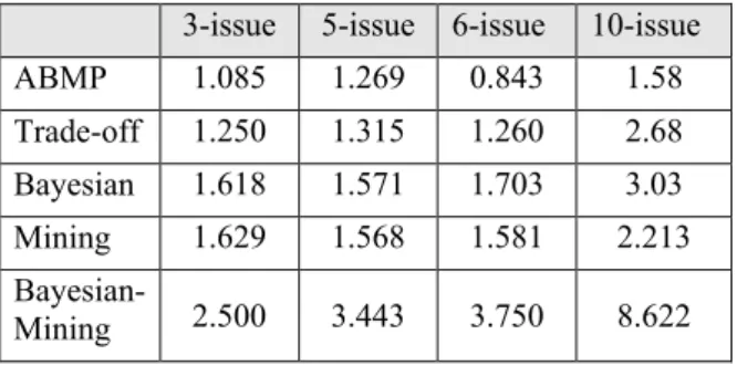
Table 7: Average Sensitivities for all strategies
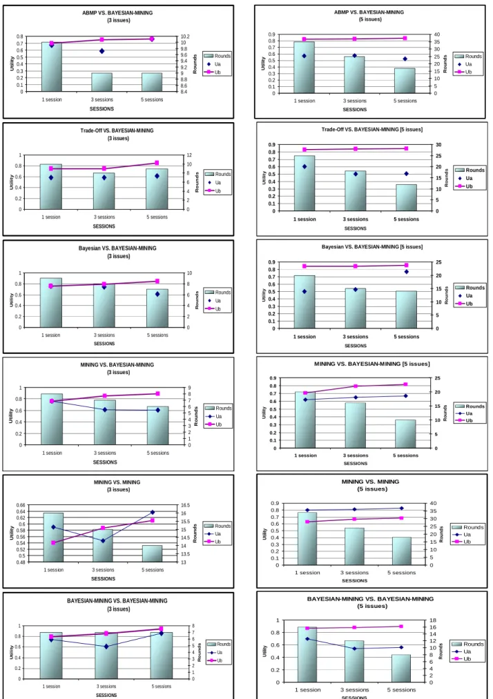
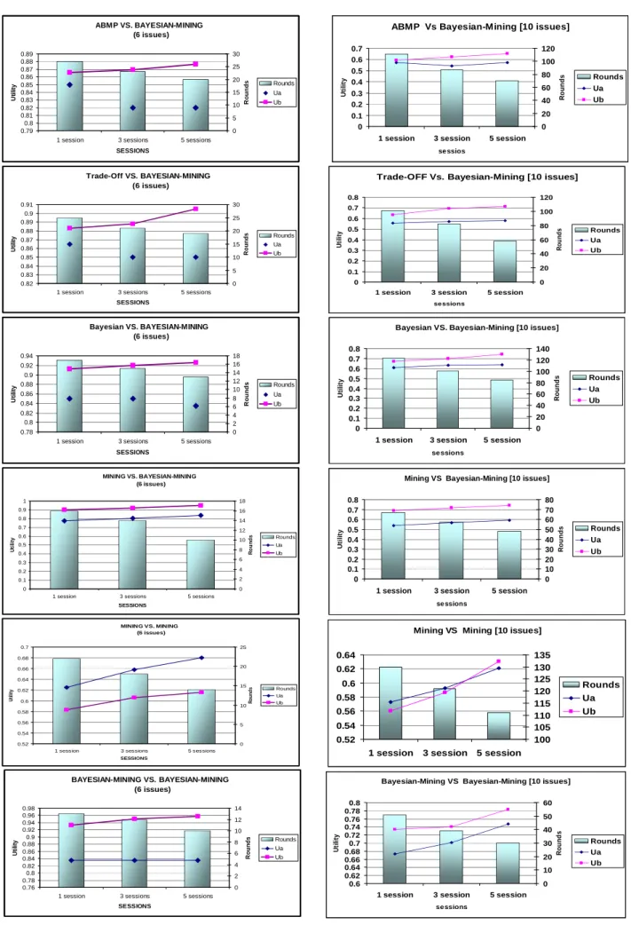
The negotiation cost is presented by the number of rounds and increase in utility. It should be noticed that single session experiments are the baseline to compare all agent strategies (Figures 5, 6, 7and 8). Additionally, in all multi-session experiments (Figures 9, 10, 11 and 12), the curves of all existing agent strategies, except for our proposed strategy, are presented only by points as they never have previous session knowledge to shorten the negotiation rounds thus the related experiments are independent. To sum up the results, the following points may be stated.
In all Bayesian–mining experiments, the agent
wins its opponent from the first session. It gains more experience through negotiation steps and sessions such that gradually its utility is increased and the session rounds are decreased. For example, when Agent B follows Bayesian–mining and plays against an opponent Agent A which follows ABMP on 5-issue data set (Figure 10), Agent B utilities outcomes are (0.825, 0.83, 0.842) and the game session rounds are (35, 25, 17) in 1, 3 and 5 sessions respectively. Moreover, when the opponent agent A is Bayesian on 6-issue data set (Figure 11), Agent B utilities are (0.9125, 0.92, 0.92566) and the game session rounds are (17, 15, 13) in 1, 3 and 5 sessions respectively. One may notice that the first session between these parties has 17 rounds only, which are less than 29 rounds of Bayesian (Agent A) vs. Bayesian (Agent B) single session experiment (Figure 7).
All other opponents (agent A) gain from playing
with a Bayesian–mining agent (agent B). For example, agent A which follows ABMP (Figure 6) on 5-issue data set gets session rounds (75, 57, 43, 35) vs. Agent B which follows ABMP, Trade-Off, Bayesian, Bayesian–mining respectively. Also, the Trade-Off fastest single-session agreements (Figures 5, 6 and 7) occurred with the Bayesian– mining agent; 9 session rounds (3-issue data set) and 25 session rounds (5-issue and 6-issue data set).
The Bayesian–mining agent outcomes (agent B) in
all its experiments on 3-issue, 5-issue, 6-issue and 10-issue data sets effectively prove its principles.
It is illustrated that the Bayesian–mining approach
has less offers to reach rapidly the final agreement and the final utility. In most cases, especially in 10-issue experiments, it raises the opponent
utilities. The Bayesian–mining approach works with larger number of sessions having several issues as the accumulated knowledge becomes valuable.
It is noticed that in terms of the overall negotiation
quality and number of proposals exchanged to reach an agreement, the Bayesian–mining approach outperformed the other strategies. This confirmed the intuition that building mining and learning capability into agents help the agents to work more accurate with its opponent with better performance and less expensive process.
7.2.3 Sensitivity analysis
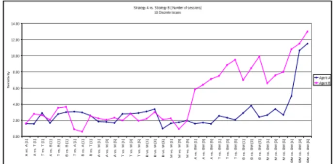
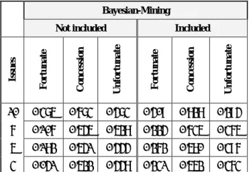
The sensitivity analysis is interested only in the negotiation intra-transaction. Table 7 summarizes the average sensitivity for all negotiation strategies used in this research. Figures 13, 14, 15 and 16 illustrate the values of this study for all the negotiation experiments.
The average sensitivity for the Bayesian-mining strategy is greater than all other strategies, which is also influenced by the preferences’ alternatives of each kind of issue (Table 7). In 3-issue experiments, the sensitivity increment ratio between Bayesian-mining (2.50) and the second highest sensitivity, i.e. Mining approach, (1.629) is 53%. In 5-issue experiments, the sensitivity increment ratio between Bayesian-mining (3.443) and second highest sensitivity, i.e. Bayesian approach, (1.571) is 119%. In 6-issue experiments, the sensitivity increment ratio between Bayesian-mining (3.750) and the second highest sensitivity, i.e. Bayesian approach, (1.703) is 120%. In all 10-issue experiments, the sensitivity increment ratio between Bayesian-mining (8.622) and the second highest sensitivity, i.e. Bayesian approach (3.03) is 184%. Figures 13, 14, 15 and 16 show that the sensitivity has increased after the first session due to the nature of the Bayesian-mining strategy which ranks the proposed offers during the session at the end of each session; the higher sensitivity value means that the agent who owns the related strategy has more information about the behaviour and the weights of preferences which the opponent gives to the issues.
In the sensitivity deep analysis, it can be found that for 3-issue, the Bayesian–mining approach sensitivity is between 2 and 4, but for other agent strategies, the sensitivity is between 0.667 and 2. For 5-issue, the Bayesian–mining approach is between 1.4 and 6, but for other agent strategies, the sensitivity is between 1.0 and 2.33. For 6-issue, the Bayesian–mining approach sensitivity is between 2.143 and 7, but for other agent strategies, the sensitivity is between 0.5 and 2.50. For 10-issue, the Bayesian–mining approach strategy is between 5.824 and 13, but for other agent strategies, the sensitivity is between 0.915 and 4.058.
To sum up the sensitivity results, the following points should be clarified:
Increasing the issues number leads to increasing
the sensitivity values of all strategies, because the
3-issue 5-issue 6-issue 10-issue
ABMP 1.085 1.269 0.843 1.58
Trade-off 1.250 1.315 1.260 2.68
Bayesian 1.618 1.571 1.703 3.03
Mining 1.629 1.568 1.581 2.213