When comparing independent groups researchers often analyze the means by performing a Student’s t-test or classical Analysis of Variance (ANOVA) F-test (Erceg-Hurn & Mirosevich, 2008; Keselman et al., 1998; Tomarken & Serlin, 1986). Both tests rely on the assumptions that independent and identically distributed residuals (1) are sampled from a normal distribution and (2) have equal variances between groups (or homoscedasticity; see Lix, Keselman, & Keselman, 1996). While a deviation from the normality assumption generally does not strongly affect either the Type I error rates (Glass, Peckham, & Sanders, 1972; Harwell, Rubinstein, Hayes, & Olds, 1992; Tiku, 1971) or the power of the F-test (David & Johnson, 1951; Harwell et al., 1992; Srivastava, 1959; Tiku, 1971), the F-test is not robust against unequal variances (Grissom, 2000). Unequal variances can alter both the Type I error rate (David & Johnson, 1951; Harwell et al., 1992) and statistical power (Nimon, 2012; Overall, Atlas, & Gibson, 1995) of the F-test.
Although it is important to make sure test assumptions are met before a statistical test is performed, research-ers rarely provide information about test assumptions when they report an F-test. We examined statistical tests reported in 116 articles in the Journal of Personality and Social Psychology published in 2016. Fourteen percent of these articles reported a one-way F-test, but only one article indicated that the homogeneity of variances assumption was taken into account. They reported cor-rected degrees of freedom for unequal variances, which could signal the use of the W-test instead of the classical F-test. A similar investigation (Hoekstra, Kiers & Johnson, 2012) yielded conclusions about the lack of attention to both the homoscedasticity and the normality assump-tions. Despite the fact that the F-test is currently used by default, better alternatives exist, such as the Welch’s W ANOVA (W-test), the Alexander-Govern test, James’ sec-ond order test, and the Brown-Forsythe ANOVA (F*-test). Although not the focus of the current article, additional tests exist that allow researchers to compare groups either based on other estimators of central tendency than the mean (see for example Erceg-Hurn & Mirosevich, 2008; Wilcox, 1998), or based on other relevant parameters of distribution than the central tendency, such as standard deviations and the shape of the distribution (Grissom, 2000; Tomarken & Serlin, 1986). However, since most
Psychology, 32(1): 13, 1–12. DOI: https://doi.org/10.5334/irsp.198
* Université Libre de Bruxelles, Service of Analysis of the Data (SAD), Bruxelles, BE
† Eindhoven University of Technology, Human Technology
Interaction Group, Eindhoven, NL
Corresponding author: Marie Delacre ([email protected])
RESEARCH ARTICLE
Taking Parametric Assumptions Seriously: Arguments for
the Use of Welch’s
F-test instead of the Classical F-test
in One-Way ANOVA
Marie Delacre
*, Christophe Leys
*, Youri L. Mora
*and Daniël Lakens
†Student’s t-test and classical F-test ANOVA rely on the assumptions that two or more samples are independent, and that independent and identically distributed residuals are normal and have equal variances between groups. We focus on the assumptions of normality and equality of variances, and
argue that these assumptions are often unrealistic in the field of psychology. We underline the current
lack of attention to these assumptions through an analysis of researchers’ practices. Through Monte Carlo simulations, we illustrate the consequences of performing the classic parametric F-test for ANOVA when the test assumptions are not met on the Type I error rate and statistical power. Under realistic deviations from the assumption of equal variances, the classic F-test can yield severely biased results and lead to invalid statistical inferences. We examine two common alternatives to the F-test, namely the Welch’s ANOVA (W-test) and the Brown-Forsythe test (F*-test). Our simulations show that under a range of realistic scenarios, the W-test is a better alternative and we therefore recommend using the W-test by default when comparing means. We provide a detailed example explaining how to perform the W-test in SPSS and R. We summarize our conclusions in practical recommendations that researchers can use to improve their statistical practices.
researchers currently generate hypotheses about differ-ences between means (Erceg-Hurn & Mirosevich, 2008; Keselman et al., 1998), we think that a first realistic first step towards progress would be to get researchers to cor-rectly test the hypothesis they are used to.
Although the debate surrounding the assumptions of the F-test has been widely explored (see for example the meta-analysis of Harwell et al., 1992), applied research-ers still largely ignore the consequences of assumption violations. Non-mathematical pedagogical papers sum-marizing the arguments seem to be lacking from the lit-erature, and the current paper aims to fill this gap. We will discuss the pertinence of the assumptions of the F-test, and focus on the question of heteroscedasticity (that, as we will see, can have major consequences on error rates). We will provide a non-mathematical explanation of how alternatives to the classical F-test cope with heteroscedas-ticity violations. We conducted simulations in which we compare the F-test with the most promising alternatives. We argue that when variances are equal between groups, the W-test has nearly the same empirical Type I error rate and power as the F-test, but when variances are unequal, it provides empirical Type I and Type II error rates that are closer to the expected levels compared to the F-test. Since the W-test is available in practically all statistical software packages, researchers can immediately improve their sta-tistical inferences by replacing the F-test by the W-test. Normality and Homogeneity of Variances under Ecological Conditions
For several reasons, assumptions of homogeneity of variances and normality are always more or less violated (Glass et al., 1972). In this section we will summarize the specificity of the methods used in our discipline that can account for this situation.
Normality Assumption
It has been argued that there are many fields in psychol-ogy where the assumption of normality does not hold (Cain, Zhang & Yuan, 2017; Micceri, 1989; Yuan, Bentler & Chan, 2004). As argued by Micceri (1989), there are sev-eral factors that could explain departures from the nor-mality assumption, and we will focus on three of them: treatment effects, the presence of subpopulations, and the bounded measures underlying residuals.
First, although the mean can be influenced by the treat-ment effects, experitreat-mental treattreat-ment can also change the shape of a distribution, either by influencing the skewness, quantifying the asymmetry of the shape of the distribu-tion, and kurtosis, a measure of the tendency to produce extreme values. A distribution with positive kurtosis will have heavier tails than the normal distribution, which means that extreme values will be more likely, while a dis-tribution with negative kurtosis will have lighter tails than the normal distribution, meaning that extreme values will be less likely (Westfall, 2014; Wilcox, 2005). For example, a training aiming at reducing a bias perception of threat when being exposed to ambiguous words will not uni-formly impact the perception of all participants, depend-ing on their level of anxiety (Grey & Mathews, 2000). This
could influence the kurtosis of the distribution of bias score.
Second, prior to any experimental treatment, the pres-ence of several subpopulations may lead to departures from the normality assumptions. A subgroup might exist that is unequal on some characteristics relevant to the measurements, that are not controlled within the studied group, which results in mixed distributions. This unavoidable lack of control is inherent of our field given its complexity. As an illustration, Wilcox (2005) writes that pooling two normally-distributed popula-tions that have the same mean but different variances (e.g. normally distributed scores for schizophrenic and not schizophrenic participants) could result in distri-butions that are very similar to the normal curve, but with thicker tails. As another example, when assessing a wellness score for the general population, data may be sampled from a left-skewed distribution, because most people are probably not depressed (see Heun et al., 1999). In this case, people who suffer from depression and people who do not suffer from depression are part of the same population, which can leads to asymmetry in the distribution.
Third, bounded measures can also explain non-normal distributions. For example, response time can be very large, but never below zero, which results in right-skewed distributions. In sum, there are many common situa-tions in which normally distributed data is an unlikely assumption.
Homogeneity of Variances Assumption
Homogeneity of variances (or homoscedasticity) is a math-ematical requirement that is also ecologically unlikely (Erceg-Hurn & Mirosevich, 2008; Grissom, 2000). In a pre-vious paper (Delacre, Lakens & Leys, 2017), we identified three different causes of heteroscedasticity: the variability inherent to the use of measured variables, the variability induced by quasi-experimental treatments on measured variables, and the variability induced by different experi-mental treatments on randomly assigned subjects. One additional source of variability is the presence of uniden-tified moderators (Cohen et al., 2013).
the variability will be smaller compared to a school that accepts all students.
Second, a quasi-experimental treatment can have dif-ferent impacts on variances between pre-existing groups, that can even be of theoretical interest. For example, in the field of linguistics and social psychology, Wasserman and Weseley (2009) investigated the impact of language gender structure on sexist attitudes of women and men. They tested differences between sexist attitude scores of subjects who read a text in English (i.e. a language with-out grammatical gender) or in Spanish (i.e. a language with grammatical gender). The results showed that (for a reason not explained by the authors), the women’s score on the sexism dimension was more variable when the text was read in Spanish than in English (SDspanish = .80 > SDenglish = .50). For men, the reverse was true (SDspanish = .97 < SDenglish = 1.33).1
Third, even when the variances of groups are the same before treatment (due to a complete succesful randomiza-tion in group assignment), unequal variances can emerge later, as a consequence of an experimental treatment (Box, 1954; Bryk & Raudenbush, 1988; Cumming, 2005; Erceg-Hurn & Mirosevich, 2008; Keppel & Wickens, 2004). For example, Koeser and Sczesny (2014) have compared arguments advocating either masculine generic or gen-der-fair language with control messages in order to test the impact of these conditions on the use of gender-fair wording (measured as a frequency). They report that the standard deviations increase after treatment in all experi-mental conditions.
Consequences of Assumption Violations
Assumptions violations would not be a matter per se, if the F-test was perfectly robust against departures from them (Glass et al., 1972). When performing a test, two types of errors can be made: Type I errors and Type II errors. A Type I error consists of falsely rejecting the null hypothesis in favour of an alternative hypothesis, and the Type I error rate (α) is the proportion of tests that, when sampling many times from the same population, reject the null hypothesis when there is no true effect in the population. A Type II error consists of failing to reject the null hypothesis, and the Type II error rate (β) is the propor-tion of tests, when sampling many times from the same population, that fail to reject the null hypothesis when there is a true effect. Finally, the statistical power (1 – β) is the proportion of tests, when sampling many times from the same population, that correctly reject the null hypoth-esis when there is a true effect in the population.
Violation of the Normality Assumption
Regarding the Type I error rate, the shape of the distri-bution has very little impact on the F-test (Harwell et al., 1992). When departures are very small (i.e. a kurtosis between 1.2 and 3 or a skewness between –0.4 and 0.4), the Type I error rate of the F-test is very close to expecta-tions, even with sample sizes as small as 11 subjects per group (Hsu & Feldt, 1969).
Regarding the Type II error rate, many authors under-lined that departures from normality do not seriously
affect the power (Boneau, 1960; David & Johnson, 1951; Glass et al., 1972; Harwell et al., 1992; Srivastava, 1959; Tiku, 1971). However, we can conclude from Srivastava (1959) and Boneau (1960) that kurtosis has a slightly larger impact on the power than skewness. The effect of non-normality on power increases when sample sizes are unequal between groups (Glass et al., 1972). Lastly the effect of non-normality decreases when sample sizes increase (Srivastava, 1959).
Violation of Homogeneity of Variances Assumption
Regarding the Type I error rate, the F-test is sensitive to unequal variances (Harwell et al., 1992). More specifi-cally, the more unequal the SD of the population’s sam-ples are extracted from, the higher the impact. When there are only two groups, the impact is smaller than when there are more than two groups (Harwell et al., 1992). When there are more than two groups, the F-test becomes more liberal, meaning that the Type I error rate is larger than the nominal alpha level, even when sample sizes are equal across groups (Tomarken & Serlin, 1986). Moreover, when sample sizes are unequal, there is a strong effect of the sample size and variance pairing. In case of a positive pairing (i.e. the group with the larger sample size also has the larger variance), the test is too conservative, meaning that the Type I error rate of the test is lower than the nominal alpha level, whereas in case of a negative pairing (i.e. the group with the larger sample size has the smaller variance), the test is too lib-eral (Glass et al., 1972; Nimon, 2012; Ovlib-erall et al., 1995; Tomarken & Serlin, 1986).
Regarding the Type II error rate, there is a small impact of unequal variances when sample sizes are equal (Harwell et al., 1992), but there is a strong effect of the sample size and variance pairing (Nimon, 2012; Overall et al., 1995). In case of a positive pairing, the Type II error rate increases (i.e. the power decreases), and in case of a negative pairing, the Type II error decreases (i.e. the power increases).
Cumulative Violation of Normality and Homogeneity of Variance
Regarding both Type I and Type II error rates, following Harwell et al. (1992), there is no interaction between nor-mality violations and unequal variances. Indeed, the effect of heteroscedasticity is relatively constant regardless of the shape of the distribution.
The Mathematical Differences Between the F-test, W-test, and F*-test
The mathematical differences between the F-test, W-test and F*-test can be explained by focusing on how standard deviations are pooled across groups. As shown in (1) the F statistic is calculated by dividing the inter-group variance by a pooled error term, where s2j and nj are respectively the variance estimates and the sample sizes from each independent group, and where k is the number of inde-pendent groups: 2 .. 1 2 1
1 ( )
1 1
( j 1)
k j j j k j j
n x x
k F n s N k = =
é - ù
ê ú ë û -=
-å
å
(1)The degrees of freedom in the numerator (2) and in the denominator (3) of the F-test are computed as follows:
1 n
df = −k (2)
, d
df =N k− (3)
With N =∑kj=1nj. As a generalization of the Student’s t-test, the F-test is calculated based on a pooled error term. This implies that all samples are considered as issued from a common population variance (hence the assumption of homoscedasticity). When there is heteroscedasticity, and if the larger variance is associated with the larger sample size, the error term, which is the denominator in (1), is overestimated. The F-value is therefore smaller, leading to fewer significant findings than expected, and the F-test is too conservative. When the larger variance is associated with the smaller sample size the denominator in (1) is underestimated. The F-value is then inflated, which yields more significant results than expected.
The F* statistic proposed by Brown and Forsythe (1974) is computed as follows:
(
)
( )
2 1 2 1 ¨ * 1 j k j j j k n j N j x x n F s = = ⎡ − ⎤ ⎢ ⎥ ⎣ ⎦ = ⎡ − ⎤ ⎢ ⎥ ⎣ ⎦∑
∑
(4)Where xj and 2 j
s are respectively the group mean and the group variance, and
¨
x is the overall mean. As it can be seen in (4) the numerator of the F* statistic is equal to the sum of squares between groups (which is equal to the numerator of the F statistic when one compares two groups). In the denominator, the variance of each group is weighted by 1 minus the relative frequency of each group. This adjustment implies that the variance associated with the group with the smallest sample size is given more weight compared to the F-test. As a result, when the larger variance is associated with the larger sample size, F* is larger than F, because the denomina-tor decreases, leading to more significant findings com-pared to the F-test. On the other hand, when the larger variance is associated with the smaller sample size, F* is smaller than F, because the denominator increases,
lead-ing to fewer significant findlead-ings compared to the F-test. The degrees of freedom in the numerator and in the denominator of F*-test are computed as follows (with the same principle as the denominator computation of the F* statistic):
1
n
df = −k (5)
2 2 2 1 1 1 1 1 [ ] 1 d j j k j j j k j j df n s N n s N n = = = ⎛ ⎛ ⎞ ⎞ ⎜ ⎜ − ⎟ ⎟ ⎜ ⎝ ⎠ ⎟ ⎜ ⎡ ⎤⎟ ⎛ ⎞ ⎜ ⎢ − ⎥⎟ ⎜ ⎟ ⎜ ⎢ ⎥⎟ ⎝ ⎠ ⎣ ⎦ ⎝ ⎠ −
∑
∑
(6)Formula (7) provides the computation of the W-test, or Welch’s F-test. In the numerator of the W-test the squared deviation between group means and the general mean are weighted by 2
j j n
s instead of nj (Brown & Forsythe, 1974). As a consequence, for equal sample sizes, the group with the highest variance will have smaller weight (Liu, 2015).
(
)
(
)
2 1 2 2 1 1 12 2 1
1 1 1 1 k j j j k j j j
w X X
k W w k n w k = = ⎡ − ′ − = ⎛ ⎞ ⎛ ⎞ − + ⎜⎜ − ⎟ ⎜⎟ − ⎟ − ⎝ ⎤ ⎢ ⎥ ⎣ ⎦ ⎡ ⎤ ⎢ ⎥ ⎢ ⎥ ⎦ ⎠ ⎝ ⎣ ⎠
∑
∑
(7)where: 2 j j j n w s = 2 1 k j j j n w s = ⎛ ⎞ ⎜ ⎟ ⎜ ⎟ ⎝ ⎠ =
∑
(
)
1 j k j j w xX
w =
′ =
∑
The degrees of freedom of the W-test are approximated as follows:
1
n
df = −k (8)
2 2 1 ( 1 1 3 1 ) j d w k w j j k df n = − = ⎡ − ⎤ ⎢ ⎥ − ⎢ ⎥ ⎣ ⎦
∑
(9)Monte Carlo simulations: F-test versus W-test versus F*-test
We performed Monte Carlo simulations using R (version 3.5.0) to assess the Type I and Type II error rates for the three tests. One million datasets were generated for 3840 scenarios that address the arguments present in the litera-ture. In 2560 scenarios, means were equal across all groups (i.e. the null hypothesis is true), in order to assess the Type I error rate of the tests. In 1280 scenarios, there were dif-ferences between means (i.e. the alternative hypothesis is true) in order to assess the power of the tests. In all sce-narios, when using more than 2 samples, all samples but one was generated from the same population, and only one group had a different population mean.
Population parameter values were chosen in order to illustrate the consequences of factors known to play a key role on both the Type I error rate and the statistical power when performing an ANOVA. Based on the literature review presented above, we manipulated the number of groups, the sample sizes, the sample size ratio ( -ratio = k)
j n n
n , the
SD-ratio ( -ratio = k)
j
SD , and the sample size and variance pairing. In our scenarios, the number of compared groups (k) varied from 2 to 5. Sample sizes of k-1 groups (nj) were 20, 30, 40, 50, or 100. The sample size of the last group was a function of the n-ratio, ranging from 0.5 to 2, in steps of 0.5. The simulations for which the n-ratio equals 1 are known as a balanced design (i.e. sample sizes are equal across all groups). The SD of the population from which was extracted last group was a function of the SD-ratio, with values of 0.5, 1, 2 or 4. The simulations for which the SD-ratio equals 1 are the particular case of homoscedastic-ity (i.e. equal variances across groups).
All possible combinations of n-ratio and SD-ratio were performed in order to distinguish positive pairings (the group with the largest sample size is extracted from the population with the largest SD), negative pairings (the group with the smallest sample size is extracted from the population with the smallest SD), and no pairing (sample sizes and/or population SD are equal across all groups). All of those conditions were tested with normal and non-normal distributions. When two groups are compared, conclusions for the three ANOVA tests (F, F*, W) should yield identical error rates when compared to their equiva-lent t-tests (the F-test is equivaequiva-lent to Student’s t-test, and the F*-test and W-test are equivalent to Welch’s t-test; Delacre et al., 2017). When there are more than three groups, the F-test becomes increasingly liberal as soon as the variances of the distributions in each group are not similar, even when sample sizes are equal between groups (Harwell et al., 1992; Quensel, 1947).
For didactic reasons, we will report only the results where we compared three groups (k = 3). Increasing the number of groups increases how liberal all tests are. For interested readers, all figures for cases where we compare more than three groups are available here: https://osf. io/h4ks8/. Overall, the larger the sample sizes, the less the distributions of the population underlying the sam-ples impact the robustness of the tests (Srivastava, 1959). However, increasing the sample sizes does not improve the robustness of the test when there is heteroscedasticity.
Interested reader can see all details in the following Excel spreadsheet, available on github: « Type I error rate.xlsx ».
In sum, the simulations grouped over different sample sizes yield 9 conditions based on the n-ratio, SD-ratio, and sample size and variance pairing, as summarized in
Table 1.
In all Figures presented below, averaged results for each sub-condition are presented under seven different config-urations of distributions, using the following legend. Type I Error Rate of the F-test, W-test, and F*-test
As previously mentioned, the Type I error rate (α) is the long-run frequency of observing significant results when the null-hypothesis is true. When means are equal across all groups the Type I error rate of all test should be equal to the nominal alpha level. We assessed the Type I error rate of the F-test, W-test and F*-test under 2560 scenarios using a nominal alpha level of 5%.
When there is no difference between means, the nine cells of Table 1 simplify into five sub-conditions:
• Equal n and SD across groups (a)
• Unequal n but equal SD across groups (b and c) • Unequal SD but equal n across groups (d and g) • Unequal n and SD across groups, with positive
correlation between n and SD (e and i)
• Unequal n and SD across groups, with negative correlation between n and SD (f and h)
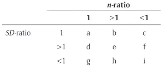
Table 1: 9 conditions based on the n-ratio, SD-ratio, and sample size and variance pairing.
n-ratio
1 >1 <1
SD-ratio 1 a b c
>1 d e f
<1 g h i
Note: The n-ratio is the sample size of the last group divided by the sample size of the first group. When all sample sizes are equal across groups, the n-ratio equals 1. When the sample size of the last group is higher than the sample size of the first group, n-ratio >1, and when the sample size of the last group is smaller than the sample size of the first group, n-ratio <1. SD-ratio is the population SD of the last group divided by the population SD of the first group. When all samples are extracted from populations with the same SD, the SD-ratio equals 1. When the last group is extracted from a population with a larger SD than all other groups, the SD-ratio >1. When the last group is extracted from a population with a smaller SD than all other groups, the SD-ratio <1.
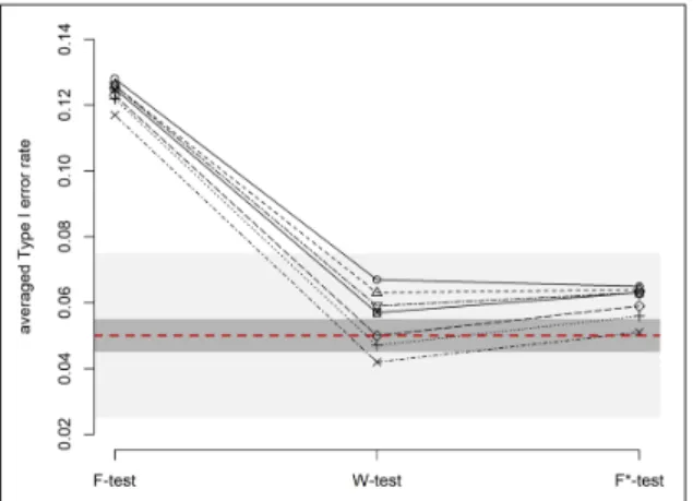
In Figures 2 to 6 (see Figure 1 for the legend), we com-puted the average Type I error rate of the three tests under these five subcategories. The light grey area corresponds to the liberal criterion from Bradley (1978), who regards a departure from the nominal alpha level as acceptable whenever the Type I error rate falls within the interval [0.5 × α; 1.5 × α]. The dark grey area corresponds to the more conservative criterion from which departures from the nominal alpha is considered negligible as long as the Type I error rate falls within the interval [0.9 × α; 1.1 × α].
In Figures 2 and 3 (cells a, b, and c in Table 1), the pop-ulation variance is equal between all groups, so the homo-scedasticity assumption is met. The F-test and F*-test only marginally deviate from the nominal 5%, regardless of the underlying distribution and the SD-ratio. The W-test also only marginally deviates from the nominal 5%, except under asymmetry (the tests becomes a little more liberal) or extremely heavy tails (the test becomes a bit more con-servative), consistently with observations in Harwell et al. (1992). However, deviations don’t exceed the liberal crite-rion of Bradley (1978).
In Figures 4, 5 and 6 (cells d to i, Table 1) the popu-lation variance is unequal between groups, so that the homoscedasticity assumption is not met. When sample sizes are equal across groups (Figure 4) and when there is a positive correlation between sample sizes and SDs (Figure 5), the Type I error rate of the W-test is closer to the nominal 5% than the Type I error rate of the F*-test and the F-test, the latter which is consistently at the lower limit of the liberal interval suggested by Bradley, in line with Harwell et al. (1992), Glass et al. (1972), Nimon (2012) and Overall et al. (1995). Heteroscedasticity does not impact the Type I error rate of the W-test, regardless of the distribution (the order of the distribution shape remains the same in all conditions).
When there is a negative correlation between sample sizes and SDs (Figure 6), the Type I error rate of the F*-test is slightly closer of the nominal 5% than the Type I error rate of the W-test, for which the distributions (more spe-cifically, the skewness) has a larger impact on the Type I error rate than when there is homoscedasticity. This is consistent with conclusions of Lix et al. (1996) about
Figure 2: Type I error rate of the F-test, W-test and F*-test when there are equal SDs across groups and equal sample sizes (cell a in Table 1).
Figure 3: Type I error rate of the F-test, W-test and F*-test when there are equal SDs across groups and unequal sample sizes (cells b and c in Table 1).
Figure 4: Type I error rate of the F-test, W-test and F*-test when there are unequal SDs across groups and equal sample sizes (cells d and g in Table 1).
the Alexander-Govern and the James’ second order tests (which return very similar results as the W-test, as we already mentioned). However, both tests still perform rela-tively well, contrary to the F-test that is much too liberal, in line with observations by Harwell et al. (1992), Glass et al. (1972), Nimon (2012) and Overall et al. (1995).
Conclusions
We can draw the following conclusions for the Type I error rate:
1) When all assumptions are met, all tests perform ad-equately.
2) When variances are equal between groups and dis-tributions are not normal, the W-test is a little less efficient than both the F-test and the F*-test, but de-partures from the nominal 5% Type I error rate never exceed the liberal criterion of Bradley (1978). 3) When the assumption of equal variances is
violat-ed, the W-test clearly outperforms both the F*-test (which is more liberal) and the F-test (which is either more liberal or more conservative, depending on the SDs and SD pairing).
4) The last conclusion generally remains true when both the assumptions of equal variances and nor-mality are not met.
Statistical power for the F-test, W-test, and F*-test
As previously mentioned, the statistical power (1 – β) of a test is the long-run probability of observing a statistically significant result when there is a true effect in the popula-tion. We assessed the power of the F-test, W-test and F*-test under 1280 scenarios, while using the nominal alpha level of 5%. In all scenarios, the last group was extracted from a population that had a higher mean than the population from where were extracted all other groups (μk = μj + 1). Because of that, in some scenarios there is a positive correlation between the SD and the mean (i.e. the last group has the largest SD and the largest mean) and in other scenarios, there is a negative correlation between SD and the mean (i.e. the last group has the smallest SD
and the largest mean). As we know that the correlation between the SD and the mean matters for the W-test (see Liu, 2015), the 9 sub-conditions in Table 1 were analyzed separately.
We computed two main outcomes: the consistency and the power. The consistency refers to the relative difference between the observed power and the nominal power, divided by the expected power:
0 E
Consistency E
−
= (10)
When consistency equals zero, the observed power is consistent with the nominal power (under the paramet-ric assumptions of normality and homoscedasticity); a negative consistency shows that the observed power is lower than the expected power; and a positive consist-ency shows that the observed power is higher than the expected power.
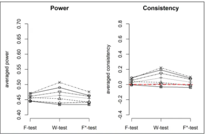
In Figures 7, 8 and 9 (cells a, b, and c in Table 1 see
Figure 1 for the legend), the population variance is equal between all groups, meaning that the homoscedastic-ity assumption is met. When distributions are normal,
Figure 6: Type I error rate of the F-test, W-test and F*-test when there are unequal SDs across groups, and negative correlation between sample sizes and SDs (cells f and g in Table 1).
Figure 7: Power and consistency of the F-test, W-test and F*-test when there are equal SDs across groups and equal sample sizes (cell a in Table 1).
the W-test is slightly less powerful than the F-test and F*-test, even though differences are very small. With all other distributions, the W-test is generally more power-ful than the F*-test and F-test, even with heavy-tailed distributions, which is in contrast with previous findings (Wilcox, 1998). Wilcox (1998) concluded that there is a loss of power when means from heavy-tailed distributions (e.g. double exponential or a mixed normal distribution) are compared to means from normal distributions. This finding is based on the argument that heavy-tailed dis-tributions are associated with bigger standard deviations than normal distributions, and that the effect size for such distributions is therefore smaller (Wilcox, 2011). However, this conclusion is based on a common conflation of kur-tosis and the standard deviation, which are completely independent (DeCarlo, 1997). One can find distributions that have similar SD but different kurtosis (see Appendix 2). However, while the W-test is more powerful than the F-test and the F*-test in many situations, it is a bit less consistent with theoretical expectations than both other tests in the sense that the W-test is generally more power-ful than expected (especially with high kurtosis, or when asymmetries go in opposite directions). This is due to the fact that the W-test is more impacted by the distribution shape, in line with observations by Harwell et al. (1992). Note that differences between W-test and other tests, in terms of consistency, are very small.
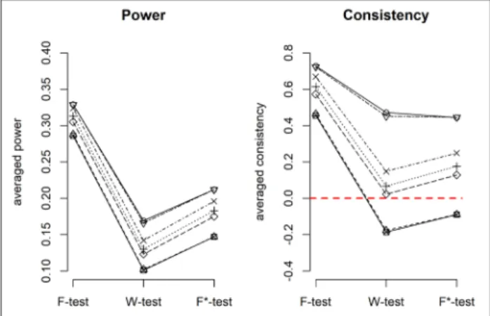
In Figures 10 to 15 (cells d to i in Table 1 see
Figure 1 for the legend), the population variance is une-qual between groups, meaning that the homoscedastic-ity assumption is not met. When sample sizes are equal across groups (Figures 10 and 11), the F-test and the F*-tests are equally powerful, and have the same con-sistency, whatever the correlation between the SD and the mean. On the other hand, the power of the W-test depends on the correlation between the SD and the mean (in line with Liu, 2015). When the group with the larg-est mean has the larglarg-est variance (Figure 10), the largest deviation between group means and the general mean is given less weight, and as a consequence the W-test is less powerful than both other tests. At the same time, the test is slightly less consistent than both other tests. When the group with the largest mean has the smallest variance
(Figure 11), the largest deviation between group means and the general mean is given more weight, and therefore the W-test is more powerful than both other tests. The test is also slightly more consistent than both other tests.
When sample sizes are unequal across groups, the power of the F*-test and the F-test are a function of the correlation between sample sizes and SDs. When there is a negative correlation between sample sizes and SDs (Figures 12 and 13), the F-test is always more powerful than the F*-test. Indeed, as was explained in the previous mathematical section, the F-test gives more weight to the smallest variance (the statistic is therefore increased) while the F*-test gives more weight to the largest variance (the statistic is therefore decreased). Conversely, when there is a positive correlation between sample sizes and SDs (Figures 14 and 15), the F-test is always more con-servative than the F*-test, because the F-test gives more weight to the largest variance while the F*-test gives more weight to the smallest variance.
The power of the W-test is not a function of the correla-tion between sample sizes and SDs, but rather a funccorrela-tion of the correlation between SDs and means. The test is more powerful when there is a negative correlation between SDs and means, and less powerful when there is a positive
Figure 9: Power and consistency of the F-test, W-test and F*-test when there are equal SDs across groups, and negative correlation between sample sizes and means (cell c in Table 1).
Figure 10: Power and consistency of the F-test, W-test and F*-test when there are unequal SDs across groups, positive correlation between SDs and means, and equal sample sizes across groups (cell d in Table 1).
correlation between SDs and means. Note that for all tests, the effect of heteroscedasticity is approximately the same regardless of the shape of the distribution. Moreover,
there is one constant observation in our simulations: whatever the configuration of the n-ratio, the consistency of the three tests is closer to zero when there is a negative correlation between the SD and the mean (meaning that the group with the highest mean has the lower variance).
We can draw the following conclusions about the statis-tical power of the three tests:
1) When all assumptions are met, the W-test falls slightly behind the F-test and the F*-test, both in terms of power and consistency.
2) When variances are equal between groups and distributions are not normal, the W-test is slightly more powerful than both the F-test and the F*-test, even with heavy-tailed distributions.
3) When the assumption of equal variances is violated, the F-test is either too liberal or too conservative, depending on the correlation between sample sizes and SDs. On the other side, the W-test is not influ-enced by the sample sizes and SDs pairing. However, it is influenced by the SD and means pairing. 4) The last conclusion generally remains true when
both assumptions of equal variances and normality are not met.
Recommendations
Taking both the effects of the assumption violations on the alpha risk and on the power, we recommend using the W-test instead of the F-test to compare groups means. The F-test and F*-test should be avoided, because a) the equal variances assumption is often unrealistic, b) tests of the equal variances assumption will often fail to detect differences when these are present, c) the loss of power when using the W-test is very small (and often even neg-ligible), and d) the gain in Type I error control is consider-able under a wide range of realistic conditions. Also, we recommend the use of balanced designs (i.e. same sample sizes in each group) whenever possible. When using the W-test, the Type I error rate is a function of criteria such as the skewness of the distributions, and whether skewness is combined with unequal variances and unequal samples sizes between groups. Our simulations show that the Type
Figure 12: Power and consistency of the F-test, W-test and F*-test when there are unequal SDs across groups, negative correlation betwen sample sizes and SDs, and positive correlation between SDs and means (cell f in Table 1).
Figure 13: Power and consistency of the F-test, W-test and F*-test when there are unequal SDs across groups, negative correlation betwen sample sizes and SDs, and negative correlation between SDs and means (cell h in Table 1).
Figure 14: Power and consistency of the F-test, W-test and F*-test when there are unequal SDs across groups, positive correlation betwen sample sizes and SDs, and positive correlation between SDs and means (cell e in Table 1).
I error rate control is in general slightly better with bal-anced designs.
Note that the W-test suffers from limitations and can-not be used in all situations. First, as previously men-tioned, W-test, as all tests based on means, does not allow researchers to compare other relevant parameters of a distribution than the mean. For these reason, we recommend to never neglect the descriptive analysis of the data. A complete description of the shape and char-acteristics of the data (e.g. histograms and boxplots) is important. When at least one statistical parameter relat-ing to the shape of the distribution (e.g. variance, skew-ness, kurtosis) seems to vary between groups, comparing results of the W-test with results of a nonparametric procedure is useful in order to better understand the data. Second, with small sample sizes (i.e. less than 50 observations per group when comparing at most four groups, 100 observations when comparing more than four groups), the W-test will not control Type I error rate when skewness is present and detecting departures for normality is therefore especially important in small samples. Unless you have good reasons to believe that distributions underlying the data have small kurtosis and skewness, we recommend to avoid alternative tests that are based on means comparison, in favour of alter-natives such as the trimmed means test (Erceg-Hurn & Mirosevich, 2008)2 or nonparametric tests. For more information about robust alternatives that are based on other parameters than the mean, see Erceg-Hurn and Mirosevich (2008).
Notes
1 Note that this is a didactic example, the differences have not been tested and might not differ statistically. 2 The null hypothesis of the trimmed means test
assumes that trimmed means are the same between groups. A trimmed mean is a mean computed on data after removing the lowest and highest values of the distribution. Trimmed means and means are equal when data are symmetric. On the other hand, when data are asymmetric, trimmed means and means differ.
Additional File
The additional file for this article can be found as follows: • Supplemental Materials. A numerical example of
the mathematical development of the F-test, W-test, and F*-test (Appendix 1) and justification for the choice of distributions in simulation (Appendix 2). DOI: https://doi.org/10.5334/irsp.198.s1
Competing Interests
The authors have no competing interests to declare. Author Contribution
The first author performed simulations. The first, sec-ond and fourth authors contributed to the design. All authors contributed to the writing and the review of the literature. The Supplemental Material, including the full
R code for the simulations and plots can be obtained from https://github.com/mdelacre/W-ANOVA. This work was supported by the Netherlands Organization for Scientific Research (NWO) VIDI grant 452-17-013. The authors declare that they have no conflicts of interest with respect to the authorship or the publication of this article.
References
Adams, B. G., Van de Vijver, F. J., de Bruin, G. P., & Bueno Torres, C. (2014). Identity in descriptions of others across ethnic groups in South Africa. Journal of Cross-Cultural Psychology, 45(9), 1411–1433. DOI: https://doi.org/10.1177/0022022114542466 Beilmann, M., Mayer, B., Kasearu, K., & Realo, A. (2014).
The relationship between adolescents’ social capital and individualism-collectivism in Estonia, Germany, and Russia. Child Indicators Research, 7(3), 589–611. DOI: https://doi.org/10.1007/s12187-014-9232-z Boneau, C. (1960). The effects of violations of
assump-tions underlying the t test. Psychological Bulle-tin, 57(1), 49–64. DOI: https://doi.org/10.1037/ h0041412
Box, G. (1954). Some theorems on quadratic forms applied in the study of analysis of variance problems, i. Effect of inequality of variance in the one-way clas-sification. The Annals of Mathematical Statistics, 25(2), 290–302. DOI: https://doi.org/10.1214/ aoms/1177728786
Bradley, J. V. (1978). Robustness? British Journal of Math-ematical and Statistical Psychology, 31(2), 144–152. DOI: https://doi.org/10.1111/j.2044-8317.1978. tb00581.x
Brown, M. B., & Forsythe, A. B. (1974). Robust tests for the equality of variances. Journal of the Ameri-can Statistical Association, 69(346), 364–367. DOI: https://doi.org/10.2307/2285659
Bryk, A. S., & Raudenbush, S. W. (1988). Hetero-geneity of variance in experimental studies: A challenge to conventional interpretations. Psycho-logical Bulletin, 104(3), 396–404. DOI: https://doi. org/10.1037/0033-2909.104.3.396
Cain, M. K., Zhang, Z., & Yuan, K.-H. (2017). Univariate and multivariate skewness and kurtosis for measur-ing nonnormality: Prevalence, influence and estima-tion. Behavior Research Methods, 49(5), 1716–1735. DOI: https://doi.org/10.3758/s13428-016-0814-1 Church, A. T.,Willmore, S. L., Anderson, A. T., Ochiai,
M., Porter, N., Mateo, N. J., Ortiz, F. A., et al. (2012). Cultural differences in implicit theories and self-perceptions of traitedness: Replication and extension with alternative measurement formats and cultural dimensions. Journal of Cross-Cultural Psychology, 43(8), 1268–1296. DOI: https://doi. org/10.1177/0022022111428514
Cohen, J., Cohen, P., West, S. G., & Aiken, L. S. (2013). Applied multiple regression/correlation analysis for the behavioural sciences. Mahwah, NJ: Erlbaum. DOI: https://doi.org/10.4324/9780203774441
Cumming, G. (2005). Understanding the new statistics: Effect sizes, confidence intervals, and meta-analysis. New York, NY: Routledge.
David, F. N., & Johnson, N. L. (1951). The effect of non-normality on the power function of the f-test in the analysis of variance. Biometrika, 38(1–2), 43–57. DOI: https://doi.org/10.2307/2332316
DeCarlo, L. T. (1997). On the meaning and use of kurtosis. Psychological Methods, 2(3), 292–307. DOI: https:// doi.org/10.1037//1082-989X.2.3.292
Delacre, M., Lakens, D., & Leys, C. (2017). Why psy-chologists should by default use Welch’s t-test instead of student’s t-test. International Review of Social Psychology, 30(1), 92–101. DOI: https://doi. org/10.5334/irsp.82
Erceg-Hurn, D. M., & Mirosevich, V. M. (2008). Modern robust statistical methods: An easy way to maximize the accuracy and power of your research. American Psychologist, 63(7), 591–601. DOI: https://doi. org/10.1037/0003-066X.63.7.591
Glass, G. V., Peckham, P. D., & Sanders, J. R. (1972). Con-sequences of failure to meet assumptions underlying the fixed effects analyses of variance and covariance. Review of Educational Research, 42(3), 237–288. DOI: https://doi.org/10.3102/00346543042003237 Green, E. G., Deschamps, J.-C., & Páez, D. (2005).
Variation of individualism and collectivism within and between 20 countries: A typo-logical analysis. Journal of Cross-Cultural Psy-chology, 36(3), 321–339. DOI: https://doi. org/10.1177/0022022104273654
Grey, S., & Mathews, A. (2000). Effects of training on interpretation of emotional ambiguity. The Quarterly Journal of Experimental Psychology, 53(4), 1143– 1162. DOI: https://doi.org/10.1080/713755937 Grissom, R. (2000). Heterogeneity of variance in
clinical data. Journal of Consulting and Clini-cal Psychology, 68(1), 155–165. DOI: https://doi. org/10.1037//0022-006X.68.1.155
Haar, J. M., Russo, M., Suñe, A., & Ollier-Malaterre, A. (2014). Outcomes of work-life balance on job satis-faction, life satisfaction and mental health: A study across seven cultures. Journal of Vocational Behav-ior, 85(3), 361–373. DOI: https://doi.org/10.1016/j. jvb.2014.08.010
Harwell, M. R., Rubinstein, E. N., Hayes, W. S., & Olds, C. C. (1992). Summarizing Monte Carlo results in methodological research: The one- and two-factor fixed effects anova cases. Journal of Educa-tional Statistics, 17(4), 315–339. DOI: https://doi. org/10.3102/10769986017004315
Henrich, J., Heine, S. J., & Norenzayan, A. (2010). Most people are not weird. Nature, 466, 29–29. DOI: https://doi.org/10.1038/466029a
Heun, R., Burkart, M., Maier, W., & Bech, P. (1999). Internal and external validity of the who well-being
scale in the elderly general population. Acta Psychi-atrica Scandinavica, 99(3), 171–178. DOI: https:// doi.org/10.1111/j.1600-0447.1999.tb00973.x Hoekstra, R., Kiers, H. A., & Johnson, A. (2012). Are
assumptions of well-known statistical techniques checked, and why (not)? Frontiers in Psychol-ogy, 3(137), 1–9. DOI: https://doi.org/10.3389/ fpsyg.2012.00137
Hsu, T.-C., & Feldt, L. S. (1969). The effect of limitations on the number of criterion score values on the sig-nificance level of the f-test. American Educational Research Journal, 6(4), 515–527. DOI: https://doi. org/10.3102/00028312006004515
Keppel, G., & Wickens, T. D. (2004). Design and analysis: A researcher’s handbook. Upper Saddle River, New Jersey: Prentice Hall.
Keselman, H., Huberty, C. J., Lix, L. M., Olejnik, S., Cribbie, R. A., Donahue, B., Levin, J. R., et al. (1998). Statistical practices of educational researchers: An analysis of their anova, manova, and ancova analy. Review of Educational Research, 68(3), 350–386. DOI: https://doi.org/10.3102/00346543068003350 Koeser, S., & Sczesny, S. (2014). Promoting gender-fair
language: The impact of arguments on language use, attitudes, and cognitions. Journal of Language and Social Psychology, 33(5), 548–560. DOI: https:// doi.org/10.1177/0261927X14541280
Liu, H. (2015). Comparing welch anova, a kruskal-wallis test, and traditional anova in case of heterogeneity of variance (PhD thesis). Virginia Commonwealth University.
Lix, L. M., Keselman, J. C., & Keselman, H. (1996). Consequences of assumption violations revisited: A quantitative review of alternatives to the one-way analysis of variance *f* test. Review of Educa-tional Research, 66(4), 579–619. DOI: https://doi. org/10.3102/00346543066004579
Micceri, T. (1989). The unicorn, the normal curve, and other improbable creatures. Psychologi-cal Bulletin, 105(1), 156–166. DOI: https://doi. org/10.1037/0033-2909.105.1.156
Montoya, D. Y., & Briggs, E. (2013). Shared ethnic-ity effects on service encounters: A study across three us subcultures. Journal of Business Research, 66(3), 314–320. DOI: https://doi.org/10.1016/j. jbusres.2011.08.011
Nimon, K. F. (2012). Statistical assumptions of substan-tive analyses across the general linear model: A mini-review. Frontiers in Psychology, 3(322), 1–5. DOI: https://doi.org/10.3389/fpsyg.2012.00322 Overall, J. E., Atlas, R. S., & Gibson, J. M. (1995). Tests
that are robust against variance heterogeneity in k × 2 designs with unequal cell frequencies. Psycho-logical Reports, 76(3), 1011–1017. DOI: https://doi. org/10.2466/pr0.1995.76.3.1011
Schneider, P. J., & Penfield, D. A. (1997). Alexander and Govern’s approximations: Providing an alternative to anova under variance heterogeneity. The Journal of Experimental Education, 65(3), 271–286. DOI: https://doi.org/10.1080/00220973.1997.9943459 Srivastava, A. B. L. (1959). Effects of non-normality on the
power of the analysis of variance test. Biometrika, 46(1– 2), 114–122. DOI: https://doi.org/10.2307/2332813 Tiku, M. (1971). Power function of the f-test under
non-normal situations. Journal of the American Statistical Association, 66, 913–916. DOI: https://doi.org/10.1 080/01621459.1971.10482371
Tomarken, A. J., & Serlin, R. C. (1986). Compari-son of anova alternatives under variance het-erogeneity and specific noncentrality structures. Psychological Bulletin, 99(1), 90–99. DOI: https:// doi.org/10.1037//0033-2909.99.1.90
Wasserman, B. D., & Weseley, A. J. (2009). ?’Qué? Quoi? Do languages with grammatical gender pro-mote sexist attitudes? Sex Roles, 61, 634–643. DOI: https://doi.org/10.1007/s11199-009-9696-3
Westfall, P. H. (2014). Kurtosis as peakedness, 1905–2014. R.I.P. The American Statistician, 68(3), 191–195. DOI: https://doi.org/10.1080/00031305 .2014.917055
Wilcox, R. R. (1998). How many discoveries have been lost by ignoring modern statistical methods? Ameri-can Psychologist, 53(3), 300–314. DOI: https://doi. org/10.1037/0003-066X.53.3.300
Wilcox, R. R. (2005). Comparing medians: An overview plus new results on dealing with heavy-tailed dis-tributions. The Journal of Experimental Education, 73(3), 249–263. DOI: https://doi.org/10.3200/ JEXE.73.3.249-263
Wilcox, R. R. (2011). Introduction to robust estimation and hypothesis testing. Cambridge, Massachusetts, US: Academic Press. DOI: https://doi.org/10.1016/ B978-0-12-386983-8.00010-X
Yuan, K.-H., Bentler, P. M., & Chan, W. (2004). Structural equation modeling with heavy tailed distributions. Psychometrika, 69(3), 421–436. DOI: https://doi. org/10.1007/BF02295644
How to cite this article: Delacre, M., Leys, C., Mora, Y. L., & Lakens, D. (2019). Taking Parametric Assumptions Seriously: Arguments for the Use of Welch’s F-test instead of the Classical F-test in One-Way ANOVA. International Review of Social Psychology, 32(1): 13, 1–12. DOI: https://doi.org/10.5334/irsp.198
Submitted: 05 June 2018 Accepted: 20 May 2019 Published: 01 August 2019
Copyright: © 2019 The Author(s). This is an open-access article distributed under the terms of the Creative Commons Attribution 4.0 International License (CC-BY 4.0), which permits unrestricted use, distribution, and reproduction in any medium, provided the original author and source are credited. See http://creativecommons.org/licenses/by/4.0/.