Stochastic Differential Equations: Models and Numerics - Free Computer, Programming, Mathematics, Technical Books, Lecture Notes and Tutorials

(1)

Stochastic Differential Equations:

Models and Numerics

1

Jesper Carlsson Kyoung-Sook Moon Anders Szepessy Ra´ul Tempone Georgios Zouraris

February 12, 2019

(2)

Introduction to Mathematical

Models and their Analysis

The goal of this course is to give useful understanding for solving problems formulated by stochastic differential equations models in science, engineering, mathematical finance and machine learning. Typically, these problems require numerical methods to obtain a solution and therefore the course focuses on basic understanding of stochastic and partial differential equations to construct reliable and efficient computational methods.

Stochastic and deterministic differential equations are fundamental for the modeling in Science and Engineering. As the computational power increases, it becomes feasible to use more accurate differential equation models and solve more demanding problems: for instance to determine input data from fundamental principles, to optimally reconstruct input data using measurements or to find the optimal construction of a design. There are therefore two interesting computational sides of differential equations:

– the forward problem, to accurately determine solutions of differential equations for given data with minimal computational work and prescribed accuracy, and

– the inverse problem, to determine the input data for differential equations, from optimal estimates, based either on measurements or on computations with a more fundamental model.

The model can be stochastic by different reasons:

– if calibration of data implies this, as in financial mathematics, or

– if fundamental microscopic laws generate stochastic behavior when coarse-grained, as in molecular dynamics for chemistry, material science and biology, or

(6)

An understanding of which model and method should be used in a particular situation requires some knowledge of both the model approximation error and the discretization error of the method. The optimal method clearly minimizes the computational work for given accuracy. Therefore it is valuable to know something about computational accuracy and work for different numerical models and methods, which lead us to error estimates and convergence results. In particular, our study will take into account the amount of computational work for alternative mathematical models and numerical methods to solve a problem with a given accuracy.

1.1 Noisy Evolution of Stock Values

Let us consider a stock value denoted by the time dependent function S(t).To begin our discussion, assume thatS(t) satisfies the differential equation

dS

dt =a(t)S(t), which has the solution

S(t) =eR0ta(u)duS(0).

Our aim is to introduce some kind of noise in the above simple model of the form a(t) =r(t)+”noise”,taking into account that we do not know precisely how the evolution will be. An example of a ”noisy” model we shall consider is the stochastic differential equation

dS(t) =r(t)S(t)dt+σS(t)dW(t), (1.1)

where dW(t) will introduce noise in the evolution. To seek a solution for the above, the starting point will be the discretization

Sn+1−Sn=rnSn∆tn+σnSn∆Wn, (1.2)

where ∆Wn are independent normally distributed random variables with zero mean and

variance ∆tn, i.e. E[∆Wn] = 0 andV ar[∆Wn] = ∆tn=tn+1−tn.As will be seen later on,

equation (1.1) may have more than one possible interpretation, and the characterization of a solution will be intrinsically associated with the numerical discretization used to solve it.

We shall consider, among others, applications to option pricing problems. An European call option is a contract which gives the right, but not the obligation, to buy a stock for a fixed priceK at a fixed future timeT. The celebrated Black-Scholes model for the value f : (0, T)×(0,∞)→_Rof an option is the partial differential equation

∂tf +rs∂sf+

σ2_s2

2 ∂

2

sf =rf, 0< t < T,

f(s, T) = max(s−K,0),

(7)

where the constantsr and σ denote the riskless interest rate and the volatility respec-tively. If the underlying stock value S is modeled by the stochastic differential equation (1.1) satisfying S(t) = s, the Feynmann-Kaˇc formula gives the alternative probability

representation of the option price

f(s, t) =E[e−r(T−t)max(S(T)−K,0))|S(t) =s], (1.4)

which connects the solution of a partial differential equation with the expected value of the solution of a stochastic differential equation. Although explicit exact solutions can be found in particular cases, our emphasis will be on general problems and numerical solutions. Those can arise from discretization of (1.3), by finite difference or finite elements methods, or from Monte Carlo methods based on statistical sampling of (1.4), with a discretization (1.2). Finite difference and finite element methods lead to a discrete system of equations substituting derivatives for difference quotients, e.g.

ft≈

f(tn+1)−f(tn)

∆t ,

while the Monte Carlo method discretizes a probability space by substituting expected values with averages of finite samples, e.g. {S(T, ωj)}M_j₌₁ and

f(s, t)≈ M X

j=1

e−r(T−t)_{max(S(T, ω}

j)−K,0)

M .

Which method is best? The solution depends on the problem to solve and we will carefully study qualitative properties of the numerical methods to understand the answer.

1.2 Molecular Dynamics

An example where the noise can be derived from fundamental principles is molecular dynamics, modeling e.g. reactions in chemistry and biology. Theoretically molecular systems can be modeled by the Schr¨odinger equation

i∂tΨ =HΨ

where the unknown Ψ is a wave function depending on time t and the variables of coordinates and spins of all, M, nuclei and, N, electrons in the problem; and H is the Hamiltonian precisely defined by well known fundamental constants of nature and the Coulomb interaction of all nuclei and electrons. An important issue is its high computational complexity for problems with more than a few nuclei, due to the high dimension of Ψ which is roughly inL2₍

R3(M+N)), see [26]. Already simulation of a single water molecule requires a partial differential equation in 39 space dimensions, which is a demanding task to solve also with modern sparse approximation techniques.

(8)

corresponding to the current nuclei positions. This approximation, derived from a WKB approximation for heavy nuclei mass (see Section??), leads toab initio molecular dynamics

˙ xt=vt,

mv˙t=−V0(xt).

(1.5)

To determine the nuclei dynamics and find the electron energy (input toV) means now to solve a differential equation in R6M where at each time step the electron ground state energy needs to be determined for the current nuclei configuration xt_{, see [}₂₆_,₁₉_{]. To}

simulate large systems with many particles requires some simplification of the expensive force calculation ∂xiV involving the current positionxt∈R

3M _{of all nuclei.}

The Hamiltonian system (1.5) is often further modified. For instance, equation (1.5) corresponds to simulate a problem with the number of particles, volume and total energy held constant. Simulation of a system with constant number of particles, volume and temperature are often done by using (1.5) and regularly rescaling the kinetic energy to meet the fixed temperature constraint, using so called thermostats. A mathematically attractive alternative to approximate a system in constant temperature is to solve the Langevin-Itˆo stochastic differential equation

dxt=vtdt,

mdvt=−(V0(xt) +τ−1vt)dt+ (2kBT τ−1)1/2dWt

(1.6)

whereT is the temperature,kB the Boltzmann constant,W is a standard Wiener process

inR3M and τ is a relaxation time parameter (which can be determined from molecular dynamics simulation). The Langevin model (1.6) can be derived from the Schr¨odinger equation under certain assumptions, which is the subject of Sections??to??. If diffusion is important in the problem under study, one would like to make long simulations on times of order at least τ−1_{. A useful observation to efficiently simulate longer time is the}

fact that for τ →0+ the solution x_s/τ of the Langevin equation (1.6) converges to the solution ¯xs solving the Smoluchowski equation, also called Brownian dynamics

d¯xs =−V0(¯xs)ds+ (2kBT)1/2dW¯s, (1.7)

set in the slower diffusion time scale s=τ t. Here, for simplicity, the mass is assumed to be the same for all particles and normalized to m = 1 and ¯W is again a standard Wiener process in R3M. The Smoluchowski model hence has the advantage to be able to approximate particle systems over longer time and reducing to half the problem dimension by eliminating the velocity variables. In Section ?? we analyze the weak approximation error xs/τ *x¯s.The next step in the coarse-graining process is to derive

(9)

1.3 Optimal Control of Investments

Suppose that we invest in a risky asset, whose value S(t) evolves according to the stochastic differential equationdS(t) =µS(t)dt+σS(t)dW(t), and in a riskless assetQ(t) that evolves with dQ(t) =rQ(t)dt,r < µ. Our total wealth is thenX(t) =Q(t) +S(t) and the goal is to determine an optimal instantaneous policy of investment in order to maximize the expected value of our wealth at a given final timeT. Let the proportion of the total wealth invested on the risky asset at a given time t, α(t), be defined by α(t)X(t) = S(t), so that (1−α(t))X(t) = Q(t) with α(t) ∈ [0,1]. Then our optimal control problem can be stated as

max

α E[g(X(T))|X(t) =x]≡u(t, x),

whereg is a given function. How can we determine an optimal α? The solution of this problem can be obtained by means of a Hamilton Jacobi equation, which is in general a nonlinear partial differential equation of the form

ut+H(u, ux, uxx) = 0,

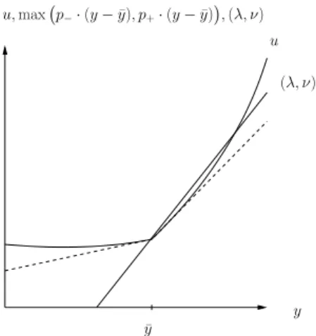
whereH(u, ux, uxx) := maxα (µαx+r(1−α)x)ux+σ2α2x2uxx/2

. Part of our work is to study the theory of Hamilton Jacobi equations and numerical methods for control problems to determine the HamiltonianH and the controlα. It turns out that typically the Hamiltonian needs to slightly modified in order to compute an approximate solution: Chapter 8 explains why and how. We call such modifications regularizations.

Chapter8 also includes a study on rare events for stochastic differential equations, e.g. the important problem of determining reaction rates and reaction path in molecular dynamics, with small noise term. The analysis of these rare events in Chapter 8 are also based on Hamilton Jacobi equations.

1.4 Calibration of the Volatility

(10)

1.5 The Coarse-graining and Discretization Analysis

Our analysis of models and discretization methods use only one basic idea, which we present here for a determinstic problem of two differential equations

˙

Xt=a(Xt)

and

˙¯

Xt= ¯a( ¯Xt).

We may think of the two given fluxes aand ¯aas either two different differential equation models or two discretization methods. The goal is to estimate a quantity of interest g(XT_{), e.g. the potential energy of a molecular dynamic system, the lift of an airfoil}

or the contract of a contingent claim in financial mathematics. Consider therefore a given function g :Rd → Rd with a solution X : [0, T] → Rd, e.g. the coordinates of atoms in a molecular system or a discretization of mass, momentum and energy of a fluid. To understand the global error g(XT₎₋_{g( ¯}_XT_{) we introduce the value function}

¯

u(x, t) :=g( ¯XT_{; ¯}_Xt₌_{x), which solves the partial differential equation}

∂tu(x, t) + ¯¯ a(x)∂xu(x, t) = 0¯ t < T

u(·, T) =g (1.8)

This definition and telescoping cancellation imply that the global error has the represen-tation

g(XT₎₋_{g( ¯}_XT_{) = ¯}_u(XT_{, T}₎₋_{u( ¯}_¯ _X0

|{z}

=X0

,0)

= ¯u(XT, T)−u(X¯ 0,0)

=

Z T

0

d¯u(Xt_{, t)}

=

Z T

0

∂tu(X¯ t, t) + ˙Xt∂xu(X¯ t, t)dt

=

Z T

0

∂tu(X¯ t, t) + ¯a(Xt, t)∂xu(X¯ t, t)dt

=

Z T

0

−¯a(Xt, t) +a(Xt, t)

∂xu(X¯ t, t)dt.

(1.9)

Here we can identify the local error in terms of the residual−¯a(Xt_{, t)+ ¯}_a(Xt_{, t) multiplied}

by the weight ∂xu(X¯ t, t) and summed over all time steps. Note that the difference of

the two solutions in the global error is converted into a weighted average of the residual

−¯a(Xt_{, t) + ¯}_a(Xt_{, t) along only one solution} _Xt_{; the representation is therefore the}

residual ofX-path inserted into the ¯u-equation. We may view the error representation as a weak form of Lax Equivalence result, which states that the combination of consistence and stability imply convergence: consistence means that the flux ¯a approximates a; stability means that ∂xu¯ is bounded in some sense; and convergence means that the

(11)

stated using bounds with appropriate norms and it has been the basis of the theoretical understanding of numerical methods.

The weak formulation (1.9) is easy to use and it is our basis for understanding both modelling and discretization errors. The weak form is particularly useful for estimating the weak approximation error, since it can take cancellation into account by considering the weaker concept of the value function instead of using absolute values and norms of differences of solution paths; the standard strong error analysis is obtained by estimating the norm of the difference of the two paths X and ¯X. Another attractive property of the weak representation (1.9) is that it can be applied both in a priori form to give qualitative results, by combining it with analytical estimates of∂xu, and in¯ a posteriori

form to obtain also quantitative results, by combining it with computer based estimates of ∂xu.¯

We first use the representation for understanding the weak approximation of stochastic differential equations and its time discretization, by extending the chain rule to Ito’s formula and integrate over all outcomes (i.e. take the expected value). The value function solves a parabolic diffusion equation in this case, instead of the hyperbolic transport equation (1.8).

In the case of coarse-graining and modelling error, the representation is used for approximating

– Schr¨odinger dynamics by stochastic molecular Langevin dynamics,

– Kinetic Monte Carlo jump dynamics by SDE dynamics,

– Langevin dynamics by Smoluchowski dynamics, and

– Smoluchowski molecular dynamics by continuum phase-field dynamics.

We also use the representation for the important problem to analyse inverse problems, such as callibrating the volatility for stocks by observed option prices or finding an optimal portfolio of stocks and bonds. In an optimal control setting the extension is then to include a control parameter α in the flux so that

˙

Xt=a(Xt, αt)

where the objective now is to find the minimum minαg(XT; Xt=x) =:u(x, t). Then

the value function u solves a nonlinear Hamilton-Jacobi-Bellman equation and the representation is extended by including a minimum over α.

1.6 Machine Learning

Here is first a short description of a machine learning problem to determine a neural network function from given data. For example, we are given data {(xn, yn)}Nn=1,

(12)

density on Rd×R. The objective is to train/learn a neural network function, e.g. α(x, θ) :=PK

k=1θk1σ(θ2k·x+θk3), that solves the minimization problem

min

θ∈R(d+2)K

E[f α(x, θ), y]

with the activation functionσ(y) := 1/(1 +e−y_{), the loss function} _{f(α, y) :=} _|_α₋_y_|2

and the neural network parametersθ= (θ1

k, θ2k, θk3)Kk=1 where θk1 ∈R, θ2k∈Rd andθk3 ∈R.

The stochastic gradient descent method for the iterationsθ[n]∈_R(d+2)K_{, n}_{= 0,}_1,_{2, . . .}

satisfying

θ[0] = some random guess inR(d+2)K, θ[n+ 1] =θ[n]−∆t∇_θf α(xn, θ[n]), yn

, n= 0,1,2, . . . (1.10)

is often used to approximately solve this minimization problem, based on a step size/learning rate ∆t >0. By writing the stochastic gradient descent method as

θ[0] = some random guess inR(d+2)K, θ[n+ 1] =θ[n]−∆t∇_θ_E[f α(xn, θ[n]), yn

]

+ ∆tE[∇θf α(xn, θ[n]), yn

]− ∇_θf α(xn, θ[n]), yn

, n= 0,1,2, . . .

it can be understood as a Euler approximation of a certain stochastic differential equation with drift ∇_θ_E[f α(xn, θ[n]), yn

(13)

Chapter 2

Stochastic Integrals

This chapter introduces stochastic integrals, which will be the basis for stochastic differential equations in the next chapter. Here we construct approximations of stochastic integrals and prove an error estimate. The error estimate is then used to establish existence and uniqueness of stochastic integrals, which has the interesting ingredient of intrinsic dependence on the numerical approximation due to infinite variation. Let us first recall the basic definitions of probability we will use.

2.1 Probability Background

A probability space is a triple (Ω,F, P), where Ω is the set of outcomes,F is the set of events and P :F →[0,1] is a function that assigns probabilities to events satisfying the following definitions.

Definition 2.1. If Ω is a given non empty set, then a σ-algebra F on Ω is a collection

F of subsets of Ω that satisfy:

(1) Ω∈ F;

(2) F ∈ F ⇒Fc_{∈ F}_{, where} _Fc_{= Ω}₋_F _{is the complement set of} _F _{in Ω; and}

(3) F1, F2, . . .∈ F ⇒S+_i₌₁∞Fi ∈ F.

Definition 2.2. A probability measure on (Ω,F) is a set functionP :F →[0,1] such that:

(1) P(∅) = 0, P(Ω) = 1; and

(2) IfA1, A2, . . .∈ F are mutually disjoint sets then

P

+∞

[

i=1

Ai !

=

+∞

X

i=1

(14)

Definition 2.3. A random variable X, in the probability space (Ω,F, P), is a function X : Ω→Rd such that the inverse image

X−1_(A)_{≡ {}_ω_∈_{Ω :}_X(ω)_∈_A_{} ∈ F}_,

for all open subsetsA of Rd.

Definition 2.4 (Independence of random variables). Two setsA, B ∈ F are said to be independent if

P(A∩B) =P(A)P(B).

Two independent random variablesX, Y inRd are independent if

X−1_{(A) and}_Y−1_{(B) are independent for all open sets}_{A, B}_⊆

Rd.

Definition 2.5. A stochastic process X : [0, T]×Ω → _Rd _{in the probability space}

(Ω,F, P) is a function such thatX(t,·) is a random variable in (Ω,F, P) for allt ∈(0, T). We will often write X(t)≡X(t,·).

Thet variable will usually be associated with the notion of time.

Definition 2.6. Let X : Ω → _R be a random variable and suppose that the density function

p0(x) = P(X∈dx) dx

is integrable. The expected value of X is then defined by the integral

E[X] =

Z ∞

−∞

xp0(x)dx, (2.1)

which also can be written

E[X] =

Z ∞

−∞

xdp(x). (2.2)

The last integral makes sense also in general when the density function is a measure, e.g. by successive approximation with random variables possessing integrable densities. A point mass, i.e. a Dirac delta measure, is an example of a measure.

Exercise 2.7. Show that ifX, Y are independent random variables then E[XY] =E[X]E[Y].

2.2 Brownian Motion

As a first example of a stochastic process, let us introduce

Definition 2.8(The Wiener process). The one-dimensionalWiener process W : [0,∞)×

(15)

(1) with probability 1, the mapping t7→W(t) is continuous andW(0) = 0; (2) if 0 =t0 < t1 < . . . < tN =T,then the increments

W(tN)−W(tN−1), . . . , W(t1)−W(t0)

areindependent; and

(3) for allt > sthe incrementW(t)−W(s) has thenormal distribution, withE[W(t)−

W(s)] = 0 andE[(W(t)−W(s))2_{] =}_t₋_s, _i.e.

P(W(t)−W(s)∈Γ) =

Z

Γ

e −y2

2(t−s)

p

2π(t−s)dy, Γ⊂R.

Does there exists a Wiener process and how to constructW if it does? In computations we will only need to determineW at finitely many time steps {tn: n= 0, . . . , N} of the

form 0 = t0 < t1 < . . . < tN =T. The definition then shows how to generate W(tn)

by a sum of independent normal distributed random variables, see Example 2.20 for computational methods to generate independent normal distributed random variables. These independent increments will be used with the notation ∆Wn=W(tn+1)−W(tn).

Observe, by Properties 1 and 3, that for fixed time t the Brownian motionW(t) is itself a normal distributed random variable. To generate W for all t∈_R is computationally infeasible, since it seems to require infinite computational work. Example 2.20 shows the existence of W by proving uniform convergence of successive continuous piecewise linear approximations. The approximations are based on an expansion in the orthogonal L2_{(0, T}_{) Haar-wavelet basis.}

2.3 Approximation and Definition of Stochastic Integrals

Remark 2.9 (Questions on the definition of a stochastic integral). Let us consider the problem of finding a reasonable definition for the stochastic integral RT

0 W(t)dW(t),

whereW(t) is the Wiener process. As a first step, let us discretize the integral by means of the forward Euler discretization

N−1

X

n=0

W(tn) (W(tn+1)−W(tn)))

| {z }

=∆Wn

.

Taking expected values we obtain by Property 2 of Definition2.8

E[

N−1

X

n=0

W(tn)∆Wn] = N−1

X

n=0

E[W(tn)∆Wn] = N−1

X

n=0

E[W(tn)]E[∆Wn] | {z }

=0

= 0.

Now let us use instead thebackward Euler discretization

N−1

X

n=0

(16)

Taking expected values yields a different result:

N−1

X

n=0

E[W(tn+1)∆Wn] = N−1

X

n=0

E[W(tn)∆Wn] +E[(∆Wn)2] = N−1

X

n=0

∆t=T 6= 0.

Moreover, if we use thetrapezoidal method the result is

N−1

X

n=0

E

W(tn+1) +W(tn)

2 ∆Wn

=

N−1

X

n=0

E[W(tn)∆Wn] +E[(∆Wn)2/2]

=

N−1

X

n=0

∆t

2 =T /26= 0.

Remark2.9 shows that we need more information to define the stochastic integral

Rt

0W(s)dW(s) than to define a deterministic integral. We must decide if the solution

we seek is the limit of the forward Euler method. In fact, limits of the forward Euler define the so called Itˆo integral, while the trapezoidal method yields the so called

Stratonovich integral. It is useful to define the class of stochastic processes which can be Itˆo integrated. We shall restrict us to a class that allows computable quantities and gives convergence rates of numerical approximations. For simplicity, we begin with Lipschitz continuous functions in Rwhich satisfy (2.3) below. The next theorem shows that once the discretization method is fixed to be the forward Euler method, the discretizations converge inL2_{. Therefore the limit of forward Euler discretizations is well defined, i.e.}

the limit does not depend on the sequence of time partitions, and consequently the limit can be used to define the Itˆo integral.

Theorem 2.10. Suppose there exist a positive constantC such thatf : [0, T]×_R→_R

satisfies

|f(t+ ∆t, W+ ∆W)−f(t, W)| ≤C(∆t+|∆W|). (2.3)

Consider two different partitions of the time interval [0, T]

{_t¯_n}N_n¯₌₀, ¯_t₀ _{= 0,} ¯_t_N_¯ ₌_T,

¯_¯

tm

¯ ¯

N

m=0, ¯¯t0 = 0, ¯¯tN¯¯ =T,

with the corresponding forward Euler approximations

¯ I =

¯

N−1

X

n=0

f(¯tn, W(¯tn))(W(¯tn+1)−W(¯tn)), (2.4)

¯ ¯ I =

¯ ¯

N−1

X

m=0

(17)

Let the maximum time step ∆tmax be

∆tmax= max "

max

0≤n≤N¯−1

¯

tn+1−¯tn, max

0≤m≤_N¯¯−1

¯ ¯

tm+1−t¯¯m #

.

Then

E[( ¯I−I)¯¯2] =O(∆tmax). (2.6)

Proof. It is useful to introduce the finer grid made of the union of the nodes on the two grids

{tk} ≡ {¯tn} ∪ _¯_¯

tm .

Then in that grid we can write

¯

I−I¯¯=X

k

∆fk∆Wk,

where ∆fk=f(¯tn, W(¯tn))−f(¯¯tm, W(¯¯tm)), ∆Wk=W(tk+1)−W(tk) and the indices

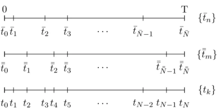
m, n satisfytk∈[¯t¯m,¯¯tm+1) andtk∈[¯tn,¯tn+1), as depicted in Figure2.1.

{tk} {¯¯_t_m}

{_t¯_n}

0 t0 ¯ ¯ t0 ¯ t0 T tN ¯ ¯ t_N¯¯

¯ t_N¯

t1 t2

¯ ¯ t1

¯ t1

t3t4

¯ ¯ t2 ¯ t2 t5 ¯ ¯ t3 ¯ t3 . . . . . . . . .

tN−2tN−1

¯ ¯ t_N¯¯−1

¯ t_N¯−1

Figure 2.1: Mesh points used in the proof.

Therefore,

E[( ¯I−I¯¯)2] =E[X

k,l

∆fk∆fl∆Wl∆Wk]

= 2X

k>l

E[∆fk∆fl∆Wl∆Wk]

| {z }

=E[∆fk∆fl∆Wl]E[∆Wk]=0

+X

k

E[(∆fk)2(∆Wk)2]

=X

k

E[(∆fk)2]E[(∆Wk)2] = X

k

E[(∆fk)2]∆tk. (2.7)

Taking squares in (2.3) we arrive at|∆fk|2 ≤2C2((∆0tk)2+ (∆0Wk)2) where ∆0tk =

¯

(18)

(a+b)2_≤_2(a2₊_b2_{). Substituting this in (2.7) proves the theorem}

E[( ¯I−I)¯¯2]≤X k

2C2



 (∆

0

tk)2+E[(∆0Wk)2] | {z }

=∆0_t

k



 ∆tk

≤2C2 T(∆t2_max+ ∆tmax). (2.8)

Thus, the sequence of approximationsI∆t is a Cauchy sequence in the Hilbert space

of random variables generated by the normkI∆tkL2 ≡

q

E[I2

∆t] and the scalar product

(X, Y)≡E[XY]. The limitI of this Cauchy sequence defines the Itˆo integral

X

i

fi∆Wi L2

→I ≡ Z T

0

f(s, W(s))dW(s).

Remark 2.11 (Accuracy of strong convergence). If f(t, W(t)) = ¯f(t) is independent of W(t) we have first order convergence

q

E[( ¯I−I)¯¯2_{] =}_O_(∆t

max), whereas if f(t, W(t))

depends onW(t) we only obtain one half order convergence

q

E[( ¯I −I)¯¯2_{] =}_O₍√_∆t

max).

The constantC in (2.3) and (2.9) measures the computational work to approximate the integral with the Euler method: to obtain an approximation error , using uniform steps, requires by (2.8) the computational work corresponding to N =T /∆t≥4T2_C2_/2 _steps.

Exercise 2.12. Use the forward Euler discretization to show that

Z T

0

s dW(s) =T W(T)− Z T

0

W(s)ds

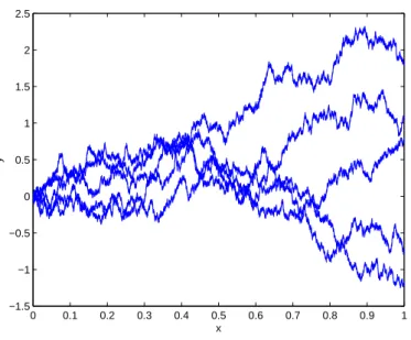
Example 2.13 (Discrete Wiener process). A discrete Wiener process can be simulated by the following Octave/Matlab code:

% Simulation of Wiener process/Brownian path

N = 1E6; % number of timesteps

randn(’state’,0); % initialize random number generator

T = 1; % final time

dt = T/(N-1); % time step

t = 0:dt:T;

dW = sqrt(dt)*randn(1,N-1); % Wiener increments

W = [0 cumsum(dW)]; % Brownian path

(19)

0 0.1 0.2 0.3 0.4 0.5 0.6 0.7 0.8 0.9 1 −1.5

−1 −0.5 0 0.5 1 1.5 2 2.5

x

y

Figure 2.2: Brownian paths

LHS = sum(t(1:N-1).*dW);

RHS = T*W(N) - sum(W(1:N-1))*dt;

Definition 2.14. A process f : [0, T]×Ω → _R is adapted if f(t,·) only depends on events which are generated byW(s),s≤t.

Remark 2.15 (Extension to adapted Itˆo integration). Itˆo integrals can be extended to adapted processes. Assume f : [0, T]×Ω→Ris adapted and that there is a constantC such that

p

E[|f(t+ ∆t, ω)−f(t, ω)|2_]_≤_C√_∆t. _(2.9)

Then the proof of Theorem2.10 shows that (2.4-2.6) still hold.

Theorem 2.16 (Basic properties of Itˆo integrals).

Suppose that f, g : [0, T]×Ω→ _R are Itˆo integrable, e.g. adapted and satifying (2.9), and that c1, c2 are constants inR. Then:

(i) RT

0 (c1f(s,·) +c2g(s,·))dW(s) =c1

RT

0 f(s,·)dW(s) +c2

RT

0 g(s,·)dW(s),

(ii) EhRT

0 f(s,·)dW(s)

i

= 0,

(iii) Eh(RT

0 f(s,·)dW(s))(

RT

0 g(s,·)dW(s))

i

=RT

(20)

Proof. To verify Property (ii), we first use thatf is adapted and the independence of the increments ∆Wn to show that for an Euler discretization

E[

N−1

X

n=0

f(tn,·)∆Wn] = N−1

X

n=0

E[f(tn,·)]E[∆Wn] = 0.

It remains to verify that the limit of Euler discretizations preserves this property: Cauchy’s inequality and the convergence result (2.6) imply that

|E[

Z T

0

f(t,·)dW(t)]|=|E[

Z T

0

f(t,·)dW(t)− N−1

X

n=0

f(tn,·)∆Wn] +

+E[

N−1

X

n=0

f(tn,·)∆Wn]|

≤ v u u tE[

Z T

0

f(t,·)dW(t)− N−1

X

n=0

f(tn,·)∆Wn !2

]→0.

Property(i)and (iii) can be verified analogously.

Example 2.17 (The Monte-Carlo method). To verify Property (ii) in Theorem 2.16 numerically for some function f we can do a Monte-Carlo simulation where

Z T

0

f(s,·)dW(s),

(21)

% Monte-Carlo simulation

N = 1E3; % number of timesteps

randn(’state’,0); % initialize random number generator

T = 1; % final time

dt = T/N; % time step

t = 0:dt:T;

M = 1E6; % number of realisations

MC = zeros(1,M); % vector to hold mean values

for i=1:M

dW = sqrt(dt)*randn(1,N); % Wiener increments

W = [0 cumsum(dW)]; % Brownian paths

f = t.^3.*sqrt(abs(W)); % some function

int = sum(f(1:N).*dW); % integral value

if i==1

MC(i) = int; else

MC(i) = (MC(i-1)*(i-1)+int)/i; % new mean value end

end

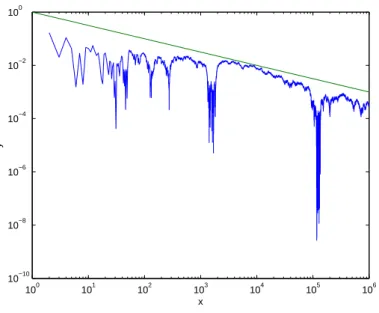
In the above code the mean value of the integral is calculated for 1, . . . , M realizations, and in Figure 2.3 we see that as the number of realizations grows, the mean value approaches zero as 1/√M. Also, from the proof of Theorem2.16it can be seen that the number of time steps does not affect this convergence, so the provided code is inefficient, but merely serves as an illustration for the general case.

Exercise 2.18. Use the forward Euler discretization to show that (a) R₀T W(s)dW(s) = 1

2W(T)

2₋_{T /2.}

(b) Property(i) and (iii) in Theorem2.16hold.

Exercise 2.19. Consider the Ornstein-Uhlenbeck process defined by

X(t) =X∞+e−at(X(0)−X∞) +b

Z t

0

e−a(t−s)dW(s), (2.10)

where X∞, a and b are given real numbers. Use the properties of the Itˆo integral to

compute E[X(t)], V ar[X(t)], limt→∞E[X(t)] and limt→∞V ar[X(t)]. Can you give an

(22)

100 101 102 103 104 105 106 10−10

10−8 10−6 10−4 10−2 100

x

y

Figure 2.3: Absolute value of the mean for different number of realizations.

Example 2.20 (Existence of a Wiener process). To construct a Wiener process on the time interval [0, T], define the Haar-functions Hi byH0(t) ≡1 and for 2n≤i <2n+1

and n= 0,1,2. . ., by

Hi(t) = 

 

 

T−1/2₂n/2 _{if (i}₋₂n₎₂−n_≤_{t/T <}_(i_{+ 0.5}₋₂n₎₂−n_, −T−1/2₂n/2 _{if (i}_{+ 0.5}₋₂n₎₂−n_≤_{t/T <}_(i_{+ 1}₋₂n₎₂−n_,

0 otherwise.

(2.11)

Then{Hi}is an orthonormal basis of L2(0, T), (why?). Define the continuous piecewise

linear function W(m)_{: [0, T}_]_→

Rby

W(m)(t) =

m X

i=1

ξiSi(t), (2.12)

where ξi, i= 1, . . . , m are independent random variables with the normal distribution

N(0,1) and

Si(t) = Z t

0

Hi(s)ds= Z T

0

1(0,t)(s)Hi(s)ds,

1₍₀_,t₎(s) =

1 ifs∈(0, t), 0 otherwise.

The functionsSi are small ”hat”-functions with a maximum value T−1/22−(n+2)/2 and

zero outside an interval of length T2−n. Let us postpone the proof that W(m) _converge

uniformly and first assume this. Then the limit W(t) =P∞

(23)

verify that the limitW is a Wiener process, we first observe thatW(t) is a sum of normal distributed variables so thatW(t) is also normal distributed. It remains to verify that the increments ∆Wn and ∆Wm are independent, for n 6= m, and E[(∆Wn)2] = ∆tn.

Parseval’s equality shows the independence and the correct variance

E[∆Wn∆Wm] =E[ X

i,j

ξiξj(Si(tn+1)−Si(tn))(Sj(tm+1)−Sj(tm))]

=X

i,j

E[ξiξj](Si(tn+1)−Si(tn))(Sj(tm+1)−Sj(tm))

=X

i

(Si(tn+1)−Si(tn))(Si(tm+1)−Si(tm))

Parseval

=

Z T

0

1₍_t_n_,t_n₊₁₎(s)1(tm,tm+1)(s)ds=

0 ifm6=n, tn+1−tn ifn=m.

To prove uniform convergence, the goal is to establish

P sup

t∈[0,T]

∞

X

i=1

|ξi|Si(t)<∞ !

= 1.

Fix a n and a t ∈[0, T] then there is only one i, satisfying 2n _≤ _{i <} ₂n+1_{, such that}

Si(t)6= 0. Denote thisiby i(t, n). Letχn≡sup2n_≤_i<₂n+1|ξ_i|, then

sup

t∈[0,T]

∞

X

i=1

|ξi|Si(t) = sup t∈[0,T]

∞

X

n=0

|ξi(t,n)|Si(t,n)(t)

≤ sup

t∈[0,T]

∞

X

n=0

|ξ_i₍_t,n₎|T−1/2₂−(n+2)/2

≤

∞

X

n=0

χnT−1/22−(n+2)/2.

If

∞

X

n=0

χn2−(n+2)/2 =∞ (2.13)

on a set with positive probability, then χn > n for infinitely many n, with positive

probability, and consequently

∞=E[

∞

X

n=0

1{χn>n}] =

∞

X

n=0

P(χn> n), (2.14)

but

P(χn> n)≤P(∪2

n+1

i=2n{|ξ_i|> n})≤2nP(|ξ₀|> n)≤C 2ne−n

2_/₄

, so that P∞

n=0P(χn> n)<∞, which contradicts (2.14) and (2.13). Therefore

P( sup

t∈[0,T]

∞

X

i=1

(24)

which proves the uniform convergence.

Exercise 2.21 (Extension to multidimensional Itˆo integrals). The multidimensional Wiener processW inRl is defined byW(t)≡(W1(t), . . . , Wl(t)), whereWi, i= 1, . . . , l are independent one-dimensional Wiener processes. Show that

I∆t≡ N−1

X

n=0

l X

i=1

fi(tn,·)∆Wni

form a Cauchy sequence withE[(I∆t1−I∆t2)

2_{] =}_O_(∆t

max), as in Theorem2.10, provided

f : [0, T]×Ω→Rl is adapted and (2.9) holds.

Exercise 2.22. Generalize Theorem2.16 to multidimensional Itˆo integrals.

Remark 2.23. A larger class of Itˆo integrable functions are the functions in the Hilbert space

V =

f : [0, T]×Ω→_Rl_{: f is adapted and} Z T

0

E[|f(t)|2_{]dt <}_∞

with the inner productR₀T E[f(t)·g(t)]dt. This follows from the fact that every function inV can be approximated by adapted functionsfh that satisfy (2.9), for some constant

C depending onh, so thatRT

0 E[|f(t,·)−fh(t,·)|

2_]dt_≤_h_as_h_→_{0. However, in contrast}

to Itˆo integration of the functions that satisfy (2.9), an approximation of the Itˆo integrals of f ∈V does not in general give a convergence rate, but only convergence.

Exercise 2.24. Read Example 2.20 and show that the Haar-functions can be used to approximate stochastic integrals RT

0 f(t)dW(t)'

Pm

i=0ξifi, for given deterministic

functions f withfi = RT

0 f(s)Hi(s)ds. In what sense doesdW(s) =

P∞

i=0ξiHids hold?

(25)

Chapter 3

Stochastic Differential Equations

This chapter extends the work on stochastic integrals, in the last chapter, and constructs approximations of stochastic differential equations with an error estimate. Existence and uniqueness is then provided by the error estimate.

We will denote byC, C0_{positive constants, not necessarily the same at each occurrence.}

3.1 Approximation and Definition of SDE

We will prove convergence of Forward Euler approximations of stochastic differential equations, following the convergence proof for Itˆo integrals. The proof is divided into four steps, including Gr¨onwall’s lemma below. The first step extends the Euler approximation

¯

X(t) to all t∈[0, T]:

Step 1. Consider a grid in the interval [0, T] defined by the set of nodes {¯_t_n}N_n¯₌₀, ¯

t0 = 0,¯t_N¯ =T and define the discrete stochastic process ¯X by the forward Euler method

¯

X(¯tn+1)−X(¯¯ tn) =a(¯tn,X(¯¯ tn))(¯tn+1−¯tn) +b(¯tn,X(¯¯ tn))(W(¯tn+1)−W(¯tn)), (3.1)

for n= 0, . . . ,N¯ −1.Now extend ¯X continuously, for theoretical purposes only, to all values of t by

¯

X(t) = ¯X(¯tn) + Z t

¯

tn

a(¯tn,X(¯¯ tn))ds+ Z t

¯

tn

b(¯tn,X(¯¯ tn))dW(s), ¯tn≤t <¯tn+1. (3.2)

In other words, the process ¯X: [0, T]×Ω→Rsatisfies the stochastic differential equation

dX(t) = ¯¯ a(t,X)dt¯ + ¯b(t,X)dW¯ (t), ¯_t_n≤t <¯_t_n₊₁_, _(3.3)

where ¯a(t,X)¯ ≡ a(¯tn,X(¯¯ tn)), ¯b(t,X)¯ ≡b(¯tn,X(¯¯ tn)),for ¯tn ≤t < ¯tn+1, and the nodal

values of the process ¯X is defined by the Euler method (3.1).

Theorem 3.1. Let X¯ and X¯¯ be forward Euler approximations of the stochastic process

X : [0, T]×Ω→_R, satisfying the stochastic differential equation

(26)

with time steps

{¯_t_n}N_n¯₌₀, ¯_t₀ _{= 0,}¯_t_¯

N =T, ¯_¯

tm

¯ ¯

N

m=0 ¯¯t0 = 0,t¯¯N¯¯ =T,

respectively, and

∆tmax= max "

max

0≤n≤_N¯−1

¯

tn+1−¯tn, max

0≤m≤_N¯¯−1

¯ ¯

tm+1−t¯¯m #

.

Suppose that there exists a positive constant C such that the initial data and the given functions a, b: [0, T]×_R→_Rsatisfy

E[|X(0)¯ |2₊_|_X(0)¯_¯ _|2_]_≤_C, _(3.5)

E[X(0)¯ −X(0)¯¯ 2]≤C∆tmax, (3.6)

and

|a(t, x)−a(t, y)|< C|x−y|,

|b(t, x)−b(t, y)|< C|x−y|, (3.7)

|a(t, x)−a(s, x)|+|b(t, x)−b(s, x)| ≤C(1 +|x|)p|t−s|. (3.8)

Then there is a constantK such that

maxnE[ ¯X2_(t,_·_{)], E[ ¯}_X_¯2_(t,_·_)]o_≤_K(T_{+ 1), t < T,} _(3.9)

and

E

¯

X(t,·)−X(t,¯¯ ·)

2

≤K∆tmax, t < T. (3.10)

The basic idea for the extension of the convergence for Itˆo integrals to stochastic differntial equations is

Lemma 3.2 (Gr¨onwall). Assume that there exist positive constantsA and K such that the function f :R→R satisfies

f(t)≤K

Z t

0

f(s)ds+A. (3.11)

Then

f(t)≤AeKt.

Proof. Let I(t)≡Rt

0 f(s)ds.Then by (3.11)

dI

(27)

and multiplying by e−Kt _{we arrive at}

d dt(Ie

−Kt₎_≤_Ae−Kt_.

After integrating, and using I(0) = 0, we obtain I ≤ A(eKt_K−1). Substituting the last result in (3.11) concludes the proof.

Proof of the Theorem. To prove (3.10), assume first that (3.9) holds. The proof is divided into the following steps:

(1) Representation of ¯X as a process in continuous time: Step 1.

(2) Use the assumptions (3.7) and (3.8).

(3) Use the property (3) from Theorem 2.16.

(4) Apply Gr¨onwall’s lemma.

Step 2. Consider another forward Euler discretization ¯X, defined on a grid with¯ nodes¯_¯

tm

¯ ¯

N

m=0, and subtract the two solutions to arrive at

¯

X(s)−X(s)¯¯ (3=.3)X(0)¯ −X(0) +¯¯

Z s

0

(¯a−¯¯a)(t)

| {z }

≡∆a(t)

dt+

Z s

0

(¯b−¯¯b)(t)

| {z }

≡∆b(t)

dW(t). (3.12)

The definition of the discretized solutions implies that

∆a(t) = (¯a−¯¯a)(t) =a(¯tn,X(¯¯ tn))−a(¯t¯m,X(¯¯¯ ¯tm)) =

= a(¯tn,X(¯¯ tn))−a(t,X(t))¯

| {z }

=(I)

+a(t,X(t))¯ −a(t,X(t))¯¯

| {z }

=(II)

+a(t,X(t))¯¯ −a(¯_t¯_m_,_X(¯¯¯ ¯_t_m₎₎

| {z }

=(III)

wheret∈[¯¯tm,t¯¯m+1)∩[¯tn,t¯n+1), as shown in Figure 3.1. The assumptions (3.7) and (3.8)

show that

|(I)| ≤ |a(¯tn,X(¯¯ tn))−a(t,X(¯¯ tn))|+|a(t,X(¯¯ tn))−a(t,X(t))¯ |

≤ C|X(¯¯ tn)−X(t)¯ |+C(1 +|X(¯¯ tn)|)|t−¯tn|1/2. (3.13)

Note that (3.7) and (3.8) imply

(28)

{tk} {¯¯_t_m}

{_t¯_n}

0

t0

¯ ¯ t0

¯ t0

T

tN

¯ ¯ t_N¯¯

¯ t_N¯

t1 t2

¯ ¯ t1

¯ t1

t3t4

¯ ¯ t2

¯ t2

t5

¯ ¯ t3

¯ t3

. . . . . . . . .

tN−2tN−1

¯ ¯ t_N¯¯₋₁

¯ t_N¯−1

Figure 3.1: Mesh points used in the proof.

Therefore

|X(¯¯ tn)−X(t)¯ |

(3.3)

= |a(¯tn,X(¯¯ tn))(t−¯tn) +b(¯tn,X(¯¯ tn))(W(t)−W(¯tn))|

(3.14)

≤ C(1 +|X(¯¯ tn)|)((t−t¯n) +|W(t)−W(¯tn)|). (3.15)

The combination of (3.13) and (3.15) shows

|(I)| ≤ C(1 +|X(¯¯ tn)|)

|W(t)−W(¯tn)|+|t−¯tn|1/2

and in a similar way,

|(III)| ≤ C(1 +|X(t)¯¯ |)|W(t)−W(¯t¯m)|+|t−¯¯tm|1/2

,

and by the assumptions (3.7)

|(II)|(3≤.7)C|X(t)¯ −X(t)¯¯ |.

Therefore, the last three inequalities imply

|∆a(t)|2 ≤ (|(I)|+|(II)|+|(III)|)2 ≤C2

|X(t)¯ −X(t)¯¯ |2

+(1 +|X(¯¯ tn)|2)(|t−t¯n|+|W(t)−W(¯tn)|2)

+ (1 +|X(¯¯¯ _t¯_m₎|2)(|t−_t¯¯_m|+|W(t)−W(¯¯tm)|2)

. (3.16)

Recall that max(t−¯_t_n_{, t}−_t¯¯_m₎≤∆tmax,and

(29)

E[|∆a(t)|2] ≤ CE[|X(t)¯ −X(t)¯¯ |2] + (1 +E[|X(¯¯ tn)|2] +E[|X(¯¯¯ t¯m)|2])∆tmax

(3.9)

≤ CE[|X(t)¯ −X(t)¯¯ |2] + ∆tmax

. (3.17)

Similarly, we have

E[|∆b(t)|2_]_≤_C_E[_|_X(t)_¯ ₋_X(t)¯_¯ _|2_{] + ∆t}

max

. (3.18)

Step 3. Define a refined grid {th}Nh=0 by the union

{th} ≡ {t¯n} ∪ ¯_¯

tm .

Observe that both the functions ∆a(t) and ∆b(t) are adapted and piecewise constant on the refined grid. The error representation (3.12) and (3) of Theorem 2.16 imply

E[|X(s)¯ −X(s)¯¯ |2] ≤ E

"

¯

X(0)−X(0) +¯¯

Z s

0

∆a(t)dt+

Z s

0

∆b(t)dW(t)

2#

≤ 3E[|X(0)¯ −X(0)¯¯ |2]

+ 3E

Z s

0

∆a(t)dt

2

+ 3E

Z s

0

∆b(t)dW(t)

2

(3.6)

≤ 3(C∆tmax+s Z s

0

E[(∆a(t))2]dt+

Z s

0

E[(∆b(t))2]dt).

(3.19)

Inequalities (3.17-3.19) combine to

E[|X(s)¯ −X(s)¯¯ |2]

(3.17−3.19)

≤ C(

Z s

0

E[|X(t)¯ −X(t)¯¯ |2]dt+ ∆tmax). (3.20)

Step 4. Finally, Gr¨onwall’s Lemma3.2applied to (3.20) implies E[|X(t)¯ −X(t)¯¯ |2]≤∆tmaxCeCt,

which finishes the proof.

Exercise 3.3. Prove (3.9). Hint: Follow Steps 1-4 and use (3.5) .

Corollary 3.4. The previous theorem yields a convergence result also in the L2 _norm

kXk2 ₌RT

0 E[X(t)

2_]dt._{The order of this convergence is}_1/2_{, i.e.} _k_X_¯₋_X¯_¯_k₌_O₍√_∆t

max).

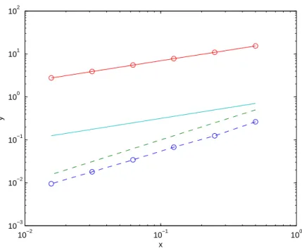
Remark 3.5(Strong and weak convergence). Depending on the application, our interest will be focused either on strong convergence

kX(T)−X(T¯ )k_L2_[Ω] =

q

(30)

or on weak convergence E[g(X(T))]−E[g( ¯X(T))], for given functions g. The next chapters will show first order convergence of expected values for the Euler method,

E[g(X(T))−g( ¯X(T))] = O(∆t),

and introduce Monte Carlo methods to approximate expected values E[g( ¯X(T))]. We will distinguish between strong and weak convergence byXn→X, denoting the strong

convergence E[|Xn−X|2]→ 0 for random variables and RT

0 E[|Xn(t)−X(t)|

2_]dt_→₀

for stochastic processes, and by Xn* X, denoting the weak convergence E[g(Xn)]→

E[g(X)] for all bounded continuous functions g.

Exercise 3.6. Show that strong convergence, Xn → X, implies weak convergence

Xn* X. Show also by an example that weak convergence, Xn * X, does not imply

strong convergence, Xn→X. Hint: Let{Xn} be a sequence of independent identically

distributed random variables.

Corollary3.4shows that successive refinements of the forward Euler approximation forms a Cauchy sequence in the Hilbert space V, defined by Definition 2.23. The limit X ∈V, of this Cauchy sequence, satisfies the stochastic equation

X(s) =X(0) +

Z s

0

a(t, X(t))dt+

Z s

0

b(t, X(t))dW(t), 0< s≤T, (3.21)

and it is unique, (why?). Hence, we have constructed existence and uniqueness of solutions of (3.21) by forward Euler approximations. Let X be the solution of (3.21). From now on we use indistinctly also the notation

dX(t) = a(t, X(t))dt+b(t, X(t))dW(t), 0< t≤T

X(0) = X0. (3.22)

These notes focus on the Euler method to approximate stochastic differential equations (3.22). The following result motivates that there is no method with higher order

convergence rate than the Euler method to control the strong errorR1

0 E[(X(t)−X(t))¯ 2_]dt,

since even for the simplest equationdX =dW any linear approximation ˆW ofW, based on N function evaluations, satisfies

Theorem 3.7. Let Wˆ(t) = f(t, W(t1), . . . , W(tN)) be any approximation of W(t),

which for fixed t is based on any linear function f(t,·) : RN → R, and a partition 0 = t0 < . . . < tN = 1 of [0,1], then the strong approximation error is bounded from

below by

Z 1

0

E[(W(t)−Wˆ(t))2]dt

1/2 ≥ √1

6N, (3.23)

(31)

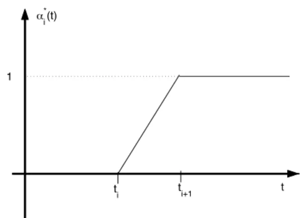
t_i t

i+1 t

!*_i(t)

1

Figure 3.2: Optimal choice for weight functions αi.

Proof. The linearity of f(t,·) implies that

ˆ W(t)≡

N X

i=1

αi(t)∆Wi

whereαi : [0,1]→R,i= 1, . . . , N are any functions. The idea is to choose the functions αi: [0,1]→R, i= 1, . . . , N in an optimal way, and see that the minimum error satisfies (3.23). We have

Z 1

0

E[(W(t)−Wˆ(t))2]dt

=

Z 1

0

E[W2(t)]−2

N X

i=1

αi(t)E[W(t)∆Wi] + N X

i,j=1

αi(t)αj(t)E[∆Wi∆Wj]

dt

=

Z 1

0

tdt−2

Z 1

0

N X

i=1

E[W(t)∆Wi]αidt+ Z 1

0

N X

i=1

α2_i(t)∆tidt

and in addition

E[W(t)∆Wi] = 

 

 

∆ti, ti+1< t

(t−ti), ti < t < ti+1

0, t < ti.

(3.24)

Perturbing the functionsαi, toαi+δi, <<1, around the minimal value of R1

0 E[

W(t)−Wˆ(t)2]dt gives the following conditions for the optimum choice of αi, cf. Figure 3.2:

−2E[W(t)∆Wi] + 2α∗i(t)∆ti = 0, i= 1, . . . , N.

(32)

min

Z 1

0

E[W(t)−Wˆ(t)]2dt=

Z 1 0 tdt− Z 1 0 N X i=1

E[W(t)∆Wi]2

∆ti

dt

=

|{z}

(3.24)

N X

n=1

(tn+ ∆tn/2)∆tn− N X

n=1

tn∆tn+ Z tn+1

tn

(t−tn)2

∆tn dt = N X n=1

(∆tn)2/6≥

1 6N.

where Exercise 3.8 is used in the last inequality and proves the lower bound of the approximation error in the theorem. Finally, we note that by (3.24) the optimal α∗_i(t) = E[W(t)∆Wi]

∆ti is infact linear interpolation of the Euler method.

Exercise 3.8. To verify the last inequality in the previous proof, compute

min

∆t N X

n=1

(∆tn)2

subject to

N X

n=1

(∆tn) = 1.

3.2 Itˆ

o’s Formula

Recall that using a forward Euler discretization we found the relation

Z T

0

W(s)dW(s) =W2_(T)/2₋_{T /2,} _or

W(s)dW(s) =d(W2(s)/2)−ds/2, (3.25) whereas in the deterministic case we have y(s)dy(s) =d(y2_(s)/2)._{The following useful}

theorem with Itˆo ’s formula generalizes (3.25) to general functions of solutions to the stochastic differential equations.

Theorem 3.9. Suppose that the assumptions in Theorem 3.1 hold and that X satisfies the stochastic differential equation

dX(s) = a(s, X(s))ds+b(s, X(s))dW(s), s >0 X(0) = X0,

and let g : (0,+∞)×_R → _R be a given bounded function in C2_((0,_∞₎_×

R). Then y(t)≡g(t, X(t)) satisfies the stochastic differential equation

dy(t) =

∂tg(t, X(t)) +a(t, X(t))∂xg(t, X(t)) +

b2_{(t, X(t))}

2 ∂xxg(t, X(t))

dt

(33)

Proof. We want to prove the Itˆo formula in the integral sense g(τ, X(τ))−g(0, X(0))

=

Z τ

0

∂tg(t, X(t)) +a(s, X(s))∂xg(t, X(t)) +

b2_{(t, X(t))}

2 ∂xxg(t, X(t))

dt

+

Z τ

0

b(t, X(t))∂xg(t, X(t))dW(t).

Let ¯X be a forward Euler approximation (3.1) and (3.2) of X, so that

∆ ¯X ≡X(t¯ n+ ∆tn)−X(t¯ n) =a(tn,X(t¯ n))∆tn+b(tn,X(t¯ n))∆Wn. (3.27)

Taylor expansion ofg up to second order gives

g(tn+ ∆tn,X(t¯ n+ ∆tn))−g(tn,X(t¯ n))

= ∂tg(tn,X(t¯ n))∆tn+∂xg(tn,X(t¯ n))∆ ¯X(tn)

+1

2∂ttg(tn,X(t¯ n))∆t

2

n+∂txg(tn,X(t¯ n))∆tn∆ ¯X(tn)

+1

2∂xxg(tn,X(t¯ n))(∆ ¯X(tn))

2₊_o(∆t2

n+|∆ ¯Xn|2). (3.28)

The combination of (3.27) and (3.28) shows

g(tm,X(t¯ m))−g(0,X(0)) =¯ m−1

X

n=0

g(tn+ ∆tn,X(t¯ n+ ∆tn))−g(tn,X(t¯ n))

=

m−1

X

n=0

∂tg∆tn+ m−1

X

n=0

(¯a∂xg∆tn+ ¯b∂xg∆Wn) +

1 2

m−1

X

n=0

(¯b)2∂xxg(∆Wn)2

+

m−1

X

n=0

(¯b∂txg+ ¯a¯b∂xxg)∆tn∆Wn+ (

1

2∂ttg+ ¯a∂txg+ 1 2¯a

2_∂

xxg)∆t2n

+

m−1

X

n=0

o(∆t2

n+|∆ ¯X(tn)|2). (3.29)

Let us first show that

m−1

X

n=0

¯_b2_∂

xxg( ¯X)(∆Wn)2 → Z t

0

b2_∂

xxg(X)ds,

as ∆tmax→0. It is sufficient to establish

Y ≡ 1

2

m−1

X

n=0

(¯b)2∂xxg((∆Wn)2−∆tn)→0, (3.30)

since (3.10) impliesPm−1

n=0(¯b)2∂xxg∆tn→

Rt

0b 2_∂

xxgds. Use the notation

(34)

E[Y2] = X

i,j

E[αiαj((∆Wi)2−∆ti)((∆Wj)2−∆tj)]

= 2X

i>j

E[αiαj((∆Wj)2−∆tj)((∆Wi)2−∆ti)] + X

i

E[α2_i((∆Wi)2−∆ti)2]

= 2X

i>j

E[αiαj((∆Wj)2−∆tj)]E[((∆Wi)2−∆ti)]

| {z }

=0

+X

i

E[α2_i]E[((∆Wi)2−∆ti)2]

| {z }

=2∆t2

i

→0,

when ∆tmax →0, therefore (3.30) holds. Similar analysis with the other terms in (3.29)

concludes the proof.

Remark 3.10. The preceding result can be remembered intuitively by a Taylor expansion of g up to second order

dg =∂tg dt+∂xg dX+

1

2∂xxg (dX)

2

and the relations: dtdt=dtdW =dW dt= 0 and dW dW =dt.

Example 3.11. LetX(t) =W(t) andg(x) = x₂2.Then

d

W2_(s)

2

=W(s)dW(s) + 1/2(dW(s))2=W(s)dW(s) +ds/2.

Exercise 3.12. LetX(t) =W(t) andg(x) =x4_._{Verify that}

d(W4_{(s)) = 6W}2_(s)ds_{+ 4W}3_(s)dW_(s)

and

d

ds(E[g(W(s))]) = d

ds(E[(W(s))

4_{]) = 6s.}

Apply the last result to computeE[W4_{(t)] and}_E[(W2_(t)₋_t)2_].

Exercise 3.13. Generalize the previous exercise to deteremine E[W2n_(t)].

Example 3.14. We want to computeRT

0 tdW(t).Takeg(t, x) =tx,and againX(t) =

W(t),so that

tW(t) =

Z t

0

sdW(s) +

Z t

0

W(s)ds

and finally Rt

0 sdW(s) =tW(t)−

Rt

(35)

Exercise 3.15. Consider the stochastic differential equation dX(t) =−a(X(t)−X∞)dt+bdW(t),

with initial dataX(0) =X0∈Rand givena, b∈R.

(i) Using that

X(t)−X(0) =−a

Z t

0

(X(s)−X∞)dt+bW(t),

take the expected value and find an ordinary differential equation for the function m(t)≡E[X(t)].

(ii) Use Itˆo ’s formula to find the differential of (X(t))2 _{and apply similar ideas as in}

(i) to computeV ar[X(t)].

(iii) Use an integrating factor to derive the exact solution (2.10) in Example 2.19. Compare your results from(i) and (ii)with this exact solution.

Example 3.16. Consider the stochastic differential equation dS(t) =rS(t)dt+σS(t)dW(t),

used to model the evolution of stock values. The values of r (interest rate) and σ (volatility) are assumed to be constant. Our objective is to find a closed expression for the solution, often called geometric Brownian motion. Letg(x) = ln(x). Then a direct application of Itˆo formula shows

dln(S(t)) =dS(t)/S(t)−1/2

σ2_S2_(t)

S2_(t)

dt=rdt−σ

2

2 dt+σdW(t), so that

ln

S(T) S(0)

=rT −T σ

2

2 +σW(T) and consequently

S(T) =e(r−σ

2

2 )T+σW(T)S(0). (3.31)

(36)

% Stong and weak convergence for the Euler method

steps = [1:6]; for i=steps

N = 2^i % number of timesteps

randn(’state’,0);

T = 1; dt = T/N; t = 0:dt:T; r = 0.1; sigma = 0.5; S0 = 100;

M = 1E6; % number of realisations

S = S0*ones(M,1); % S(0) for all realizations

W = zeros(M,1); % W(0) for all realizations

for j=1:N

dW = sqrt(dt)*randn(M,1); % Wiener increments

S = S + S.*(r*dt+sigma*dW); % processes at next time step

W = W + dW; % Brownian paths at next step

end

ST = S0*exp( (r-sigma^2/2)*T + sigma*W ); % exact final value

wError(i) = mean(S-ST)); % weak error

sError(i) = sqrt(mean((S-ST).^2)); % strong error

end

dt = T./2^steps;

loglog(dt,abs(wError),’o--’,dt,dt,’--’,dt,abs(sError),’o-’,dt,sqrt(dt))

Exercise 3.18. Suppose that we want to simulateS(t), defined in the previous example by means of the forward Euler method, i.e.

Sn+1= (1 +r∆tn+σ∆Wn)Sn, n= 0, . . . , N

As with the exact solutionS(t), we would like to haveSnpositive. Then we could choose

the time step ∆tn to reduce the probability of hitting zero

P(Sn+1<0|Sn=s)< 1. (3.32)

Motivate a choice for and find then the largest ∆tn satisfying (3.32).

Remark 3.19. The Wiener process has unbounded variation i.e.

E

Z T

0

|dW(s)|

= +∞.

(37)

10−2 10−1 100 10−3

10−2 10−1 100 101 102

x

y

Figure 3.3: Strong and weak convergence.

We have for a uniform mesh ∆t=T /N

E[

N−1

X

i=0

|∆Wi|] = N−1

X

i=0

E[|∆Wi|] = N−1

X

i=0

r

2∆ti

π

=

r

2T π

N−1

X

i=0

p

1/N =

r

2N T

π → ∞, asN → ∞.

3.3 Stratonovich Integrals

Recall from Chapter 2 that Itˆo integrals are constructed via forward Euler discretizations and Stratonovich integrals via the trapezoidal method, see Exercise 3.20. Our goal here is to express a Stratonovich integral

Z T

0

g(t, X(t))◦dW(t)

in terms of an Itˆo integral. Assume then thatX(t) satisfies the Itˆo differential equation

(38)

Then the relation reads

Z T

0

g(t, X(t))◦dW(t) =

Z T

0

g(t, X(t))dW(t)

+ 1 2

Z T

0

∂xg(t, X(t))b(t, X(t))dt. (3.33)

Therefore, Stratonovich integrals satisfy

dg(t, X(t)) =∂tg(t, X(t))dt+∂xg(t, X(t))◦dX(t), (3.34)

just like in the usual calculus.

Exercise 3.20. Use that Stratonovich integralsg(t, X(t))◦dW(t) are defined by limits of the trapezoidal method to verify (3.33), cf. Remark2.9.

Exercise 3.21. Verify the relation (3.34), and use this to show that dS(t) =rS(t)dt+ σS(t)◦dW(t) impliesS(t) =ert+σW(t)_S(0).

Remark 3.22 (Stratonovich as limit of piecewise linear interpolations). LetRN_(t) _≡

W(tn) +W(tn_t_n+1₊₁)−₋W_t_n(tn)(t−tn), t∈(tn, tn+1) be a piecewise linear interpolation ofW on a

given grid, and define XN _by_dXN_{(t) =}_a(XN_(t))dt₊_b(XN_(t))dRN_{(t). Then} _XN _→_X

inL2_{, where}_X _{is the solution of the Stratonovich stochastic differential equation}

dX(t) =a(X(t))dt+b(X(t))◦dW(t). In the special case whena(x) =rx and b(x) =σx this follows from

d(ln(XN(t))) =rdt+σdRN, so that

XN(t) =ert+σRN(t)X(0).

The limitN → ∞ impliesXN_(t)_→_{X(t) =}_ert+σW(t)_{X(0), as in Exercise} _3.21.

3.4 Systems of SDE

Let W1, W2, . . . , Wl be scalar independent Wiener processes. Consider thel-dimensional

Wiener process W = (W1, W2, . . . , Wl) andX: [0, T]×Ω→Rd satisfying for given drift a: [0, T]×Rd→ Rd and diffusion b: [0, T]×Rd→Rd×l the Itˆo stochastic differential equation

dXi(t) =ai(t, X(t))dt+bij(t, X(t))dWj(t), f or i= 1. . . d. (3.35)

Here and below we use of the summation convention

αjβj ≡ X

j

αjβj,

(39)

Theorem 3.23 (Itˆo ’s formula for systems). Let

dXi(t) =ai(t, X(t))dt+bij(t, X(t))dWj(t), f or i= 1. . . d,

and consider a smooth and bounded function g:R+×Rd→R.Then

dg(t, X(t)) =

∂tg(t, X(t)) +∂xig(t, X(t))ai(t, X(t))

+1

2bik(t, X(t))∂xixjg(t, X(t))bjk(t, X(t))

dt

+∂xig(t, X(t))bij(t, X(t))dWj(t),

or in matrix vector notation

dg(t, X(t)) =

∂tg(t, X(t)) +∇xg(t, X(t)) a(t, X(t))

+1

2trace b(t,X(t))b

T_(t,_X(t))_∇2

xg(t,X(t))

dt

+∇_xg(t, X(t))b(t, X(t))dW(t).

Remark 3.24. The formal rules to remember Theorem 3.23are Taylor expansion to second order and

dWjdt = dtdt= 0

dWidWj = δijdt=

dt if i=j,

0 otherwise. (3.36)

(40)

Chapter 4

The Feynman-Kˇ

ac Formula and

the Black-Scholes Equation

4.1 The Feynman-Kˇ

ac Formula

Theorem 4.1. Suppose thata, bandgare differentiable to any order and these derivatives are bounded. Let X be the solution of the stochastic differential equation,

dX(t) =a(t, X(t))dt+b(t, X(t))dW(t),

and let u(x, t) = E[g(X(T))|X(t) = x]. Then u is the solution of the Kolmogorov backward equation

L∗u ≡ ut + aux +

1 2b

2_u

xx = 0, t < T (4.1)

u(x, T) = g(x).

Proof. Define ˆu to be the solution of (4.1), i.e. L∗_u_ˆ _{= 0,}_u(_ˆ _·_{, T}_{) =} _g(_·_{). We want to}

verify that ˆuis the expected value E[g(X(T))|X(t) =x]. The Itˆo formula applied to ˆ

u(X(t), t) shows

dˆu(X(t), t) =

ˆ

ut + aˆux +

1 2b

2_u_ˆ

xx

dt + bˆuxdW

= L∗udtˆ + bˆuxdW.

Integrate this from ttoT and useL∗uˆ = 0 to obtain ˆ

u(X(T), T) − u(X(t), t)ˆ = g(X(T)) − u(X(t), t)ˆ

=

Z T

t

bˆuxdW(s).

Take the expectation and use that the expected value of the Itˆo integral is zero,

E[g(X(T))|X(t) =x]−u(x, t)ˆ = E[

Z T

t

b(s, X(s))ˆux(X(s), s)dW(s)|X(t) =x]

(41)

Therefore

ˆ

u(x, t) = E[g(X(T))|X(t) =x],

which proves the theorem since the solution of Equation (4.1) is unique.

Exercise 4.2 (Maximum Principle). Let the function u satisfy

ut + aux +

1 2b

2_u

xx = 0, t < T

u(x, T) = g(x).

Prove that u satisfies the maximum principle

max

0<t<T, x∈_Ru(t, x)≤maxx∈_R g(x).

4.2 Black-Scholes Equation

Example 4.3. Let f(t, S(t)) be the price of a European put option whereS(t) is the price of a stock satisfying the stochastic differential equationdS=µSdt+σSdW, where the volatilityσ and the driftµ are constants. Assume also the existence of a risk free paper,B, which follows dB=rBdt, where r, the risk free rent is a constant. Find the partial differential equation of the price, f(t, S(t)), of an option.

Solution. Consider the portfolioI =−f+α S+βB forα(t), β(t)∈R. Then the Itˆo formula and self financing, i.e. dI=−df+αdS+βdB, imply

dI = −df + αdS + βdB = −(ft + µSfS +

1 2σ

2_S2_f

SS)dt − fSσSdW +α(µSdt+σSdW) +βrBdt

=

−(ft + µSfS +

1 2σ

2_S2_f

SS) + (αµS + βrB)

dt + (−fS + α)σSdW.

Now chooseα such that the portfolioI becomes riskless, i.e. α = fS, so that

dI =

−(ft + µSfS +

1 2σ

2_S2_f

SS) + (fSµS + βrB)

dt

=

−(ft +

1 2σ

2_S2_f

SS) + βrB

dt. (4.2)

Assume also that the existence of an arbitrage opportunity is precluded, i.e. dI =rIdt, wherer is the interest rate for riskless investments, to obtain

dI = r(−f + αS+βB)dt

(42)

Equation (4.2) and (4.3) show that

ft + rsfs +

1 2σ

2_s2_f

ss=rf, t < T, (4.4)

and finally at the maturity time T the contract value is given by definition, e.g. a standard European put option satisfies for a given exercise price K

f(T, s) = max(K−s,0).

The deterministic partial differential equation (4.4) is called the Black-Scholes equation. The existence of adaptedβ is shown in the exercise below.

Exercise 4.4(Replicating portfolio). It is said that the self financing portfolio,αS+βB, replicates the option f. Show that there exists an adapted stochastic process β(t), satisfying self financing,d(αS+βB) =αdS+βdB, withα =fS.