Document Image Analysis
Lawrence O’Gorman
Rangachar Kasturi
ISBN 0-8186-7802-X
Library of Congress Number 97-17283
1997
This book is now out of print
2009
We have recreated this online document from the authors’ original files
This version is formatted differently from the published book; for example,
the references in this document are included at the end of each section instead
of at the end of each chapter. There are also minor changes in content.
Table of Contents
Preface
Chapter 1
What is a Document Image and What Do We Do With It?
Chapter 2
Preparing the Document Image
2.1: Introduction... 8
2.2: Thresholding ... 9
2.3: Noise Reduction... 19
2.4: Thinning and Distance Transform ... 25
2.5: Chain Coding and Vectorization... 34
2.6: Binary Region Detection ... 39
Chapter 3
Finding Appropriate Features
3.1: Introduction... 443.2: Polygonalization ... 45
3.3: Critical Point Detection ... 52
3.4: Line and Curve Fitting ... 59
3.5: Shape Description and Recognition... 67
Chapter 4
Recognizing Components of Text Documents
4.1: Introduction... 734.2: Skew Estimation ... 75
4.3: Layout Analysis ... 82
4.4: Machine-Printed Character Recognition ... 93
4.5: Handwritten Character Recognition ... 99
4.6: Document and Forms Processing Systems ... 101
4.7: Commercial State and Future Trends ... 104
Chapter 5
Recognizing Components of Graphics Documents
5.1: Introduction... 1085.2: Extraction of Lines and Regions... 111
5.3: Graphics Recognition and Interpretation ... 114
Preface
In the late 1980’s, the prevalence of fast computers, large computer memory, and inexpensive
scanners fostered an increasing interest in document image analysis. With many paper documents
being sent and received via fax machines and being stored digitally in large document databases,
the interest grew to do more with these images than simply view and print them. Just as humans
extract information from these images, research was performed and commercial systems built to
read text on a page, to find fields on a form, and to locate lines and symbols on a diagram. Today,
the results of research work in document processing and optical character recognition (OCR) can
be seen and felt every day. OCR is used by the post offices to automatically route mail.
Engineer-ing diagrams are extracted from paper for computer storage and modification. Handheld
comput-ers recognize symbols and handwriting for use in niche markets such as inventory control. In the
future, applications such as these will be improved, and other document applications will be
added. For instance, the millions of old paper volumes now in libraries will be replaced by
com-puter files of page images that can be searched for content and accessed by many people at the
same time — and will never be mis-shelved. Business people will carry their file cabinets in their
portable computers, and paper copies of new product literature, receipts, or other random notes
will be instantly filed and accessed in the computer. Signatures will be analyzed by the computer
for verification and security access.
This book describes some of the technical methods and systems used for document processing of
text and graphics images. The methods have grown out of the fields of digital signal processing,
digital image processing, and pattern recognition. The objective is to give the reader an
under-standing of what approaches are used for application to documents and how these methods apply
to different situations. Since the field of document processing is relatively new, it is also dynamic,
so current methods have room for improvement, and innovations are still being made. In addition,
there are rarely definitive techniques for all cases of a certain problem.
The intended audience is executives, managers, and other decision makers whose business
requires some acquaintance or understanding of document processing. (We call this group
“exec-utives” in accordance with the Executive Briefingseries.) Some rudimentary knowledge of com-puters and computer images will be helpful background for these readers. We begin at basic
as to have knowledge of picture processing as to have a level of comfort with the tasks that can be
accomplished on a computer and the digital nature by which any computer technique operates. A
grasp of the terminology goes a long way toward aiding the executive in discussing the problem.
For this reason, each section begins with a list of keywords that also appears in the index. With
knowledge of the terminology and whatever depth of method or system understanding that he or
she decides to take from the text, the executive should be well-equipped to deal with document
processing issues.
In each chapter, we attempt to identify major problem areas and to describe more than one method
applied to each problem, along with advantages and disadvantages of each method. This gives an
understanding of the problems and also the nature of trade-offs that so often must be made in
choosing a method. With this understanding of the problem and a knowledge of the methodology
options, an executive will have the technical background and context with which to ask questions,
judge recommendations, weigh options, and make decisions.
We include both technology description as well as references to the technical papers that best give
details on the techniques. The technology descriptions in the book are enough to understand the
methods; if implementation is desired, the references will facilitate this. Popular and accepted
methods are emphasized so that the executive can compare against the options offered against the
accepted options. In many cases, these options are advanced methods not currently used in
com-mercial products. But, depending on the level of need, advanced methods can be implemented by
the programming staff to yield better results. We also describe many full systems entailing
docu-ment processing. These are described from a high enough level as to be generally understandable
and, in addition, to motivate understanding of some of the techniques.
The book is organized in the sequence that document images are usually processed. After
docu-ment input by digital scanning, pixel processing is first performed. This level of processing
includes operations that are applied to all image pixels. These include noise removal, image
enhancement, and segmentation of image components into text and graphics (lines and symbols).
Feature-level analysis treats groups of pixels as entities, and includes line and curve detection, and
shape description. The last two chapters separate text and graphics analysis. Text analysis
includes optical character recognition (OCR) and page format recognition. Graphics analysis
Chapter 1
What is a Document Image and What Do We Do With It?
Traditionally, transmission and storage of information have been by paper documents. In the past
few decades, documents increasingly originate on the computer, however, in spite of this, it is
unclear whether the computer has decreased or increased the amount of paper. Documents are still
printed out for reading, dissemination, and markup. The oft-repeated cry of the early 1980's for
the “paper-less office” has now given way to a different objective, dealing with the flow of
elec-tronic and paper documents in an efficient and integrated way. The ultimate solution would be for
computers to deal with paper documents as they deal with other forms of computer media. That is,
paper would be as readable by the computer as magnetic and optical disks are now. If this were
the case, then the major difference — and the major advantage — would be that, unlike current
computer media, paper documents could be read by both the computer and people.
The objective of document image analysis is to recognize the text and graphics components in
images, and to extract the intended information as a human would. Two categories of document
image analysis can be defined (see Figure 1). Textual processing deals with the text components
of a document image. Some tasks here are: recognizing the text by optical character recognition
(OCR), determining the skew (any tilt at which the document may have been scanned into the
computer), finding columns, paragraphs, text lines, and words. Graphics processing deals with the
non-textual line and symbol components that make up line diagrams, delimiting straight lines
between text sections, company logos, etc. Because many of these graphics components consist of
lines, such processing includes line thinning, line fitting, and corner and curve detection. (It
should be noted that the use of “line” in this book can mean straight, curved, or piecewise straight
and/or curved lines. When straightness or curvedness is important, it will be specified.) Pictures
are a third major component of documents, but except for recognizing their location on a page,
further analysis of these is usually the task of other image processing and machine vision
tech-niques, so we do not deal with picture processing in this book. After application of these text and
graphics analysis techniques, the megabytes of initial data are culled to yield a much more concise
semantic description of the document.
to see the stacks of paper. Some may be computer generated, but if so, inevitably by different
computers and software such that even their electronic formats are incompatible. Some will
include both formatted text and tables as well as handwritten entries. There are different sizes,
from a 3.5x2" (8.89x5.08cm) business card to a 34x44" (86x111cm) engineering drawing. In
many businesses today, imaging systems are being used to store images of pages to make storage
and retrieval more efficient. Future document analysis systems will recognize types of documents,
enable the extraction of their functional parts, and be able to translate from one computer
gener-ated format to another. There are many other examples of the use of and need for document
sys-tems. Glance behind the counter in a post office at the mounds of letters and packages. In some
U.S. post offices, over a million pieces of mail must be handled each day. Machines to perform
sorting and address recognition have been used for several decades, but there is the need to
pro-cess more mail, more quickly, and more accurately. As a final example, examine the stacks of a
library, where row after row of paper documents are stored. Loss of material, misfiling, limited
numbers of each copy, and even degradation of materials are common problems, and may be Document Processing
Textual Processing Graphical Processing
Optical Character Recognition
Page Layout Analysis
Line Processing Region and
Symbol Processing
Figure 1. A hierarchy of document processing subareas listing the types of document
components dealt with in each subarea. Text Skew, text lines,
text blocks, and paragraphs
Straight lines, corners and curves
improved by document analysis techniques. All of these examples serve as applications ripe for
the potential solutions of document image analysis.
Though document image analysis has been in use for a couple of decades (especially in the
bank-ing business for computer readbank-ing of numeric check codes), it is just in the late 1980’s and early
1990’s that the area has grown much more rapidly. The predominant reason for this is greater
speed and lower cost of hardware now available. Since fax machines have become ubiquitous, the
cost of optical scanners for document input have dropped to the level that these are affordable to
even small businesses and individuals. Though document images contain a relatively large
amount of data, even personal computers now have adequate speed to process them. Computer
main memory also is now adequate for large document images, but more importantly, optical
memory is now available for mass storage of large amounts of data. This improvement in
hard-ware, and the increasing use of computers for storing paper documents, has led to increasing
interest in improving the technology of document processing and recognition. An essential
com-plement to these hardware improvements are the advancements being made in document analysis
software and algorithms. With OCR recognition rates now in the mid to high 90% range, and
other document processing methods achieving similar improvements, these advances in research
have also driven document image analysis forward.
As these improvements continue, document systems will become increasingly more evident in the
form of every-day document systems. For instance, OCR systems will be more widely used to
store, search, and excerpt from paper-based documents. Page layout analysis techniques will
rec-ognize a particular form, or page format and allow its duplication. Diagrams will be entered from
pictures or by hand, and logically edited. Pen-based computers will translate handwritten entries
into electronic documents. Archives of paper documents in libraries and engineering companies
will be electronically converted for more efficient storage and instant delivery to a home or office
computer. Though it will be increasingly the case that documents are produced and reside on a
computer, the fact that there are very many different systems and protocols, and also the fact that
paper is a very comfortable medium for us to deal with, ensures that paper documents will be with
us to some degree for many decades to come. The difference will be that they will finally be
Hardware Advancements and the Evolution of Document Image Analysis
The field of document image analysis can be traced back through a computer lineage that includes
digital signal processing and digital image processing. Digital signal processing, whose study and
use was initially fostered by the introduction of fast computers and algorithms such as the fast
Fourier transform in the mid 1960's, has as its objective the interpretation of one-dimensional
sig-nals such as speech and other audio. In the early 1970's, with larger computer memories and still
faster processors, image processing methods and systems were developed for analysis of
two-dimensional signals including digitized pictures. Special fields of image processing are associated
with particular application — for example, biomedical image processing for medical images,
machine vision for processing of pictures in industrial manufacturing, and computer vision for
processing images of three-dimensional scenes used in robotics, for example.
In the mid- to late-1980's, document image analysis began to grow rapidly. Again, this was
pre-dominantly due to hardware advancements enabling processing to be performed at a reasonable
cost and time. Whereas a speech signal is typically processed in frames of 256 samples long and a
machine vision image size is 512x512 pixels, a document image is from 2550x3300 pixels for a
business letter digitized at 300 dots per inch (dpi) (12 dots per millimeter) to 34000x44000 pixels
for a 34x44" E-sized engineering diagram digitized at 1000 dpi.
Commercial document analysis systems are now available for storing business forms, performing
OCR on typewritten text, and compressing engineering drawings. Document analysis research
continues to pursue more intelligent handling of documents, better compression — especially
through component recognition — and faster processing.
From Pixels to Paragraphs and Drawings
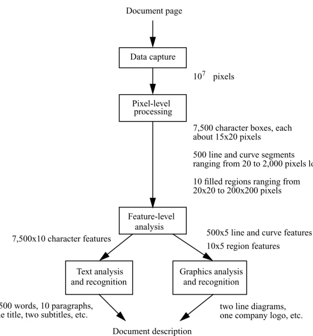
Figure 2 illustrates a common sequence of steps in document image analysis. This is also the
organization of chapters in this book. After data capture, the image undergoes pixel level
process-ing and feature analysis, then text and graphics are treated separately for recognition of each.
Data capture is performed on a paper document usually by optical scanning. The resulting data is
stored in a file of picture elements, called pixels, that are sampled in a grid pattern throughout the
document. These pixels may have values: OFF (0) or ON (1) for binary images, 0-255 for
resolu-tion of 300 dpi, a 8.5x11'' page would yield an image of 2550x3300 pixels. It is important to
understand that the image of the document contains only raw data that must be further analyzed to
glean the information. For instance, Figure 3shows the image of a letter “e”. This is a pixel array
of ON or OFF values whose shape is known to humans as the letter “e” — however to a computer
it is just a string of bits in computer memory.
Pixel-level processing (Chapter 2). This stage includes binarization, noise reduction, signal Document page
Pixel-level processing
Feature-level analysis Data capture
Text analysis and recognition
Graphics analysis and recognition
Document description
107 pixels
7,500 character boxes, each about 15x20 pixels
500 line and curve segments
ranging from 20 to 2,000 pixels long
10 filled regions ranging from 20x20 to 200x200 pixels
500x5 line and curve features
10x5 region features 7,500x10 character features
two line diagrams, one company logo, etc. 1,500 words, 10 paragraphs,
one title, two subtitles, etc.
Figure 2. A typical sequence of steps for document analysis, along with examples of
enhancement, and segmentation. For gray-scale images with information that is inherently binary
such as text or graphics, binarization is usually performed first. The objective in methods for
bina-rization is to automatically choose a threshold that separates the foreground and background
information. An example that has seen much research is the extraction of handwriting from a bank
check — especially a bank check containing a scenic image as a background.
Document image noise occurs from image transmission, photocopying, or degradation due to
aging. Salt-and-pepper noise (also called impulse noise, speckle noise, or just dirt) is a common
form of noise on a binary image. It consists of randomly distributed black specks on white
back-ground and white specks on black backback-ground. It is reduced by performing filtering on the image
where the background is “grown'' into the noise specks, thus filling these holes. Signal
enhance-ment is similar to noise reduction, but uses domain knowledge to reconstitute expected parts of
the signal that have been lost. Signal enhancement often applied to graphics components of
docu-ment images to fill gaps in lines that are known to be continuous otherwise.
Figure 3. A binary image of the letter “e” is made up of ON and OFF pixels,
Segmentation occurs on two levels. On the first level, if the document contains both text and
graphics, these are separated for subsequent processing by different methods. On the second level,
segmentation is performed on text by locating columns, paragraphs, words, titles, and captions;
and on graphics, segmentation usually includes separating symbol and line components. For
instance, in a page containing a flow chart with an accompanying caption, text and graphics are
first separated. Then the text is separated into that of the caption and that of the chart. The
graph-ics is separated into rectangles, circles, connecting lines, etc.
Feature-level analysis (Chapter 3).In a text image, the global features describe each page, and
consist of skew (the tilt at which the page has been scanned), line lengths, line spacing, etc. There
are also local features of individual characters, such as font size, number of loops in a character,
number of crossings, accompanying dots, etc., which are used for OCR.
In a graphical image, global features describe the skew of the page, the line widths, range of
cur-vature, minimum line lengths, etc. Local features describe each corner, curve, and straight line, as
well as the rectangles, circles, and other geometric shapes.
Recognition of text and graphics (Chapters 4 and 5). The final step is the recognition and
description step, where components are assigned a semantic label and the entire document is
described as a whole. It is at this stage that domain knowledge is used most extensively. The result
is a description of a document as a human would give it. For a text image, we refer not to pixel
groups, or blobs of black on white, but to titles, subtitles, bodies of text, footnotes, etc. Depending
on the arrangement of these text blocks, a page of text may be a title page of a paper, a table of
contents of a journal, a business form, or the face of a mail piece. For a graphical image, an
elec-trical circuit diagram for instance, we refer not to lines joining circles and triangles and other
shapes, but to connections between AND gates, transistors and other electronic components. The
components and their connections describe a particular circuit that has a purpose in the known
domain. It is this semantic description that is most efficiently stored and most effectively used for
Chapter 2
Preparing the Document Image
2.1: Introduction
Data capture of documents by optical scanning or by digital video yields a file of picture
ele-ments, or pixels, that is the raw input to document analysis. These pixels are samples of intensity
values taken in a grid pattern over the document page, where the intensity values may be: OFF (0)
or ON (1) for binary images, 0-255 for gray-scale images, and 3channels of 0-255 color values
for color images. The first step in document analysis is to perform processing on this image to
prepare it for further analysis. Such processing includes: thresholding to reduce a gray-scale or
color image to a binary image, reduction of noise to reduce extraneous data, and thinning and
region detection to enable easier subsequent detection of pertinent features and objects of interest.
This pixel-level processing (also called preprocessing and low-level processing in other literature)
2.2: Thresholding
Keywords: thresholding, binarization, global thresholding, adaptive thresholding, intensity histogram
In this treatment of document processing, we deal with images containing text and graphics of
binary information. That is, these images contain a single foreground level that is the text and
graphics of interest, and a single background level upon which the foreground contrasts. We will
also call the foreground: objects, regions of interest, or components. (Of course, documents may
also contain true gray-scale (or color) information, such as in photographic figures; however,
besides recognizing the presence of a gray-scale picture in a document, we leave the analysis of
pictures to the more general fields of image analysis and machine vision.) Though the information
is binary, the data — in the form of pixels with intensity values — are not likely to have only two
levels, but instead a range of intensities. This may be due to nonuniform printing or nonuniform
reflectance from the page, or a result of intensity transitions at the region edges that are located
between foreground and background regions. The objective in binarization is to mark pixels that
belong to true foreground regions with a single intensity (ON) and background regions with a
dif-ferent intensity (OFF). Figure 1 illustrates the results of binarizing a document image at difdif-ferent
threshold values. The ON-values are shown in black in our figures, and the OFF-values are white.
For documents with a good contrast of components against a uniform background, binary
scan-ners are available that combine digitization with thresholding to yield binary data. However, for
the many documents that have a wide range of background and object intensities, this fixed
threshold level often does not yield images with clear separation between the foreground
compo-nents and background. For instance, when a document is printed on differently colored paper or
when the foreground components are faded due to photocopying, or when different scanners have
different light levels, the best threshold value will also be different. For these cases, there are two
alternatives. One is to empirically determine the best binarization setting on the scanner (most
binary scanners provide this adjustment), and to do this each time an image is poorly binarized.
The other alternative is to start with gray-scale images (having a range of intensities, usually from
0 to 255) from the digitization stage, then use methods for automatic threshold determination to
better perform binarization. While the latter alternative requires more input data and processing,
a) histogram
b) low threshold
d) high threshold c) good threshold
Figure 1. Image binarization. a) Histogram of original gray-scale image. Horizontal
axis shows markings for threshold values of images below. The lower peak
is for the white background pixels, and the upper peak is for the black
fore-ground pixels. Image binarized with: (b) too low a threshold value, c) a good
threshold value, and d) too high a threshold value. (c)
(b) (d)
255 (black) intensity value 0
good images, and precluding the need for time-consuming manual adjustment and repeated
digiti-zation. The following discussion presumes initial digitization to gray-scale images.
If the pixel values of the components and those of the background are fairly consistent in their
respective values over the entire image, then a single threshold value can be found for the image.
This use of a single threshold for all image pixels is called global thresholding. Processing
meth-ods are described below that automatically determine the best global threshold value for different
images. For many documents, however, a single global threshold value cannot be used even for a
single image due to nonuniformities within foreground and background regions. For example, for
a document containing white background areas as well as highlighted areas of a different
back-ground color, the best thresholds will change by area. For this type of image, different threshold
values are required for different local areas; this is adaptive thresholding, and is also described
below.
2.2.1: Global Thresholding
The most straightforward way to automatically select a global threshold is by use of a histogram
of the pixel intensities in the image. The intensity histogram plots the number of pixels with
val-ues at each intensity level. See Figure1 for a histogram of a document image. For an image with
well-differentiated foreground and background intensities, the histogram will have two distinct
peaks. The valley between these peaks can be found as the minimum between two maxima and
the intensity value there is chosen as the threshold that best separates the two peaks.
There are a number of drawbacks to global threshold selection based on the shape of the intensity
distribution. The first is that images do not always contain well-differentiated foreground and
background intensities due to poor contrast and noise. A second is that, especially for an image of
sparse foreground components, such as for most graphics images, the peak representing the
fore-ground will be much smaller than the peak of the backfore-ground intensities. This often makes it
dif-ficult to find the valley between the two peaks. In addition, reliable peak and valley detection are
separate problems unto themselves. One way to improve this approach is to compile a histogram
of pixel intensities that are weighted by the inverse of their edge strength values [Mason 1975].
Region pixels with low edge values will be weighted more highly than boundary and noise pixels
with higher edge values, thus sharpening the histogram peaks due to these regions and facilitating
pix-els with high edge values, then choose the threshold at the peak of this histogram, corresponding
to the transition between regions [Weszka 1979]. This requires peak detection of a single
maxi-mum, and this is often easier than valley detection between two peaks. This approach also reduces
the problem of large size discrepancy between foreground and background region peaks because
edge pixels are accumulated on the histogram instead of region pixels; the difference between a
small and large size area is a linear quantity for edges versus a much larger squared quantity for
regions. A third method uses a Laplacian weighting. The Laplacian is the second derivative
oper-ator, which highly weights transitions from regions into edges (the first derivative highly weights
edges). This will highly weight the border pixels of both foreground regions and their surrounding
backgrounds, and because of this the histogram will have two peaks of similar area. Though these
histogram shape techniques offer the advantage that peak and valley detection are intuitive, still
peak detection is susceptible to error due to noise and poorly separated regions. Furthermore,
when the foreground or background region consists of many narrow regions, such as for text, edge
and Laplacian measurement may be poor due to very abrupt transitions (narrow edges) between
foreground and background.
A number of techniques determine classes by formal pattern recognition techniques that optimize
some measure of separation. One approach is minimum error thresholding [Kittler 1986, Ye
1988]. (See Figure 2.) Here, the foreground and background intensity distributions are modeled as
normal (Gaussian or bell-shaped) probability density functions. For each intensity value (from 0
to 255, or a smaller range if the threshold is known to be limited to it), the means and variances
are calculated for the foreground and background classes, and the threshold is chosen such that
the misclassification error between the two classes is minimized. This latter method is classified
as a parametric technique because of the assumption that the gray-scale distribution can be
mod-eled as a probability density function. This is a popular method for many computer vision
applica-tions, but some experiments indicate that documents do not adhere well to this model, and thus
results with this method are poorer than parametric approaches [Abutaleb 1989]. One
non-parametric approach is Otsu’s method [Otsu 1979, Reddi 1984]. Calculations are first made of the
ratio of between-class variance to within-class variance for each potential threshold value. The
classes here are the foreground and background pixels and the purpose is to find the threshold that
maximizes the variance of intensities between the two classes, and minimizes them within each
maximum is the chosen threshold. A similar approach to Otsu’s employs an information theory
measure, entropy, which is a measure of the information in the image expressed as the average
number of bits required to represent the information [Kapur 1985, Abutaleb 1989]. Here, the
entropy for the two classes is calculated for each potential threshold, and the threshold where the
sum of the two entropies is largest is chosen as the best threshold. Another thresholding approach
is by moment preservation [Tsai 1986]. This is less popular than the methods above, however, we
have found it to be more effective in binarizing document images containing text. For this method,
a threshold is chosen that best preserves moment statistics in the resulting binary image as
com-pared with the initial gray-scale image. These moments are calculated from the intensity
histo-gram — the first four moments are required for binarization.
Many images have more than just two levels. For instance, magazines often employ boxes to
highlight text where the background of the box has a different color than the white background of intensity intensity
background peak
foreground peak
area of misclassification error
Figure 2. Illustration of misclassification error in thresholding. On left is intensity
histogram showing foreground and background peaks. On right, the tails
of the foreground and background populations have been extended to
show the intensity overlap of the two populations. It is evident that this
overlap makes it impossible to correctly classify all pixels by means of a
single threshold. The minimum-error method of threshold selection
mini-mizes the total misclassification error.
the page. In this case, the image has three levels: background, foreground text, and background of
highlight box. To properly threshold an image of this type, multi-thresholding must be performed.
There are many fewer multi-thresholding methods than binarization methods. Most (e.g. [Otsu
79]) require that the number of levels is known. For the cases where the number of levels is not
known beforehand, one method [O’Gorman 94] will determine the number of levels automatically
and perform appropriate thresholding. This added level of flexibility may sometimes lead to
unex-pected results. For instance, a magazine cover with three intensity levels may be thresholded to
four levels instead due to the presence of an address label that is thresholded at a separate level.
2.2.2: Adaptive Thresholding
A common way to perform adaptive thresholding is by analyzing gray-level intensities within
local windows across the image to determine local thresholds [Casey and Wong 90, Kamel 93].
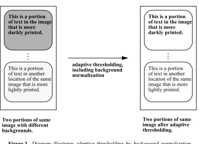
White and Rohrer [White and Rohrer 83] describe an adaptive thresholding algorithm for
separat-ing characters from background. The threshold is continuously changed through the image by
estimating the background level as a two-dimensional running-average of local pixel values taken
for all pixels in the image. (See Figure 3.) Mitchell and Gillies [Mitchell and Gillies 89] describe
a similar thresholding method where background white level normalization is first done by
esti-mating the white level and subtracting this level from the raw image. Then, segmentation of
char-acters is accomplished by applying a range of thresholds and selecting the resulting image with
the least noise content. Noise content is measured as the sum of areas occupied by components
that are smaller and thinner than empirically determined parameters. Looking back at the results
of binarization for different thresholds in Figure 1, it can be seen that the best threshold selection
yields the least visible noise. The main problem with any adaptive binarization technique is the
choice of window size. The chosen window size should be large enough to guarantee that a large
enough number of background pixels are included to obtain a good estimate of average value, but
not so large as to average over nonuniform background intensities. However, often the features in
the image vary in size such that there are problems with fixed window size. To remedy this,
domain dependent information can be used to check that the results of binarization give the
expected features (a large blob of an ON-valued region is not expected in a page of smaller
sym-bols, for instance). If the result is unexpected, then the window size can be modified and
2.2.3: Choosing a Thresholding Method
Whether global or adaptive thresholding methods are used for binarization, one can never expect
perfect results. Depending on the quality of the original, there may be gaps in lines, ragged edges
on region boundaries, and extraneous pixel regions of ON and OFF values. This fact that
process-ing results will not be perfect is generally true with other document processprocess-ing methods, and
indeed image processing in general. The recommended procedure is to process as well as possible
at each step of processing, but to defer decisions that don’t have to be made until later steps to
avoid making irreparable errors. In later steps there is more information as a result of processing
to that point, and this provides greater context and higher level descriptions to aid in making
cor-rect decisions, and ultimately recognition. Deferment, when possible, is a principle appropriate
for all stages of document analysis (except, of course, the last).
This is a portion of text in the image that is more
darkly printed.
This is a portion of text in another location of the same image that is more lightly printed.
This is a portion of text in the image that is more
darkly printed.
This is a portion of text in another location of the same image that is more lightly printed.
. . .
Two portions of same image with different backgrounds.
Two portions of same image after adaptive thresholding.
adaptive thresholding, including background normalization
Figure 3. Diagram illustrates adaptive thresholding by background normalization.
Original image on left has portions of text with different average
back-ground values. The image on the right shows that the backback-grounds have
been eliminated leaving only ON on OFF.
A number of different thresholding methods have been presented in this section. It is the case that
no single method is best for all image types and applications. For simpler problems where the
image characteristics do not vary much within the image or across different images, then the
sim-pler methods will suffice. For more difficult problems of noise or varying image characteristics,
more complex (and time-consuming) methods will usually be required. Commercial products
vary in their thresholding capabilities. Today’s scanners usually perform binarization with respect
to a fixed threshold. More sophisticated document systems provide manual or automatic
h9istogram-based techniques for global thresholding. The most common use of adaptive
thresh-olding is in special purpose systems used by banks to image checks. The best way to choose a
method at this time is first by narrowing the choices by the method descriptions, then just
experi-menting with the different methods and examining their results.
Because there is no “best” thresholding method, there is still room for future research here. One
problem that requires more work is to identify thresholding methods or approaches that best work
on documents with particular characteristics. Many of the methods described above were not
for-mulated in particular for documents, and their performance on them is not well known.
Docu-ments have characteristics, such as very thin lines that will favor one method above another.
Related to this is how best to quantify the results of thresholding. For text, one way is to perform
optical character recognition on the binarized results and measure the recognition rate for
differ-ent thresholds. Another problem that requires further work is that of multi-thresholding.
Some-times documents have not two, but three or more levels of intensities. For instance, many journals
contain highlighting boxes within the text, where the text is against a background of a different
gray level or color. While multi-thresholding capabilities have been claimed for some of the
meth-ods discussed above, not much dedicated work has been focused on this problem.
For other reviews and more complete comparisons of thresholding methods, see [Sahoo 1988,
O’Gorman 1994] on global and multi-thresholding techniques, and [Trier and Taxt 1995] on
adap-tive techniques.
We suggest just manually setting a threshold when the documents are similar and testing is
per-formed beforehand. For automatic, global threshold determination, we have found (in [O’Gorman
1994]) that the moment-preserving method [Tsai 1986] works well on documents. For adaptive
comparison on these adaptive methods. For multi-thresholding, the method [Reddi 1984] is
appropriate if the number of thresholds is known, and the method [O’Gorman 1994] if not.
References
1. D. Mason, I.J. Lauder, D. Rutoritz, G. Spowart, “Measurement of C-bands in human
chromo-somes”, Computers in Biology and Medicine, Vol. 5, 1975, 179-201.
2. J.S. Weszka, A. Rosenfeld, “Histogram modification for threshold selection”, IEEE Trans.
Systems, Man, and Cybernetics, Vol. SMC-9, No. 1, Jan. 1979, p. 38-52.
3. J. Kittler, J. Illingworth, “Minimum error thresholding”, Pattern Recognition, Vol. 19, No. 1,
1986, pp. 41-47.
4. Q-Z. Ye, P-E Danielson, “On minimum error thresholding and its implementations”, Pattern
Recognition Letters, Vol. 7, 1988, pp. 201-206.
5. A.S. Abutaleb, “Automatic thresholding of gray-level pictures using two-dimensional
entropy”, Computer Vision, Graphics, and Image Processing, Vol. 47, 1989, pp. 22-32.
6. N. Otsu, “A threshold selection method from gray-level histograms”, IEEE Trans. Systems,
Man, and Cybernetics, Vol. SMC-9, No. 1, Jan. 1979, pp. 62- 66.
7. S.S. Reddi, S.F. Rudin, H.R. Keshavan, “An optimal multiple threshold scheme for image
seg-mentation”, IEEE Trans. Systems, Man, and Cybernetics, Vol. SMC-14, No. 4, July/Aug,
1984, pp. 661-665.
8. J.N. Kapur, P.K. Sahoo, A.K.C. Wong, “A new method for gray-level picture thresholding
using the entropy of the histogram”, Computer Vision, Graphics, and Image Processing, Vol.
29, 1985, pp. 273-285.
9. W-H. Tsai, “Moment-preserving thresholding: A new approach,” Computer Vision, Grapics,
and Image Processing, Vol. 29, 1985, pp. 377-393.
10. R.G. Casey, K.Y. Wong, “Document analysis systems and techniques”, inImage Analysis Applications, R. Kasturi and M.M. Trivedi (eds), Marcel Dekker, 1990, pp. 1-36.
docu-ment images”, CVGIP: Graphical Models and Image Processing, Vol. 55, No. 3, 1993, pp.
203-217.
12. J.M. White, G.D. Rohrer, “Image thresholding for optical character recognition and other
applications requiring character image extraction”, IBM J. Res. Development, Vol. 27, no. 4,
July 1983, pp. 400- 411.
13. B.T. Mitchell, A.M. Gillies, “A model-based computer vision system for recognizing
hand-written ZIP codes”, Machine Vision and Applications, Vol. 2, 1989, pp. 231-243.
14. P.K. Sahoo, S. Soltani, A.K.C. Wong, Y.C. Chen, “A survey of thresholding techniques”,
Computer Vision, Graphics, and Image Processing, Vol. 41, 1988, pp. 233-260.
15. O.D. Trier and T. Taxt, “Evaluation of binarization methods for document images,” IEEE
Trans. PAMI, Vol. 17, No. 3, Mar. 95, pp. 312-315.
16. L. O’Gorman, “Binarization and multi-thresholding of document images using connectivity”,
2.3: Noise Reduction
Keywords: filtering, noise reduction, salt-and-pepper noise, filling, morphological processing, cellular processing
After binarization, document images are usually filtered to reduce noise. Salt-and-pepper noise
(also called impulse and speckle noise, or just dirt) is a prevalent artifact in poorer quality
docu-ment images (such as poorly thresholded faxes or poorly photocopied pages). This appears as
iso-lated pixels or pixel regions of ON noise in OFF backgrounds or OFF noise (holes) within ON
regions, and as rough edges on characters and graphics components. (See Figure 1.) The process
of reducing this is called “filling”. The most important reason to reduce noise is that extraneous
features will otherwise cause subsequent errors in recognition. Another reason is that noise
reduc-tion reduces the size of the image file, and this in turn reduces the time required for subsequent
processing and storage. The objective in the design of a filter to reduce noise is that it remove as
much of the noise as possible while retaining all of the signal.
2.3.1: Morphological and Cellular Processing
Morphological [Serra 1982, Haralick 1987, Haralick 1992] and cellular processing [Preston 1979]
are two families of processing methods by which noise reduction can be performed. (These
meth-Figure 1. Illustration of letter “e” with salt-and-pepper noise. On the left, the letter is
shown with its ON and OFF pixels as “X”s and blanks, and on the right the
ods are much more general than for just the noise reduction application mentioned here, but we
leave further description of the methods to the references.) The basic morphological or cellular
operations are erosion and dilation. Erosion is the reduction in size of ON-regions. This is most
simply accomplished by peeling off a single-pixel layer from the outer boundary of all ON
regions on each erosion step. Dilation is the opposite process, where single-pixel, ON-valued
lay-ers are added to boundaries to increase their size. These operations are usually combined and
applied iteratively to erode and dilate many layers. One of these combined operations is called
opening, where one or more iterations of erosion are followed by the same number of iterations of
dilation. The result of opening is that boundaries can be smoothed, narrow isthmuses broken, and
small noise regions eliminated. The morphological dual of opening is closing. This combines one
or more iterations of dilation followed by the same number of iterations of erosion. The result of
closing is that boundaries can be smoothed, narrow gaps joined, and small noise holes filled. See
Figure 2 for an illustration of morphological operations.
2.3.2: Text and Graphics Noise Filters
For documents, more specific filters can be designed to take advantage of the known
characteris-tics of the text and graphics components. In particular, we desire to maintain sharpness in these
document components —not to round corners and shorten lengths, as some noise reduction filters
will do. For the simplest case of single-pixel islands, holes, and protrusions, these can be found by
passing a3 x 3sized window over the image that matches these patterns [Shih and Kasturi 1988], then filled. For noise larger than one-pixel, the kFill filter can be used [O'Gorman 1992].
In lieu of including a paper on noise reduction, we describe the kFill noise reduction method in
more detail. Filling operations are performed within akxksized window that is applied in raster-scan order, centered on each image pixel. This window comprises an inside (k-2) x (k-2) region called the core, and the4(k-1)pixels on the window perimeter, called the neighborhood. The fill-ing operation entails settfill-ing all values of the core to ON or OFF dependent upon pixel values in
the neighborhood. The decision on whether or not to fill with ON (OFF) requires that all core
val-ues must be OFF (ON), and depends on three variables, determined from the neighborhood. For a
fill-value equal to ON (OFF), thenvariable is the number of ON- (OFF-) pixels in the neighbor-hood, thecvariable is the number of connected groups of ON-pixels in the neighborhood, and the
X X X X
X X X X
X X X X
X X X X
X
X
X X
X X
X X X X
X X X X
X X X X
X X X X
erosion dilation
opening
X X X
X X X X
X X X
X X X X
X
X
X X X X
X X X X
X X X X
X X X X X X X X
X X X X X X X X X X X X X X X X X X X X X X X X X X X X X X X X X X
X X X
X X X X X X X dilation erosion closing b) c)
Figure 2. Morphological processing. The structuring element in (a) is centered on each
pixel in the image and pixel values are changed as follows. For erosion, an
ON-valued center pixel is turned OFF if the structuring element is over one
or more OFF pixels in the image.For dilation, an OFF-valued center pixel is
turned ON if the structuring element is over one or more ON pixels in the
image. In (b), erosion is followed by dilation; that combination is called
opening. One can see that the isolated pixel and the spur have been removed
in the final result. In (c), dilation is followed by erosion; that combination is
called closing. One can see that the hole is filled, the concavity on the border
is filled, and the isolated pixel is joined into one region in the final result. a)
X X X
X X X
X X X
conditions are met:
The conditions on n and r are set as functions of the window size k such that the text features described above are retained. The stipulation thatc = 1ensures that filling does not change con-nectivity (i.e. does not join two letters together, or separate two parts of the same connected
let-ter). Noise reduction is performed iteratively on the image. Each iteration consists of two
sub-iterations, one performing ON-fills, and the other OFF-fills. When no filling occurs on two
con-secutive sub-iterations, the process stops automatically. An example is shown in Figure 3.
The kFill filter is designed specifically for text images to reduce salt-and-pepper noise while
maintaining readability. It is a conservative filter, erring on the side of maintaining text features
versus reducing noise when those two conflict. To maintain text quality, the filter retains corners
on text of 90oor less, reducing rounding that occurs for other low-pass spatial filters. The filter has akparameter (the kin “kFill”) that enables adjustment for different text sizes and image resolu-tions, thus enabling retention of small features such as periods and the stick ends of characters.
Since this filter is designed for fabricated symbols, text, and graphics, it is not appropriate for
binarized pictures where less regularly shaped regions and dotted shading (halftone) are prevalent.
A drawback of this filter — and of processes that iterate several times over the entire image in
general — is that the processing time is expensive. Whether the expenditure of applying a filter
such as this in the preprocessing step is justified depends on the input image quality and the
toler-ance for errors due to noise in subsequent steps.
Most document processing systems perform rudimentary noise reduction by passing 3x3 filter
masks across the image to locate isolated ON and OFF pixels. For more extensive descriptions of
these techniques in document systems, see [Modayur 1993] for use of morphology in a music
reading system, and [Story 1992] for the use of kFill in an electronic library system.
c = 1
References
1. J. Serra,Image Analysis and Mathematical Morphology, Academic Press, London, 1982.
2. R.M. Haralick, S.R. Sternberg, X. Zhuang, “Image analysis using mathematical morphology”,
IEEE Trans. PAMI, Vol 9, July 1987, pp. 532-550.
3. R. M. Haralick, L. G. Shapiro,Computer and Robot Vision,Addison-Wesley, Reading, Mass., 1992.
Figure 3. Results of kFill filter for salt-and-pepper noise reduction. The original
noisy image is shown at the top left. The top right shows ON pixel removal,
the bottom left shows OFF pixel filling, and the final image is shown in the
4. K. Preston, Jr., M.J.B. Duff, S. Levialdi, P.E. Norgren, J-i. Toriwaki, “Basics of cellular logic
with some applications in medical image processing”, Proc. IEEE, May, 1979, pp. 826-855.
5. C-C. Shih, R. Kasturi, “Generation of a line-description file for graphics recognition”', Proc.
SPIE Conf. on Applications of Artificial Intelligence, 937:568-575, 1988.
6. L. O'Gorman, “Image and document processing techniques for the RightPages Electronic
Library System”', Int. Conf. Pattern Recognition (ICPR), The Netherlands, Sept. 1992, pp.
260-263.
7. B. R. Modayur, V. Ramesh, R. M. Haralick, L. G. Shapiro, “MUSER - A prototype music
score recognition system using mathematical morphology”, Machine Vision and
Applica-tions, Vol. 6, No. 2, 1993, pp.
8. G. Story, L. O'Gorman, D. Fox, L.L. Schaper, H.V. Jagadish, “The RightPages image-based
electronic library for alerting and browsing”, IEEE Computer, Vol. 25, No. 9, Sept., 1992, pp.
2.4: Thinning and Distance Transform
Keywords: thinning, skeletonizing, medial axis transform, distance transform
2.4.1: Thinning
Thinning is an image processing operation in which binary valued image regions are reduced to
lines that approximate the center lines, or skeletons, of the regions. The purpose of thinning is to
reduce the image components to their essential information so that further analysis and
recogni-tion are facilitated. For instance, the same words can be handwritten with different pens giving
different stroke thicknesses, but the literal information of the words is the same. For many
recog-nition and analysis methods where line tracing is done, it is easier and faster to trace along
one-pixel wide lines than along wider ones. Although the thinning operation can be applied to binary
images containing regions of any shape, it is useful primarily for “elongated” shapes versus
con-vex, or “blob-like” shapes. Thinning is commonly used in the preprocessing stage of such
docu-ment analysis applications as diagram understanding and map processing. In Figure 1, some
images are shown whose contents can be analyzed well due to thinning, and their thinning results
are also shown here.
Note should be made that thinning is also referred to as “skeletonizing” and core-line detection in
the literature. We will use the term “thinning” to describe the procedure, and thinned line, or
skel-eton, to describe the results. A related term is the “medial axis”. This is the set of points of a
region in which each point is equidistant to its two closest points on the boundary. The medial axis
is often described as the ideal that thinning approaches. However, since the medial axis is defined
only for continuous space, it can only be approximated by practical thinning techniques that
oper-ate on a sampled image in discrete space.
The thinning requirements are formally stated as follows: 1) connected image regions must thin to
connected line structures, 2) the thinned result should be minimally eight-connected (explained
below), 3) approximate endline locations should be maintained, 4) the thinning results should
approximate the medial lines, and 5) extraneous spurs (short branches) caused by thinning should
be minimized. That the results of thinning must maintain connectivity as specified by requirement
1 is essential. This guarantees an equal number of thinned connected line structures as the number
should always contain the minimal number of pixels that maintain eight-connectedness. (A pixel
is considered eight-connected to another pixel if the second pixel is one of the eight closest
neigh-bors to it.) Requirement 3states that the locations of endlines should be maintained. Since
thin-ning can be achieved by iteratively removing the outer boundary pixels, it is important not to also
Figure 1.Original images on left and thinned image results on right. a) The letter “m”.
b) A line diagram. c) A fingerprint image.
a)
b)
iteratively remove the last pixels of a line. This would shorten the line and not preserve its
loca-tion. Requirement 4 states that the resultant thin lines should best approximate the medial lines of
the original regions. Unfortunately, in digital space, the true medial lines can only be
approxi-mated. For instance, for a 2-pixel wide vertical or horizontal, the true medial line should run at the
half-pixel spacing along the middle of the original. Since it is impossible to represent this in
digi-tal image space, the result will be a single line running at one side of the original. With respect to
requirement 5, it is obvious that noise should be minimized, but it is often difficult to say what is
noise and what isn't. We don't want spurs to result from every small bump on the original region,
but we do want to recognize when a somewhat larger bump is a feature. Though some thinning
algorithms have parameters to remove spurs, we believe that thinning and noise removal should
be performed separately. Since one person’s undesired spur may be another’s desired short line, it
is best to perform thinning first, then, in a separate process, remove any spurs whose length is less
than a specified minimum.
The basic iterative thinning operation is to examine each pixel in an image within the context of
its neighborhood region of at least3 x 3pixels and to “peel” the region boundaries, one pixel layer at a time, until the regions have been reduced to thin lines. (See [Hilditch 1969] for basic 3 x 3
thinning, and [O'Gorman 1990] for generalization of the method tok x ksized masks.) This pro-cess is performed iteratively — on each iteration every image pixel is inspected, and single-pixel
wide boundaries that are not required to maintain connectivity or endlines are erased (set to OFF).
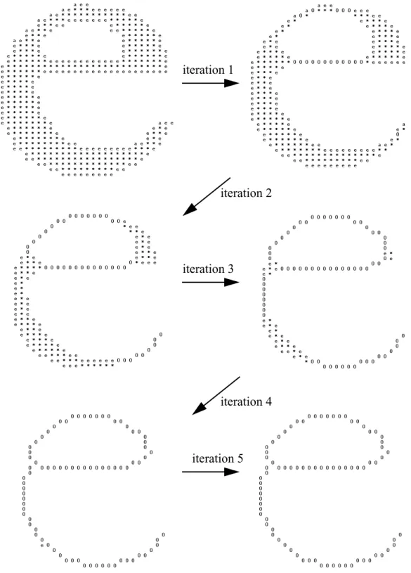
In Figure 2, one can see how, on each iteration, the outside layer of 1-valued regions is peeled off
in this manner, and when no changes are made on an iteration, the image is thinned.
Unwanted in the thinned image are isolated lines and spurs off longer lines that are artifacts due to
the thinning process or noise in the image. Some thinning methods, e.g. [Arcelli and di Baja 85],
require that the binary image is noise filtered before thinning because noise severely degrades the
effectiveness and efficiency of this processing. However noise can never be totally removed, and,
as mentioned, it is often difficult to distinguish noise from the signal in the earlier stages. An
alter-native approach is to thin after rudimentary noise reduction, then perform noise reduction with
higher level information. Segments of image lines between endpoints and junctions are found, and
descriptive parameters (length, type as classified by junctions or endlines at the ends of the
iteration 1
iteration 2
iteration 3
iteration 4
iteration 5
Figure 2. Sequence of five iterations of thinning on letter “e”. On each iteration a
layer of the outer boundaries is peeled off. On iteration 5, the end is
contextual information is then used to remove the line artifacts.
Instead of iterating through the image for a number of times that is proportional to the maximum
line thickness, thinning methods have been developed to yield the result in a fixed number of steps
[Arcelli and di Baja 85, Arcelli and di Baja 89, Sinha 87]. This is computationally advantageous
when the image contains thick objects that would otherwise require many iterations. For these
non-iterative methods, skeletal points are estimated from distance measurements with respect to
opposite boundary points of the regions (see next section on distance transformation). Some of
these methods require joining the line segments after thinning to restore connectivity, and also
require a parameter estimating maximum thickness of the original image lines so that the search
for pairs of opposite boundary points is spatially limited. In general, these non-iterative thinning
methods are less regularly repetitive, not limited to local operations, and less able to be pipelined,
compared to the iterative methods; and these factors makes their implementation in
special-pur-pose hardware less appropriate.
Algorithms have also been developed for extracting thin lines directly from gray-level images of
line drawings by tracking along gray-level ridges, that is without the need for binarization
[Wat-son et al. 84]. These have the advantage of being able to track along ridges whose peak intensities
vary throughout the image, such that binarization by global thresholding would not yield
con-nected lines. However, a problem with tracking lines on gray-scale images is following false
ridges (the gray-scale equivalent of spurs), which results in losing track of the main ridge or
requires computationally expensive backtracking. Binarization and thinning are the methods most
commonly used for document analysis applications because they are well understood and
rela-tively simple to implement.
For recent overview papers on thinning, see [Lam 1992, Lam 1995]. For a reference on thinning
applied specifically to documents, see [Eckhardt 1991].
2.4.2: Distance Transformation
The distance transform is a binary image operation in which each pixel is labeled by the shortest
distance from it to the boundary of the region within which it is contained. One way this can be
used is to determine the shortest path from a given interior point to the boundary. It can also be
This thinned image, complete with distance values, has more information than simply the thinned
image without distance information. It can be used as a concise and descriptive representation of
the original image from which line widths can be obtained or the original image can be
recon-structed. Results of the distance transform are shown in Figure 3.
There are two general approaches to obtaining the distance transformation. One is similar to the
iterative thinning method described above. On each iteration, boundaries are peeled from regions.
But, instead of setting each erased pixel value to OFF, they are set to the distance from the original
boundary. Therefore, on the first iteration (examining 3 x 3 sized masks), erased boundaries are set to zero. On the second iteration, any erased core pixels will have a distance of 1 for vertical or
horizontal distance to a boundary point, or for diagonal distance to a boundary point. On the
third and subsequent iterations, each pixel’s distance value is calculated as the sum of the smallest
distance value of a neighboring pixel plus its distance to that neighbor. When a core can no longer
be thinned, it is labeled with its distance to the closest boundary.
The second approach requires a fixed number of passes through the image. To obtain the integer
approximation of the Euclidean distance, two passes are necessary. The first pass proceeds in
ras-ter order, from the top row to the bottom row, left to right on each row. The distances are
propa-gated in a manner similar to that above, but because the direction of the raster scan is from top left
to bottom right, these first iteration values are only intermediate values— they only contain
dis-tance information from above and to the left. The second pass proceeds in reverse raster order,
from bottom right to top left, where the final distance values are obtained now taking into account
the distance information from below and to the right as well. For further treatments of distance
transformations, see [Borgefors 1984, Borgefors 1986, Arcelli and di Baja1992].
The iterative method is a natural one to use if iterative thinning is desired. As mentioned above,
thinning is only appropriate for elongated regions, and if the distance transform of an image
con-taining thick lines or more convex regions is desired, the fixed-pass method is more appropriate.
The fixed-pass method can also be used as a first step toward thinning. For all of these distance
transformation methods, since distance is stored in the pixel, attention must be paid that the
dis-tance does not exceed the pixel word size, usually a byte. This problem is further exacerbated
since floating point distance is approximated by integer numbers usually by scaling the floating
point number up (e.g. 1.414 would become 14). This word size consideration is usually not a
Figure 3. Distance transform. Top letter “e” shows pixel values equal to distance to
closest border, except for midline pixels (shown in lower picture), which
problem for images of relatively thin, elongated regions, but may be a problem for larger regions.
Thinning is available on virtually all commercial graphics analysis systems. The particular
method varies — there are many, many different thinning methods — but it is usually iterative and
uses 3x3 or 3x4 sized masks. Most systems take advantage of a fast table look-up approach for the
mask operations. These are implemented in software or in hardware for more specialized (faster
and more expensive) machines.
References
1. C.J. Hilditch, “Linear skeletons from square cupboards”, Machine Intelligence 4, 1969, pp.
403-420.
2. L. O'Gorman, “k x k Thinning”, CVGIP, Vol. 51, pp. 195-215, 1990.
3. C. Arcelli, G. Sanniti di Baja, “A width-independent fast thinning algorithm”, IEEE Trans.
Pattern Recognition and Machine Intelligence, Vol. PAMI-7:4, 1985, pp. 463-474.
4. C. Arcelli, G. Sanniti di Baja, “A one-pass two-operation process to detect the skeletal pixels
on the 4-distance transform”, IEEE Trans. Pattern Recognition and Machine Intelligence, Vol.
11:4, 1989, pp. 411-414.
5. R. M. K. Sinha, “A width-independent algorithm for character skeleton estimation”,
Com-puter Vision, Graphics, and Image Processing, Vol. 40, 1987, pp. 388-397.
6. L.T. Watson, K. Arvind, R.W. Ehrich, R.M. Haralick, “Extraction of lines and drawings from
grey tone line drawing images”, Pattern Recognition, 17(5):493-507, 1984.
7. L. Lam, S-W. Lee, C.Y. Suen, “Thinning methodologies — A comprehensive survey”, IEEE
Trans. Pattern Analysis and Machine Intelligence, Vol. 14, No. 9, Sept. 1992, pp. 869-885.
8. L. Lam, C.Y. Suen, “An evaluation of parallel thinning algorithms for character recognition,”
IEEE Trans. Pattern Recognition and Machine Intelligence, Vol. 17, No. 9, Sept. 1995, pp.
914-919.
9. U. Eckhardt, G. Maderlechner, “Thinning for document processing,” Int. Conf. Document
10. G. Borgefors, “Distance transformations in arbitrary dimensions”, Computer Vision,
Graph-ics, and Image Processing, Vol. 27, 1984, pp 321-345.
11. G. Borgefors, “Distance transformations in digital images”, Computer Vision, Graphics, and
Image Processing, Vol. 34, 1986, pp. 344-371.
12. C. Arcelli, G.S. diBaja, “Ridge points in Euclidian distance maps,” Pattern Recognition
2.5: Chain Coding and Vectorization
Keywords: chain code, Freeman chain code, Primitives Chain Code (PCC), line and contour compression, topological feature detection, vectorization
2.5.1: Chain Coding
When objects are described by their skeletons or contours, they can be represented more
effi-ciently than simply by ON and OFF valued pixels in a raster image. One common way to do this
is by chain coding, where the ON pixels are represented as sequences of connected neighbors
along lines and curves. Instead of storing the absolute location of each ON pixel, the direction
from its previously coded neighbor is stored. A neighbor is any of the adjacent pixels in the 3x 3
pixel neighborhood around that center pixel (see Figure 1). There are two advantages of coding by
direction versus absolute coordinate location. One is in storage efficiency. For commonly sized
images larger than 256x256, the coordinates of an ON-valued pixel are usually represented as two
16 bit words; in contrast, for chain coding with eight possible directions from a pixel, each
ON-valued pixel can be stored in a byte, or even packed into three bits. A more important advantage in
this context is that, since the chain coding contains information on connectedness within its code,
this can facilitate further processing such as smoothing of continuous curves, and analysis such as
feature detection of straight lines.
Figure 1. For a 3x 3pixel region with center pixel denoted as X, figure shows codes for
chain directions from center pixel to each of eight neighbors: 0 (east), 1
(north-east), 2 (north), 3 (northwest), etc.
A further explanation is required regarding connectedness between pixels. The definition of
con-nected neighbors that we will use here is called eight-concon-nected. That is, a chain can connect from
one pixel to any of its eight closest neighbors in directions 0 to 7 in Figure 1. Other definitions of
X 0
1 2
3
4