Prediction
Alexander Rakhlin and Karthik Sridharan
DRAFT
I Introduction
7
1 About 8
2 An Appetizer: A Bit of Bit Prediction 12
3 What are the Learning Problems? 18
4 Example: Linear Regression 34
II Theory
43
5 Minimax Formulation of Learning Problems 44
5.1 Minimax Basics . . . 45
5.2 Defining Minimax Values for Learning Problems . . . 48
5.3 No Free Lunch Theorems . . . 55
5.3.1 Statistical Learning and Nonparametric Regression . . . 55
5.3.2 Sequential Prediction with Individual Sequences . . . 56
6 Learnability, Oracle Inequalities, Model Selection, and the Bias-Variance Trade-off 58 6.1 Statistical Learning . . . 58
6.2 Sequential Prediction. . . 64
7.1 Motivation . . . 67
7.1.1 Statistical Learning . . . 67
7.1.2 Sequential Prediction . . . 68
7.2 Defining Stochastic Processes. . . 69
7.3 Application to Learning . . . 73
7.4 Symmetrization . . . 74
7.5 Rademacher Averages . . . 79
7.6 Skolemization . . . 81
7.7 ... Back to Learning . . . 81
8 Example: Learning Thresholds 82 8.1 Statistical Learning . . . 82
8.2 Separable (Realizable) Case . . . 84
8.3 Noise Conditions . . . 85
8.4 Prediction of Individual Sequences . . . 86
8.5 Discussion . . . 89
9 Maximal Inequalities 90 9.1 Finite Class Lemmas . . . 90
10 Example: Linear Classes 94 11 Statistical Learning: Classification 97 11.1 From Finite to Infinite Classes: First Attempt . . . 97
11.2 From Finite to Infinite Classes: Second Attempt . . . 98
11.3 The Growth Function and the VC Dimension. . . 99
12 Statistical Learning: Real-Valued Functions 104 12.1 Covering Numbers . . . 104
12.2 Chaining Technique and the Dudley Entropy Integral. . . 108
12.3 Example: Nondecreasing Functions . . . 110
12.4 Improved Bounds for Classification . . . 112
12.5 Combinatorial Parameters. . . 113
12.6 Contraction . . . 117
12.7 Discussion . . . 118
13 Sequential Prediction: Classification 123
13.1 From Finite to Infinite Classes: First Attempt . . . 124
13.2 From Finite to Infinite Classes: Second Attempt . . . 126
13.3 The Zero Cover and the Littlestone’s Dimension . . . 128
13.4 Removing the Indicator Loss, or Fun Rotations with Trees . . . 132
13.5 The End of the Story . . . 134
14 Sequential Prediction: Real-Valued Functions 136 14.1 Covering Numbers . . . 136
14.2 Chaining with Trees. . . 138
14.3 Combinatorial Parameters. . . 140
14.4 Contraction . . . 145
14.5 Lower Bounds . . . 146
15 Examples: Complexity of Linear and Kernel Classes, Neural Networks 148 15.1 Prediction with Linear Classes . . . 149
15.2 Kernel Methods . . . 149
15.3 Neural Networks . . . 151
15.4 Discussion . . . 153
16 Large Margin Theory for Classification 155 17 Regression with Square Loss: From Regret to Nonparametric Estimation156
III Algorithms
157
18 Algorithms for Sequential Prediction: Finite Classes 158 18.1 The Halving Algorithm . . . 15918.2 The Exponential Weights Algorithm . . . 159
19 Algorithms for Sequential Prediction: Binary Classification with Infinite Classes 164 19.1 Halving Algorithm with Margin . . . 164
19.2 The Perceptron Algorithm . . . 166
20.1 Online Linear Optimization . . . 168
20.2 Gradient Descent . . . 169
20.3 Follow the Regularized Leader and Mirror Descent . . . 170
20.4 From Linear to Convex Functions . . . 173
21 Example: Binary Sequence Prediction and the Mind Reading Machine 174 21.1 Prediction with Expert Advice . . . 175
21.2 Blackwell’s method . . . 175
21.3 Follow the Regularized Leader . . . 178
21.4 Discussion . . . 180
21.5 Can wederivean algorithm for bit prediction? . . . 181
21.6 The Mind Reading Machine . . . 184
22 Algorithmic Framework for Sequential Prediction 186 22.1 Relaxations . . . 188
22.1.1 Follow the Regularized Leader / Dual Averaging . . . 191
22.1.2 Exponential Weights . . . 193
22.2 Supervised Learning . . . 195
23 Algorithms Based on Random Playout, and Follow the Perturbed Leader198 23.1 The Magic of Randomization . . . 198
23.2 Linear Loss . . . 199
23.2.1 Example: Follow the Perturbed Leader on the Simplex . . . 201
23.2.2 Example: Follow the Perturbed Leader on Euclidean Balls . . . 203
23.2.3 Proof of Lemma 23.2 . . . 204
23.3 Supervised Learning . . . 205
24 Algorithms for Fixed Design 206 24.1 ... And the Tree Disappears . . . 206
24.2 Static Experts . . . 208
24.3 Social Learning / Network Prediction . . . 209
24.4 Matrix Completion / Netflix Problem . . . 209
25 Adaptive Algorithms 210 25.1 Adaptive Relaxations . . . 210
IV Extensions
213
26 The Minimax Theorem 214
26.1 When the Minimax Theorem Does Not Hold . . . 215
26.2 The Minimax Theorem and Regret Minimization . . . 216
26.3 Proof of a Minimax Theorem Using Exponential Weights . . . 218
26.4 More Examples . . . 220
26.5 Sufficient Conditions for Weak Compactness. . . 221
27 Two Proofs of Blackwell’s Approachability Theorem 224 27.1 Blackwell’s vector-valued generalization and the original proof . . . . 225
27.2 A non-constructive proof . . . 228
27.3 Discussion . . . 230
27.4 Algorithm Based on Relaxations: Potential-Based Approachability . . 230
28 From Sequential to Statistical Learning: Relationship Between Values and Online-to-Batch 231 28.1 Relating the Values . . . 231
28.2 Online to Batch Conversion . . . 233
29 Sequential Prediction: Better Bounds for Predictable Sequences 235 29.1 Full Information Methods . . . 237
29.2 Learning The Predictable Processes . . . 240
29.3 Follow the Perturbed Leader Method . . . 242
29.4 A General Framework of Stochastic, Smoothed, and Constrained Ad-versaries . . . 242
30 Sequential Prediction: Competing With Strategies 243 30.1 Bounding the Value with History Trees . . . 244
30.2 Static Experts . . . 248
30.3 Covering Numbers and Combinatorial Parameters . . . 249
30.4 Monotonic Experts . . . 250
30.5 Compression and Sufficient Statistics . . . 253
1
About
This course will focus on theoretical aspects ofStatistical LearningandSequential Prediction. Until recently, these two subjects have been treated separately within the learning community. The course will follow a unified approach to analyzing learning in both scenarios. To make this happen, we shall bring together ideas from probability and statistics, game theory, algorithms, and optimization. It is this blend of ideas that makes the subject interesting for us, and we hope to convey the excitement. We shall try to make the course as self-contained as possible, and pointers to additional readings will be provided whenever necessary. Our target audience is graduate students with a solid background in probability and linear algebra.
“Learning” can be very loosely defined as the “ability to improve performance after observing data”. Over the past two decades, there has been an explosion of both applied and theoretical work on machine learning. Applications of learning methods are ubiquitous: they include systems for face detection and face recogni-tion, prediction of stock markets and weather patterns, speech recognirecogni-tion, learn-ing user’s search preferences, placement of relevant ads, and much more. The success of these applications has been paralleled by a well-developed theory. We shall call this latter branch of machine learning – “learning theory”.
Why should one care about machine learning? Many tasks that we would like computers to perform cannot be hard-coded. The programs have to adapt. The goal then is to encode, for a particular application, as much of the domain-specific knowledge as needed, and leaveenough flexibilityfor the system to improve upon observing data.
knowledge from the expert. The goal of learning theory then is to develop gen-eral guidelines and algorithms, and prove guarantees about learning performance under various natural assumptions.
A number of interesting learning models have been studied in the literature, and a glance at the proceedings of a learning conference can easily overwhelm a newcomer. Hence, we start this course by describing a few learning problems. We feel that the differences and similarities between various learning scenarios become more apparent once viewed as minimax problems. The minimax frame-work also makes it clear where the “prior knowledge” of the practitioner should be encoded. We will emphasize the minimax approach throughout the course.
What separates Learning from Statistics? Both look at data and have similar goals. Indeed, nowadays it is difficult to draw a line. Let us briefly sketch a few his-torical differences. According to [55], in the 1960’s it became apparent that clas-sical statistical methods are poorly suited for certain prediction tasks, especially those characterized by high dimensionality. Parametric statistics, as developed by Fisher, worked well if the statistician couldmodel the underlying process generat-ing the data. However, for many interesting problems (e.g. face detection, char-acter recognition) the associated high-dimensional modeling problem was found to be intractable computationally, and the analysis given by classical statistics – inadequate. In order to avoid making assumptions on the data-generating mech-anism, a newdistribution-freeapproach was suggested. The goal within the ma-chine learning community has therefore shifted from beingmodel-centricto be-ingalgorithm-centric. An interested reader is referred to the (somewhat extreme) point of view of Breiman [13] for more discussion on the two cultures, but let us say that in the past 10 years both communities benefited from sharing of ideas. In the next lecture, we shall make the distinctions concrete by formulating the goals of nonparametric estimation and statistical learning as minimax problems. Fur-ther in the course, we will show that these goals are not as different as it might first appear.
Support Vector Machines and AdaBoost) are often considered to be state-of-the art methods for prediction problems. These methods adhere to the philosophy that, for instance, for classification problems one should not model the distributions but rather model the decision boundary. Arguably, this accounts for success of many learning methods, with the downside that interpretability of the results is often more difficult. The term “learning” itself is a legacy of the field’s strong con-nection to computer-driven problems, and points to the fact that the goal is not necessarily that of “estimating the true parameter”, but rather that of improving performance with more data.
In the past decade, research in learning theory has been shifting to sequen-tial problems, with a focus on relaxing any distributional assumptions on the ob-served sequences. A rigorous analysis of sequential problems is a large part of this course. Interestingly, most research on sequential prediction (or,online learning) has been algorithmic: given a problem, one would present a method and prove a guarantee for its performance. In this course, we present a thorough study of inherent complexities of sequential prediction. The goal is to develop it in com-plete parallel with the classical results of Statistical Learning Theory. As an added (and unexpected!) bonus, the online learning problem will give us an algorithmic toolkit for attacking problems in Statistical Learning.
We start the course by presenting a fun bit prediction problem. We then pro-ceed to list in a rather informal way a few different learning settings, some of which are not “learning” per se, but quite closely related. We will not cover all these in the course, but it is good to see the breadth of problems anyway. In the follow-ing lecture, we will go through some of these problems once again and will look at them through the lens of minimax. As we go through the various settings, we will point out three key aspects:(a) how data are generated; (b) how the performance is measured; and (c) where we place prior knowledge.
Before proceeding, let us mention that we will often make over-simplified state-ments for the sake of clarity and conciseness. In particular, our definitions of re-search areas (such as Statistical Learning) are bound to be more narrow than they are. Finally, these lecture notes reflect a personal outlook and may have only a thin intersection with the reality.1
1For a memorable collection of juicy quotes, one is advised to take a course with J. Michael
the set of all distributions on some setAby∆(A).
Deviating from the standard convention, we sometimes denote random vari-ables by lower-case letters, but we do so only if no confusion can arise. This is done for the purposes of making long equations appear more tidy.
Expectation with respect to a random variableZwith distributionpis denoted by EZ orEZ∼p. We caution that in the literatureEZ is sometimes used to denote a conditional expectation; our notation is more convenient for the problems we have in mind.
The inner product between two vectors is written variably asa·b, or〈a,b〉, or asaT
b. The set of all functions fromXtoYis denoted byYX. The unitLp ball in
Rd will be denoted byBd
2
An Appetizer: A Bit of Bit Prediction
We start our journey by describing the simplest possible scenario – that of “learn-ing” with binary-valued data. We put “learn“learn-ing” in quotes simply because various research communities use this term for different objectives. We will now describe several such objectives with the aim of drawing parallels between them later in the course. Granted, the first three questions we ask are trivial, but the last one is not – so read to the end!
What can be simpler than the Bernoulli distribution? Suppose we observe a sample y1, . . . ,yndrawn i.i.d. from such a distribution with an unknown bias p∈ (0, 1). The goal ofestimationis to provide a guess of the population parameterp
based on these data. Any kindergartner (raised in a Frequentist family) will happily tell us that a reasonable estimate ofpis the empirical proportion of ones
¯
yn, 1
n
n
X
t=1
yi,
while a child from a Bayesian upbringing will likely integrate over a prior and add a couple of extra 0’s and 1’s to regularize the solution for smalln. What can we say about the quality of ¯ynas an estimate ofp? From the Central Limit Theorem (CLT), we know that1|p−y¯n| =OP
¡ n−1/2¢
, and in particular
E|p−y¯n| =O(n−1/2) .
For thepredictionscenario, suppose again that we are giveny1, . . . ,yn drawn independently from the Bernoulli distribution with an unknown bias p, yet the
1For a sequence of random variablesy
1, . . . ,yn, . . . and positive numbersa1, . . . ,an, . . ., the
nota-tionyn=OP(an) means that for anyδ>0, there exists anR>0 such thatP
¡
|yn| >Ran
¢
same distribution as measured by the indicator of a mistakeI©yb6=y ª
. Sincey is a random variable itself, the decisionybincurs the expected cost ofEI
© b y6=yª
. We may compare this cost to the cost of the best decision
EI© b y6=yª
− min y0∈{0,1}EI
© y06=yª
and observe that the minimum is attained aty∗=I©
p≥1/2ª
and equal to
min y0∈{0,1}EI
© y06=yª
=min{p, 1−p}.
Also note that the minimum can only be calculated with the knowledge ofp. How-ever, since ¯yn is a good estimate ofp, we can approximate the minimizer quite well. It is rather clear that we should predict with the majority voteyb=I
©
¯
yn≥1/2
ª
. Why?
Our third problem is that ofsequential prediction with i.i.d. data. Suppose we observe the i.i.d. Bernoulli drawsy1, . . . ,yn, . . . in a stream. At each time instant
t, having observed y1, . . . ,yt−1, we are tasked with making thet-th prediction. It
shouldn’t come as a surprise that by going with the majority vote
b yt =I©
¯
yt−1≥1/2
ª
once again, the average prediction cost
1
n
n
X
t=1
EI© b yt6=yt
ª
−min{p, 1−p}
can be shown to beO(n−1/2) once again. Another powerful statement can be de-duced from the strong Law of Large Numbers (LLN):
lim sup n→∞
µ
1
n
n
X
t=1
I©ybt6=yt ª
−min{ ¯yn, 1−y¯n}
≤0 almost surely . (2.1)
That is to say, for almost all sequences (under the probabilistic model), the average number of mistakes is (asymptotically) no more than the smallest between the proportion of zeros and proportion of ones in the sequence.
without any assumptions on the way the sequence is generated.
Ponder for a minute on the meaning of this statement. It says that whenever the proportion of 1’s (or 0’s) in the sequence is, say, 70%, we should be able to correctly predict at least roughly 70% of the bits. It is not obvious that such a strategy even exists without any assumptions on the generative process of the data!
It should be observed that the method of predictingI©y¯t−1≥1/2
ª
at steptno longer works. In particular, it fails on the alternating sequence 0, 1, 0, 1, . . . since
I©
¯
yt−1≥1/2
ª
=1−yt. Such an unfortunate sequence can be found for any deter-ministic algorithm: simply let yt be the opposite of what the algorithm outputs given y1, . . . ,yt−1. The only remaining possibility is to search for a randomized
al-gorithm. The “almost sure” part of (2.1) will thus be with respect to algorithm’s randomization, while the sequences are now deterministic. The roles have magi-cally switched!
Letqt ∈[0, 1] denote the bias of the distribution from which we draw the ran-domized prediction ybt. Let us present two methods that achieve the goal (2.1).
First method is defined with respect to a horizonn, which is subsequently doubled upon reaching (the details will be provided later), and the distribution is defined as
qt=
exp©−n−1/2Pt−1
s=1(1−ys)
ª
exp©
−n−1/2Pt−1
s=1ys
ª
+exp©
−n−1/2Pt−1
s=1(1−ys)
ª
We do not expect that this randomized strategy means anything to the reader at this point. And if it does – the next one should not. Here is a method due to D. Blackwell. LetLt−1be the point in [0, 1]2with coordinates ( ¯yt−1, ¯ct−1) where ¯ct−1=
1−t−11Pt−1
s=1I
© b ys6=ys
ª
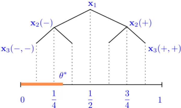
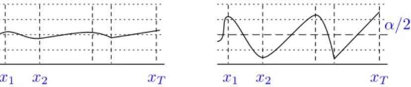
is the proportion of correct predictions of the algorithm thus far. IfLt−1is in the left or the right of the four triangles composing [0, 1]2(see figure
below), chooseqt to be 0 or 1; otherwise draw a line from the center throughLt−1
and letqt be the value when this line intersects thex-axis. Why does this method work? Does it come from some principled way of solving such problems? We defer the explanation of the method to Chapter21, but, meanwhile, we hope that these brief algorithmic sketches piqued readers’ interest.
Lt 1
(0,0) q
t
can one hope to find a prediction method that achieves
∀y1, . . . ,yn, E
·
1
n
n
X
t=1
I© b yt 6=yt
ª ¸
≤φn(y1, . . . ,yn) (2.2)
In other words, what types of functions of the sequence upper bound the aver-age number of mistakes an algorithm makes on that sequence? Of course, the smaller we can make this function, the better. But clearly φn ≡0 is an impossi-bly difficult task (forcing us to make zero mistakes on any sequence) andφn≡1 is a trivial requirement achieved by any method. Hence,φnshould be somewhere in-between. If we guess the bit by flipping a coin, the expected number of mis-takes is 1/2, and thusφn≡1/2 is feasible too. What about the more interesting (non-constant) functions?
Let’s only focus only on those functions which are “stable” with respect to a coordinate flip:
|φn(a)−φn(a0)| ≤1/n for all a,a0∈{0, 1}n with ka−a0k1=1 (2.3)
For such functions, the answer (due to T. Cover) might come as a surprise:
Proposition 2.1. For a stable (in the sense of (2.3)) functionφn, there exists an al-gorithm achieving(2.2)for all sequencesif and only if
Eφn(y1, . . . ,yn)≥1/2 (2.4)
where the expectation is under theuniformdistribution on{0, 1}n.
Let us show the easy direction. Fix an algorithm that enjoys (2.2). Suppose now that y1, . . . ,yn are taken to be unbiased coin flips. Since the decision ybt is
made before yt is revealed, the expected loss is clearly EI
© b yt 6=yt
ª
other direction is rather unexpected: for anyφnwith the aforementioned property, there exists an algorithm that enjoys (2.2). We will show this in Section25.2.
The above characterization is quite remarkable, as we only need to lower bound the expected value under the uniform distribution to ensure existenceof an al-gorithm. Roughly speaking, the characterization says that a function φn can be smaller than 1/2 for some sequences, but it then must be compensated by allow-ing for more errors on other sequences. This opens up the possibility of targetallow-ing those sequences we expect to observe in the particular application. If we can en-gineer a functionφnthat is small on those instances, the prediction algorithm will do well in practice. Of course, if we do have the knowledge that the sequence is i.i.d., we may simply choose min{ ¯yn, 1−y¯n} as the benchmark. The ability to get good performance for non-i.i.d. sequences appears to be a powerful statement, and it foreshadows the development in these notes. We refer the reader to the exercises below to gain more intuition about the possible choices ofφn.
So far, we have considered prediction of binary sequences in a “vacuum”: the problem has little to do with any phenomenon that we might want to study in the real world. While it served as a playground for the introduction of several con-cepts, such a prediction problem is not completely satisfying. One typically has someside informationandprior knowledgeabout the situation, and these consid-erations will indeed give rise to the complexity and applicability of the methods discussed in the course.
At this point, we hope that the reader has more questions than answers. Where do these prediction algorithms come from? How does one develop them in a more complicated situation? Why doesn’t the simple algorithm from the i.i.d. world work? Is there a real difference in terms of learning rates between the individual sequence prediction and prediction with i.i.d. data? How far can the individual sequence setting be pushed in terms of applicability? These and many more ques-tions will be addressed in the course.
We strongly encourage you to attempt these problems. If you solved all three, you are in a good shape for the course!
E 1 n
X
t=1
I©ybt6=yt ª
≤min{ ¯yn, 1−y¯n}+C n−1/2
for any sequence. Can we take any C >0? Find a good (or nearly best) con-stantC. (Hint: consult known bounds on lengths of random walks). Observe that
Emin{ ¯yn, 1−y¯n} by itself is less than 1/2 and thus the necessary additional term is a compensation for “fluctuations”.
P Exercise (??): Suppose that for eachi=1, . . . ,k,φin: {0, 1}n→Rsatisfies (2.4) as well as the stability condition (2.3). What penalty should we add to
min i∈{1,...,k}φ
i n
to make sure the new “best ofk” complexity satisfies (2.4)? Verify (2.3) for the new function and conclude that there must exist an algorithm that behaves not much worse than the given k prediction algorithms. (Hint: Use the stability property (2.3) together with McDiarmid inequality (see Appendix, LemmaA.1) to conclude subgaussian tails for|Eφin−φin|. Use union bound and integrate the tails to arrive at the answer.)
3
What are the Learning Problems?
Statistical Learning
Let us start with the so-calledsupervised learning. Within this setting, data are represented by pairs of input and output (also called predictor and response) vari-ables, belonging to some sets XandY, respectively. Atraining set, or abatch of data, will be denoted by
{(Xt,Yt)}nt=1=(Xn,Yn)∈Xn×Yn.
It is after observing this set that we hope to learn something about the relationship between elements ofXandY.
For instance,Xt can be a high-dimensional vector of gene expression for thet -th patient andYtcan stand for the presence or absence of diabetes. Such classifica-tionproblems focus on binary “labels”Y={0, 1}.Regression, on the other hand, fo-cuses on real-valued outputs, whilestructured predictionis concerned with more complex spaces of outcomes. The main (though not exclusive) goal of Statistical Learning is inprediction; that is, “learning” is equated with the ability to better predict they-variable from thex-variable after observing the training data.
So, how is our learning performance evaluated? Suppose, after observing the data, we can summarize the “learned” relationship betweenXandYvia a hypoth-esis yb:X→Y. We may think of ybas a “decision” from the setDof all functions mapping inputs to outputs. We then consider the average error in predicting Y
fromXbased on this decision:
E£
`(yb, (X,Y)) ¯ ¯Xn,Yn
¤
(3.1)
where the expectation is over the random draw of (X,Y) according to PX×Y and independently of (Xn,Yn), and`:D×(X×Y)→Ris someloss functionwhich mea-sures the gravity of the mistake. As an example, if we are learning to classify spam emails, the measure of performance is how well we predict the spam label of an email drawn at random from the population of all emails.
IfY={0, 1}, we typically consider theindicator loss
`(yb, (X,Y))=I ©
b
y(X)6=Yª
or its surrogates (defined in later lectures), and for regression problems it is com-mon to study thesquare loss
`(yb, (X,Y))=(yb(X)−Y)
2
and theabsolute loss
`(yb, (X,Y))= |yb(X)−Y|.
Since the training data {(Xt,Yt)}nt=1 are assumed to be a random draw, these examples might be misleading by chance. In this case, we should not penalize the learner. Indeed, a more reasonable goal is to ask that the average
E`(yb, (X,Y))=E ©
E©
`(yb, (X,Y)) ¯ ¯Xn,Yn
ªª
(3.2)
of (3.1) under the draw of training data be small. Alternatively, the goal might be to show that (3.1) is small with high probability. It is important to keep in mind thatyb
is random, as it depends on the data. We will not write this dependence explicitly, but the hat should remind us of the fact.
IfPX×Y were known, finding ybthat minimizesE`(yb, (X,Y)) would be a matter
not available to us and the only information we receive about it is through the training sample. What do we do then? Well, as stated, the task of producingybwith
a small error (3.2) is unsurmountable in general. Indeed, we mentioned that there is no universal learning method, and we just asked for exactly that! Assumptions or prior knowledge are needed.
Where do we encode this prior knowledge about the task? This is where Sta-tistical Learning (historically) splits from classical Statistics. The latter would typ-ically posit a particular form of the distributionPX×Y, called a statistical model. The goal is then to estimate the parameters of the model. Of course, one can make predictions based on these estimates, and we discuss this (plug-in) approach later. However, it is not necessary to perform the estimation step if the end-goal is pre-diction. Indeed, it can be shown quite easily (see [21]) that the goal of estimation is at least as hard as the goal of prediction for the problem of classification. For regression, the relationship between estimation and prediction with squared loss amounts to the study of well-specified and misspecified models and will be dis-cussed in the course.
In contrast to the modeling approach, the classical work of Vapnik and Chervo-nenkis is of adistribution-freenature. That is, the prior knowledge does not enter in the form of an assumption onPX×Y, and our learning method should be “suc-cessful” for all distributions. Instead, practitioner’s “inductive bias” is realized by selecting a classFof hypothesesX→Ythat is believed to explain well the relation-ship between the variables. There is not much room to circumvent the problem of no universal learning algorithm! Requiring the method to be successful for all distributions means that the very notion of “successful” has to include the prior knowledgeF. A natural requirement is to minimize the lossrelativetoF:
E`(yb, (X,Y))−inf f∈F
E`(f, (X,Y)) (3.3)
Such a performance metric is calledregret, and the loss function downshifted by the best in classFis calledexcess loss. Hence, “learning” is defined as the ability to provide a summary yb:X→Yof the relationship between X andY such that
the expected loss is competitive with the loss of the best “explanation” within the classF. Generally, we do not requireybitself to lie inF, yet the learning algorithm
that producesybwill certainly depend on the benchmark set. We shall sometimes
It can be argued that the distribution-free formulation in (3.3) should be used with a “growing” setF, and idea formalized by Structural Risk Minimization and the method of sieves. A related idea is to estimate from data the parameters ofF itself. Such methods will be discussed in the lecture onmodel selectiontowards the end of the course. In the next lecture, we will discuss at length the merits and drawbacks of the distribution-free formulation. For further reading on Statistical Learning Theory, we refer the reader to [12,3,38].
Let us also mention that independently of the developments by Vapnik and Chervonenkis, a learning framework was introduced in 1984 by Valiant within the computer science community. Importantly, the emphasis was made on polynomi-ally computable learning methods, in the spirit of Theoretical Computer Science. This field ofComputational Learning Theorystarted as a distribution-dependent
(that is, non-distribution-free) study of classification. Fix a collectionFof map-pingsX→{0, 1}. Suppose we can make a very strong prior knowledge assumption that one of the functions inFin fact exactly realizes the dependence between X
and the labelY. Since (X,Y) is a draw fromPX×Y, the assumption of
Y=f(X) for some f ∈F (3.4) translates into the assumption that the conditional distributionPY|X=a=δf(a). It
is then possible to characterize classesFfor which the probability of error
P(yb(X)6=f(X))=E|yb(X)−f(X)| (3.5)
can be made small for some learning mechanism yb. This setting is termed real-izable and forms the core of the original PAC (Probably Approximately Correct) framework of Valiant [53]. Of course, this is not a distribution-free setting. It was the papers of Haussler [25] and then Kearns et al [32] that extended the PAC frame-work to be distribution-free (termedagnostic).
In an intermediate setting between realizable and agnostic, one assumeslabel noise; that is, givenX, the binary labelYis “often” equal to f(X), except for some cross-over probability:
∃f ∈F such that for anyx∈X, PY|X(Y6=f(a)|X=a)<η<1/2 (3.6)
Let us briefly mention a more general framework. Let us remove the assumption that data are of the formX×Yand instead write it as some abstract setZ. This setting includes the so-calledunsupervised learning tasks such as clustering and density estimation. Given the data {Zt}nt=1, the learning method is asked to sum-marize what it had learned by some elementyb∈D, yet we do not requireDto be
a class of functionsX→Y, and instead treat it as an abstract set. The quality of the prediction is assessed through a loss function`:D×Z→R, and we assume a fixed unknown distributionPZonZ. As before, the data are assumed to be an i.i.d. sample fromPZ, and the performance measure
E`(yb,Z)
is evaluated under the random drawZ∼PZ.
The setting we described is almost too general. Indeed, the problem of finding
b
ysuch thatE`(yb,Z) is small is considered in such areas as Statistical Decision
The-ory, Game TheThe-ory, and Stochastic Optimization. One can phrase many different frameworks under any one of these umbrellas, and our aim is simply to make the connections clear.
Nonparametric Regression
Nonparametric regression withfixed design assumes that the data {(Xt,Yt)}nt=1∈ (X×Y)nconsist of predictor-response pairs, whereXt’s are fixed a priori (e.g. evenly spaced on the interval) and Yt = f(Xt)+²t, for independent zero-mean noise²t and some function f :X→ Y. For random design, we assume (as in Statistical Learning Theory) thatXt’s are random and i.i.d. from some marginal distribution
PX, either known or unknown to us. Then, givenXt, we assumeYt =f(Xt)+²t, and this defines a joint distributionPXf×Y =PX×PYf|X parametrized byf.
Given the data, letybsummarize what has been learned. In statistical language,
we construct an estimateybof the unknownf parametrizing the distributionP
f X×Y. The typical performance measure is the lossE(yb(X)−f(X))
2or some otherp-norm.
Instead of integrating with respect to the marginal PX, the fixed-design setting only measures (yb(X)−f(X))
2on the design points.
More generally, the notion of loss can be defined through the function`:D×
E`(yb,f)=E E `(yb,f)¯X ,Y (3.7)
is small.
Clearly, the study of (3.7) needs to depend on properties ofF, which embodies the prior assumptions about the problem. This prior knowledge is encoded as a distributional assumption onPXf×Y in a similar way to the “label noise setting” of PAC learning discussed above. In the next lecture, we will make the distinction between this setting and Statistical Learning even more precise.
Of course, this simple sketch cannot capture the rich and interesting field of nonparametric statistics. We refer to [52] and [57] for thorough and clear exposi-tions. These books also study density estimation, which we briefly discuss next.
Density Estimation
Suppose that we observe i.i.d. data {Zt}nt=1∈Znfrom a distributionPZf with a den-sity f. The goal is to construct an estimateyb:Z→Rof this unknown density. The error of the estimate is measured by, for instance, the integrated mean squared error (under the Lebesgue measure)
E ½Z
(yb(z)−f(z))2d z ¾
or via the Kullback-Leibler divergence
E`(yb,f)= Z
f(z) log f(z)
b
y(z)d z=E
½
logf(Z)
b y(Z)
¾
=E©(−logyb(Z))−(−logf(Z)) ª
.
The KL divergence as a measure of quality of the estimator corresponds to a (nega-tive) log loss`(f,z)= −logf(z) which is central to problems in information theory. Once again, construction of optimal estimators depends on the particular char-acteristics that are assumed aboutf, and these are often embodied via the distribution-dependent assumption f ∈F. The characteristics that lead to interesting state-ments are often related to the smoothness of densities inF.
to be available all at once as a batch, and the “performance” is assessed throughyb
with respect to the unknown distribution.
We now move beyond these “static” scenarios. In sequential problems we typi-cally “learn” continuously as we observe more and more data, and there is a greater array of problems to consider. One important issue to look out for is whether the performance is measured throughout the sequence or only at the end. Problems also differ according to the impact the learner has through his actions. Yet another aspect is the amount of information or feedback the learner receives. Indeed, se-quential problems offers quite a number of new challenges and potential research directions.
Universal Data Compression and Conditional
Probabil-ity Assignment
In this scenario, suppose that a stream ofz1,z2, . . . is observed. For simplicity,
sup-pose that allzt take on values in a discrete setZ. There are two questions we can ask: (1) how can we sequentially predict eachzthaving observed the prefix {zs}ts=−11? and (2) how can we compress this sequence? It turns out that these two questions are very closely related.
As in the setting of density estimation, suppose that the sequence is gener-ated according to some distribution f on finite (or infinite) sequences in Zn (or
Z∞), with f in some given set of distributionsF.1 Once again,F embodies our
assumption about the data-generating process, and the problem presented here is distribution-dependent. Later, we will introduce the analogue of universal pre-diction forindividual sequences, where the prior knowledgeFwill be moved to the “comparator” in a way similar to distribution-free Statistical Learning.
So, how should we measure the quality of the “learner” in this sequential prob-lem? SinceZt’s are themselves random draws, we might observe unusual sequences, and should not be penalized for not being able to predict them. Hence, the mea-sure of performance should be an expectation over the possible sequences. On
1Note the slight abuse of the notation: previously, we have usedPf do denote the distribution
assignment”. A natural measure of error at timetis then the expected log-ratio
E ½
logf(Z|Z t−1)
b yt(Z)
¯ ¯ ¯ ¯
Zt−1
¾
or some other notion of distance between the actual and the predicted distribu-tion. When the mistakes are averaged over a finite-horizon timen, the measure of performance becomes
1
n
n
X
t=1
E ½
logf(Z|Z t−1)
b yt(Z)
¯ ¯ ¯ ¯
Zt−1
¾ = 1
nE ½
logf(Z n)
b y(Zn)
¾
, (3.8)
where ybcan be thought of either as a joint distribution over sequences, or as a collection ofnconditional distributions for all possible prefixes. If data are i.i.d., the measure of performance becomes an averaged version of the one introduced for density estimation with KL divergence.
There are two main approaches to ensuring that the expected loss in (3.8) is small: (1) the plug-in approach involves estimating at each step the unknown dis-tribution f ∈Fand using it to predict the next element of the sequence; (2) the mixture approach involves a Bayesian-type averaging of all distributions inF. It turns out that the second approach is superior, a fact that is known in statistics as suboptimality of selectors, or suboptimality of plug-in rules. We refer the inter-ested reader to the wonderful survey of Merhav and Feder [40]. In fact, the reader will find that many of the questions asked in that paper are echoed (and some-times answered) throughout the present manuscript.
Prediction of Individual Sequences
Let us discuss a general setting of sequential prediction, and then particularize it to an array of problems considered within the fields of Statistics, Game Theory, Information Theory, and Computer Science.
At an abstract level, suppose we observe a sequencez1,z2, . . .∈Zof data and
need to make decisions yb1,yb2, . . .∈Don the fly. Suppose we would like to lift the
tion. In fact, let us assume thatthere is no distribution governing the evolution of z1,z2, . . .. The sequence is then calledindividual2. This surprising twist of events
might be difficult for statisticians to digest, and we refer to the papers of Phil Dawid on prequential statistics for more motivation. The (weak) prequential principle states that “any criterion for assessing the agreement between Forecaster and Na-ture should depend only on the actual observed sequences and not further on the strategies which might have produced these” [20].
If there is only one sequence, then how do we evaluate learner’s performance? A sensible way is to score learner’s instantaneous loss on round t by `(ybt,zt),
where the decision ybt must be chosen on the basis ofz
t−1, but notz
t. Averaging overn, the overall measure of performance on the given sequence is
1
n
n
X
t=1
`(ybt,zt). (3.9)
Just as in our earlier exposition on statistical learning, it is easy to show that mak-ing the above expression small is an impossible goal even in simple situations. Some prior knowledge is necessary, and two approaches can be taken to make the problem reasonable. As we describe them below, notice that they echo the as-sumptions of “correctness of the model” and the alternative competitive analysis of statistical learning.
Assumption of Realizability Let us consider the supervised setting: Z=X×Y. We make an assumption that the sequence z1, . . . ,zn is only “in part” individual. That is, the sequence x1, . . . ,xn is indeed arbitrary, yet yt is given by yt = f(xt) for some f ∈F. Additional “label noise” assumption has also been considered in the literature. Under the “realizability” assumption, the goal of minimizing (3.9) is feasible, as will be discussed later in the course. However, a much richer setting is the following.
Competitive Analysis This is the most studied setting, and the philosophy is in a sense similar to that of going from distribution-dependent to distribution-free
2Strictly speaking, the termindividual sequence, coming from information theory, refers to
off ):
Regret= 1 n
n
X
t=1
`(ybt,zt)−inf
f∈F 1
n
n
X
t=1
`(f,zt) (3.10)
That is, the average loss of the learner is judged by the yardstick, which is the best fixed decision from the setFthat we could have “played” for then rounds. The reader probably noticed that we started to use a game-theoretic lingo. Indeed, the scenario has a very close relation to game theory.
More generally, we can define regret with respect to a setΠof strategies, where each strategyπ∈Πis a sequence of mappingsπt from the past to the set of deci-sionsF:
Regret= 1 n
n
X
t=1
`(ybt,zt)−inf π∈Π
1
n
n
X
t=1
`(πt(zt−1),zt) (3.11)
From this point of view, (3.10) is regret with respect to a set of constant strategies. The reader should take a minute to ponder upon the meaning of regret. If we care about our average loss (3.9) being small and we are able to show that regret as defined in (3.11) is small, we would be happy if we knew that the comparator loss is in fact small. But when is it small? When the sequences are well predicted by some strategy from the setΠ. Crucially, we arenotassuming that the data are generated according to a process related in any way toΠ! All we are saying is that,
if we can guarantee smallness of regret for all sequences andif the comparator term captures the nature of sequences we observe, our average loss is small. Nev-ertheless, it is important that the bound on regret that is proved for all individual sequences will hold... well... for all sequences. Just the interpretation might be unsatisfactory.
the prior knowledge into the comparator term. The upper bounds one gets can be more conservative in general. How much more conservative will be a subject of interest in this course. Furthermore, the duality between assuming a form of a data-generating process versus competing with the related class of predictors is very intriguing and has not been studied much. We will phrase this duality pre-cisely and show a number of positive results.
Summarizing, it should now be clear what the advantages and disadvantages of the regret formulation are: we have a setup of sequential decision-making with basically no assumptions that would invalidate our result, yet smallness of regret is “useful” whenever the comparator term is small. On the downside, protection against all models leads to more conservative results than one would obtain mak-ing a distributional assumption.
For a large part of the course we will study the regret notion (3.10) defined with respect to a single fixed decision. Hence, the upper bounds we prove for regret will hold for all sequences, but will be more useful for those sequences on which a single decision is good on all the rounds. What are such sequences? There is def-initely a flavor of stationarity in this assumption, and surely the answer depends on the particular form of the loss`. We will also consider regret of the form
Regret= 1 n
n
X
t=1
`(ybt,zt)− inf
(g1,...,gn)
1
n
n
X
t=1
`(gt,zt) (3.12)
where the infimum is taken over “slowly-changing” sequences. This can be used to model an assumption of a non-stationary but slowly changing environment, without ever assuming that sequences come from some distribution. It should be noted that it is impossible in general to have an average loss comparable to that of the best unrestricted sequence (g1, . . . ,gn) of optimal decisions that changes on every round.3
The comprehensive book of Cesa-Bianchi and Lugosi [16] brings together many of the settings of prediction of individual sequences, and should be consulted as a supplementary reading. It is, in fact, after picking up this book in 2007 that our own interests in the field sparked. The following question was especially bother-some: why do upper bounds on regret defined in (3.10) look similar to those for 3Some algorithms studied in computer science do enjoycompetitive-ratiotype bounds that
this question. We will show the connections between the two scenarios, as well as the important differences.
Let us mention that we will study an even more difficult situation than de-scribed so far: the sequence will be allowed to be picked not before the learning process, butduring the process. In other words, the sequence will be allowed to change depending on the intermediate “moves” (or decisions) of the learner. This is a good model for learning in the environment on which learner’s actions have an effect. We need to carefully define the rules for this, as to circumvent the so-called Cover’s impossibility result. Since the sequence will be allowed to evolve in the worst-case manner, we will model the process as a game against anadaptive adversary. A good way to summarize the interaction between the learner and the adversary (environment, Nature) is by specifying the protocol:
Sequential prediction with adaptive environment
At each time stept=1 ton,
• Learner choosesybt∈Dand Nature simultaneously chooseszt ∈Z
• Player suffers loss`(ybt,zt) and both players observe (ybt,zt)
In the case of a non-adaptive adversary, the sequence (z1, . . . ,zn) is fixed before the game and is revealed one-by-one to the player.
We remark that the nameindividual sequencetypically refers to non-adaptive adversaries, yet we will use the name for the both adaptive and non-adaptive sce-narios. There is yet another word we will abuse throughout the course: “predic-tion”. Typically, prediction refers to the supervised setting when we are trying to predict some target responseY. We will use prediction in a rather loose sense, and synonymously with “decision making”: abstractly, we “predict” or “play” or “make decision” or “forecast”ybton roundteven if the decision spaceDhas nothing to do
with the outcome spaceZ. Finally, we remark that “online learning” is yet another name often used for sequential decision-making with the notion of regret.
Online Convex Optimization
as well slightly abuse the notation and equivalently rewrite`(yb,z) as`z(yb) or even
z(yb), wherez:D→Ris a convex function andD=Fis a convex set. The latter
no-tation makes it a bit more apparent that we are stepping into the world of convex optimization.
Regret can now be written as
Regret= 1 n
n
X
t=1
zt(ybt)−inf
f∈F 1
n
n
X
t=1
zt(f) (3.13)
where the sequencez1, . . . ,znis individual (also calledworst-case), and eachzt(f) is a convex function.
At the first sight, the setting seems restricted, yet it turns out that the majority of known regret-minimization scenarios can be phrased this way. We briefly men-tion that methods from the theory of optimizamen-tion, such as gradient descent and mirror descent, can be employed to achieve small regret, and these methods are often very computationally efficient. These algorithms are becoming the meth-ods of choice for large scale problems, and are used by companies such as Google. When data are abundant, it is beneficial to process them in a stream rather than as a batch, which means we are in the land of sequential prediction. Being able to relax distributional assumptions is also of great importance for present-day learn-ing problems. It is not surprislearn-ing that online convex optimization has been a “hot” topic over the past 10 years.
The second part of this course will focus on methods for studying regret in con-vex and non-concon-vex situations. Some of our proofs will be algorithmic in nature, some – nonconstructive. The latter approach is particularly interesting because the majority of the results in the literature so far have been of the first type.
Multiarmed Bandits and Partial Information Games
Theexploration-exploitation dilemmais a phenomenon usually associated with situation where an action that brings the most “information” does not necessar-ily yield the best performance. This dilemma does not arise when the aim is re-gret minimization and the outcomezt is observed after predictingybt. Matters
choice of armi at time stept results in a random rewardrt drawn independently from the distributionpi with support on [0, 1] and meanµi. The goal is to mini-mize regret of not knowing the best arm in advance: maxi∈{1...k}µin−Pnt=1rt. An
optimal algorithm for this problem has been exhibited by Lai and Robbins [34]. Switching to losses instead of rewards, the goal can be equivalently written as min-imization of expected regret
E ½
1
n
n
X
t=1
`(ybt,zt)
¾ −inf
f∈F
E ½
1
n
n
X
t=1
`(f,zt)
¾
where `(yb,z)=yb,z ®
, D=F={e1, . . . ,ek} the set of standard basis vectors, and expectation is over i.i.d. draws of zt ∈[0, 1]k according to the product of one-dimensional reward distributionsp1×. . .×pk. Crucially, the decision-maker only observes the loss`(yb,z) (that is, one coordinate ofz) upon choosing an arm. The setting is the most basic regret-minimization scenario for i.i.d. data where the exploration-exploitation dilemma arises. The dilemma would not be present had we defined the goal as that of providing the best hypothesis at the end, or had we observed the full reward vectorzt at each step.
Interestingly, one can consider the individual sequence version of the multi-armed bandit problem. It is not difficult to formulate the analogous goal: mini-mize regret
E (
1
n
n
X
t=1
`(ybt,zt)−inf
f∈F 1
n
n
X
t=1
`(f,zt)
)
where`(yb,z)=
b y,z®
, the learner only observes the value of the loss, and the se-quence z1, . . . ,zn is arbitrary. Surprisingly, it is possible to develop a strategy for minimizing this regret. Generalizations of this scenario have been studied re-cently, and we may formulate the following protocol:
Bandit online linear optimization
At each time stept=1 ton,
• Learner choosesybt∈Dand Nature simultaneously chooseszt ∈Z
• Player suffers loss`(ybt,zt)=
b yt,zt
®
generality, yet the question of optimal rates here is still open. In the stochastic setting with a fixed i.i.d. distribution for rewards, however, we may formulate the problem as minimizing regret
E (
1
n
n
X
t=1
z(ybt)−inf
f∈F
z(f)
)
(3.14)
wherez is an unknown convex function and the learner receives a random draw from a fixed distribution with meanz(ybt) upon playingybt. An optimal (in terms of the dependence onn) algorithm for this problem has been recently developed. Note that (3.14) basically averages the values of the unknown convex function
z at the trajectoryyb1, . . . ,ybn and compares it to the minimum value of the func-tion over the setF. The reader will recognize this as a problem of optimization, but with the twist of measuring average error instead of the final error. This twist leads to the exploration-exploitation tradeoff which is absent if we can spendn it-erations gathering information about the unknown function and then output the final answer based on all the information.
Convex Optimization with Stochastic and
Determinis-tic Oracles
Convex optimization is concerned with finding the minimum of an unknown con-vex functionz(yb) over a setF, which we assume to be a convex set. The optimiza-tion process consists of repeatedly queryingyb1, . . . ,ybn∈D=Fand receiving some information (from the Oracle) about the function at each query point. For deter-ministic optimization, this information is noiseless, while for stochastic optimiza-tion it is noisy. For the zero-th order optimizaoptimiza-tion, the noiseless feedback to the learner (optimizer) consists of the valuez(ybt), while for stochastic optimization
the feedback is typically a random draw from a distribution with meanz(ybt).
Sim-ilarly, first order noiseless information consists of a (sub)gradient ofzatybt, while
the stochastic feedback provides this value only on average. The deterministic op-timization goal is to minimizez(ybn)−inff∈Fz(f). In the stochastic case the goal
is, for instance, in expectation:
E (
z(ybn)−inf f∈F
z(f)
)
A particularly interesting stochastic optimization problem is to minimize the convex function
˜
z(yb)=E`(yb,Z) (3.15)
Even if distribution is known, the integration becomes computationally difficult wheneverZ⊂Rd with even modest-size d [41]. The idea then is to generate an i.i.d. sequence Z1, . . . ,Zn and use it in place of the difficult-to-compute integral. Since given the random draws we still need to perform optimization, we suppose there is an oracle that returns random (sub)gradientsG(yb,Z) given the query (yb,Z)
such that
EG(yb,Z)∈∂z˜(yb)=E∂yb`(yb,Z).
Given access to such information about the function, two approaches can be con-sidered: stochastic approximation (SA) and sample average approximation (SAA). The SAA approach involves directly minimizing
1
n
n
X
t=1
`(yb,Zt)
as a surrogate for the original problem in (3.15). The SA approach consists of tak-ing gradient descent steps of the type ybt+1=ybt−ηG(ybt,Zt) with averaging of the
final trajectory. We refer to [41] for more details.
Note that we have come a full circle! Indeed, (3.15) is the problem of Statis-tical Learning that we started with, except we did not assume convexity of `or
4
Example: Linear Regression
Linear regression is, arguably, the most basic problem that can be considered within the scope of statistical learning, classical regression, and sequential prediction. Yet, even in this setting, obtaining sharp results without stringent assumptions proves to be a challenge. Below, we will sketch similar guarantees for methods in these three different scenarios, and then make some unexpected connections. Us-ing the terminology introduced earlier, we consider thesupervisedsetting, that is
Z=X×Y, whereY=R. LetF=Bd2 be the unit`2ball inRd. Each f ∈Rd can be
thought of as a vector, or as a function f(x)=f ·x, and we will move between the two representations without warning. Consider the square loss
`(f, (x,y))=(f(x)−y)2=(f ·x−y)2
as a measure of prediction quality. In order to show how various settings differ in their treatment of linear regression, we will make many simplifying assumptions along the way in order to present an uncluttered view. In particular, we assume thatnis larger thand.
Classical Regression Analysis
We start with the so-calledfixed designsetting, wherex1, . . . ,xnare assumed to be fixed and onlyYt’s are randomly distributed. Assume alinear model: there exists a
g∗∈Rd such that
Y =Xg∗+²
whereX∈Rn×d the matrix with rowsxt, Y and²the vectors with coordinatesYt and²t, respectively. Let
ˆ
Σ, 1
n
n
X
t=1
xtxtT
be the covariance matrix of the design. Denoting by Dthe set of all functions
X→Y, the goal is to come up with an estimateyb∈Dsuch that
E ½ 1 n n X
t=1
(yb(xt)−g∗(xt))2
¾
(4.2)
is small. With a slight abuse of notation, whenever yb∈R
d, we will write the above
measure as
Ekyb−g
∗k2 ˆ
Σ.
In particular, let
b
y=argmin g∈Rd
1
n
n
X
t=1
(Yt−g·xt)2=argmin g∈Rd
1
n ° °Y −Xg
° °
2
(4.3)
be theordinary least squares estimator, or theempirical risk minimizer, overRd. Then
b y=Σˆ−1
µ
1
n
n
X
t=1
Ytxt
¶ = 1
nΣˆ
−1XT Y
assuming the inverse exists (and use pseudo-inverse otherwise). Multiplying (4.1) on both sides byxt and averaging overt, we find that
g∗=Σˆ−1 µ
1
n
n
X
t=1
(Yt−²t)xt
¶ , and hence E° ° b y−g∗°
°
2 ˆ
Σ=E ° ° ° °
ˆ
Σ−1
µ
1
n
n
X
t=1
²txt
¶° ° ° ° 2 ˆ Σ = 1 nE · ² µ 1
nXΣˆ
−1
XT 
²
whereU has orthonormal columns (orthonormal basis of the column space ofX). Then the measure of performance (4.2) for ordinary least squares is
1
nE ° °UT²
° °
2
≤σ
2d
n
The random design analysis is similar, and theO(d/n) rate can be obtained under additional assumptions on the distribution ofX (see [28]).
CONCLUSION: In the setting of linear regression, we assume a linear relation-ship between predictor and response variables, and obtain anO(d/n) rate for both fixed and random design.
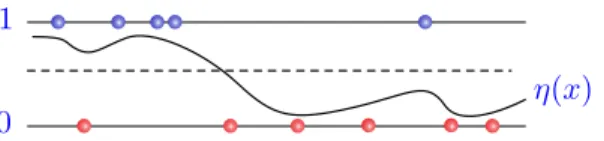
Statistical Learning
In this setting we assume that {(Xt,Yt)}nt=1are i.i.d. from some unknown distribu-tionPX×Y. We placeno prior assumptionon the relationship betweenXandY. In particular,η(a),E[Y|X=a] is not necessarily a linear function inRd. Recall that the goal is to come up withybsuch that
E¡ b
y·X−Y¢2−inf f∈F
E(f ·X−Y)2 (4.4)
is small.
Before addressing this problem, we would like to motivate the goal of compar-ing prediction performance to that inF. Why not simply consider unconstrained minimization as in the previous section? Let
g∗=argmin g∈Rd
E(g·X−Y)2 (4.5)
be the minimizer of the expected error over all ofRd, andybbe the ordinary least
squares, as in (4.3). For anyg,g0∈Rd, using the fact thatη(X)=E[Y|X],
E(g·X−Y)2−E(g0·X−Y)2=E(g·X−η(X))2−E(g0·X−η(X))2. (4.6)
Further,
E(g·X−Y)2−E(g∗·X−Y)2=E(g·X−g∗·X+g∗·X−Y)2−E(g∗·X−Y)2
tions (4.6) and (4.7) give, for anyg ∈Rd, the Pythagoras relationship
kg−ηk2X− kg∗−ηk2X= kg−g∗k2X .
Attempting to control excess loss over all ofRdis equivalent to finding an estimator
b
y that ensures convergence of kyb−g
∗k2
X (which is simply kyb−g
∗k2
Σ) to zero, a
task that seems very similar to the one in the previous section. However, the key difference is that y is no longer a random variable necessarily centered atg∗·X. This makes the goal of estimating g∗ difficult, and is only possible under some conditions. Hence, we would not be able to get a distribution-free result. Let us sketch the argument in [28]: we may write
Σ1/2(
b
y−g∗)=Σ1/2Σˆ−1Σ1/2Eˆ£Σ−1/2X(η(X)−g∗·X)¤+Σ1/2Σˆ−1/2Eˆ£Σˆ−1/2X(Y−η(X))¤
A few observations can be made. First, by optimality ofg∗,E(X(η(X)−g∗·X))=0. Of course, we also haveE(Y−η(X))=0. Further,Σ1/2Σˆ−1Σ1/2can be shown to be tightly concentrated around identity. We refer the reader to [28] for a set of conditions under which the above decomposition gives rise toO(d/n) rates.
Instead of making additional distributional assumptions to make the unre-stricted minimization problem feasible, we can instead turn to the goal of proving upper bounds on (4.4). Interestingly, this objective requires somewhat different techniques. Let us denote by ˆf the empirical minimizer constrained to lie within the set Fand f∗ be the minimizer of the expected loss withinF. As depicted in Figure ??, we may view ˆf and f∗ as projections (although with respect to differ-ent norms) of the unconstrained optimaybandg
∗, respectively, ontoF. The
pro-jections may be closer than the unconstrained minimizers, although by itself this argument is not enough since the inequalities are in the opposite direction:
kf −f∗k2X≤ kf −ηk2X− kf∗−ηkX2 =E¡f ·X−Y¢2−E(f∗·X−Y)2
for any f ∈F(Exercise). With tools developed towards the end of the course, we will be able to show that excess loss (4.4) in the distribution-free setting of Statisti-cal Learning is indeed upper bounded byO(d/n).
We conclude this section by observing that the problem (4.4) falls under the purview of Stochastic Optimization. By writing
E(g·X−Y)2=gTΣ