DISCUSSION PAPER SERIES
Forschungsinstitut zur Zukunft der Arbeit Institute for the Study
Retaining through Training: Even for Older Workers
IZA DP No. 5591March 2011 Matteo Picchio Jan C. van Ours
Retaining through Training:
Even for Older Workers
Matteo Picchio
Tilburg University, CentER, ReflecTand IZA
Jan C. van Ours
Tilburg University, CentER, ReflecT, University of Melbourne, CESifo, CEPR and IZADiscussion Paper No. 5591
March 2011
IZA P.O. Box 7240 53072 Bonn Germany Phone: +49-228-3894-0 Fax: +49-228-3894-180 E-mail: [email protected]Any opinions expressed here are those of the author(s) and not those of IZA. Research published in this series may include views on policy, but the institute itself takes no institutional policy positions. The Institute for the Study of Labor (IZA) in Bonn is a local and virtual international research center and a place of communication between science, politics and business. IZA is an independent nonprofit organization supported by Deutsche Post Foundation. The center is associated with the University of Bonn and offers a stimulating research environment through its international network, workshops and conferences, data service, project support, research visits and doctoral program. IZA engages in (i) original and internationally competitive research in all fields of labor economics, (ii) development of policy concepts, and (iii) dissemination of research results and concepts to the interested public. IZA Discussion Papers often represent preliminary work and are circulated to encourage discussion.
IZA Discussion Paper No. 5591 March 2011
ABSTRACT
Retaining through Training: Even for Older Workers
* This paper investigates whether on-the-job training has an effect on the employability of workers. Using data from the Netherlands we disentangle the true effect of training incidence from the spurious one determined by unobserved individual heterogeneity. We also take into account that there might be feedback from shocks in the employment status to future propensity of receiving firm-provided training. We find that firm-provided training significantly increases future employment prospects. This finding is robust to a number of robustness checks. It also holds for older workers, suggesting that firm-provided training may be an important instrument to retain older workers at work.JEL Classification: C33, C35, J21, J24, M53
Keywords: training, employment, human capital, older workers
Corresponding author: Matteo Picchio Department of Economics Tilburg University PO BOX 90153 5000 LE Tilburg The Netherlands E-mail: [email protected] *
1
Introduction
Active Labour Market Policies (ALMP) aim to increase employment rates by stimulating job finding rates and reducing job separation rates. In recessions ALMP are used to dampen the effects of the downturn in employment. In the recent crisis temporary shorter working hours arrangements, often in combination with increased training of workers, were used as instruments. Indeed several countries reported measures to provide training to existing workers at risk of job loss (OECD,2010).
On-the-job training is an investment by individuals and firms which is aimed at up-grading individuals’ human capital and which might pay back in terms of better labour market performances and higher productivity in the future. Training helps individuals to meet the needs of a changing economic and technological environment, enlarge the spec-trum of competences, increase productivity, send good signals to employers, and thereby avoid unemployment events and return faster at work in case of job loss.
The question whether adult training affects labour market performances and produc-tivity of individuals has been the core of substantial debates and research investigations. A strand of the literature analyses whether training programmes are tools to integrate the unemployed into the work force. Training programmes are found to have a modest or no effect on unemployment exit rates (Gerfin and Lechner,2002;Andrén and Andrén,2006; Crépon et al.,2007;Lechner et al.,2008;Lalive et al.,2008;Sianesi,2008) and on wages (Heckman et al., 1999). Positive effects are instead found on the future employment sta-bility (Crépon et al.,2007;Lechner et al.,2008) andJones et al.(2009) show that training is significantly and positively associated with job satisfaction.
A similar branch of this literature has tried to understand how on-the-job training af-fects wages and other performance measures. Gritz(1993) concludes that participation in training improves the employment prospects, especially for women, the youth, and minorities. Bonnal et al. (1997) report that, in the private sector, on-the-job training in-creases the employment rates, especially for young workers. Bartel(1995) shows that, at firm level, wages and productivity are positively affected by on-the-job training. Finally, several other studies find that on-the-job training has a significantly positive impact on productivity (see, among others,Bartel,1994;Barrett and O’Connell,2001;Conti,2005; Dearden et al.,2006).
In the Netherlands, previous evaluation studies have tried to infer the impact of dif-ferent kind of training programmes on future employment prospects. Ridder(1986) dis-tinguishes between training, recruitment, and employment programmes. He finds that es-pecially women and ethnic minorities benefit from training programmes.Sanders and de Grip(2004) investigate whether training participation might affect low-skilled workers’
firm-internal and firm-external mobility. They find that training increases firm-internal mobility, but it does not affect firm-external employability. Lastly, Pavlopoulos et al. (2009) analyse the effect of training on low pay mobility. They find that training increases the chances for upward wage mobility and therefore improves earnings prospects.
All in all, the effect of training on employment prospects is often found to be some-what disappointing. Either training does not increase job finding rates significantly or even modest negative effects are found (see also Kluve (2010) for a recent overview study). Whereas the effect of training on job finding rates has been studied quite fre-quently, the effect on job separation rates is rarely investigated.1
Using data on the Netherlands from the European Community Household Panel (EC-HP), we investigate whether firm-provided training enhances the probability of retaining workers into the workforce in the Netherlands. From the econometric viewpoint, it is challenging to disentangle the pure effect of training from the spurious one determined by individual unobserved heterogeneity. Unobserved heterogeneity might indeed jointly determine the likelihood of training participation and the labour market performances: motivation, labour market attachment, innate ability. Using semiparametric techniques to control for the endogeneity of training participations, we explicitly model the inter-related dynamics leading to training and determining the future employment prospects. We also take into account that there might be feedback from current employment shocks to individuals’ future probability of receiving firm-provided training. As a result, we are able to estimate policy-relevant effects of on-the-job training participation on employment prospects later in life.
We find that in the Netherlands firm-provided training significantly improves future employability, i.e training leads to retaining.2 We also focus on the effect for older work-ers. As in many other European countries, the labour market position of older workers is cause for concern in the Netherlands, given that the demographic trends are causing an ageing of the workforce and that older workers’ job separations are often a one-way street out of the labour force and into long-term unemployment. We find that older workers who receive training are more likely to remain employed. We suggest that additional on-the-job training of workers, especially older workers, can be influenced by government 1Using cross-country time series data on unemployment rates Boone and van Ours (2009) find that training has a significant negative effect on unemployment. They do not attribute this to the positive effect of training on the job finding rate but to the negative effect on the job separation rate. Training increases the human capital of participants and therefore the quality of their post-unemployment job increases, leading to lower job separation rates.
2In a companion paper,Picchio and van Ours(2011), we show that in the Netherlands firm-sponsored training is affected by labour market imperfections but not by product market competition. If labour mo-bility goes up employers are less willing to invest in training. If product market competition increases employer sponsored training is unaffected.
policy, for example by providing the employers with age-specific subsidies to stimulate firm-provided training. Furthermore, an age-specific firing tax may persuade employers to train older workers, increasing thereby older workers’ employability.
This paper is set up as follows. The data are described in Section 2. Section 3 formal-izes the econometric model and clarifies the identification strategy. The estimation results are presented and discussed in Section 4. Section 5 concludes.
2
Data Description
The data used in this paper are from the 1994–2001 waves of the longitudinal dimension of the ECHP, a rotating panel survey based on harmonized methodology and definitions across several European countries. The ECHP contains nationally representative samples of households and covers a large set of of topics such as work, income, financial situation, housing, family, health, training and education, and social relations. We select data for the Netherlands, where the survey was annually conducted by Statistics Netherlands, under the coordination of Eurostat. The longitudinal ECHP data for the Netherlands comprise a number of individual records that range from 12,000 to 13,000 per year over the time window 1994–2001, for a total of 100,716 records.
From the original Dutch ECHP panel data, we lose the 1994 wave as information on training was not collected in 1994 in the Netherlands. We focus on prime age and older workers, i.e. workers who are older than 26 and younger than 64 years of age and who are either employee or not employed. Self-employed workers are deemed to be structurally different from employees and therefore are excluded from the sample. We drop observations with missing values in the variables used in the econometric analysis and we drop individuals that are not in the sample for at least three consecutive time periods between 1994 and 2001. The latter restriction is due to the fact that we estimate a dynamic model of order one with unobserved effects. Hence, one time period is lost because of the model dynamics. A further period is lost as we will use initial values to correct for initial conditions induced by the presence of unobserved effects.
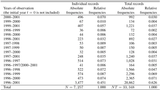
After the application of these sample selection criteria, we have an unbalanced panel of 7,257 individuals, for a total of 33,348 individual-year observations, from 1996 until 2001.3 Table 1 clarifies the structure of our data.
3Whe have an unbalanced panel due to attrition, missing information, and sample renewal for issues of representativeness over time. We assume that attrition and missing information are random. It would have been interesting to use more recent data. Unfortunately, it is not possible to use data the EU database on Statistics on Income and Living Conditions (SILC) as this database does not contain information about training.
Table 1: The Structure of the Unbalanced Panel
Individual records Total records Years of observation Absolute Relative Absolute Relative (the initial yeart= 0is not included) frequencies frequencies frequencies frequencies
2000–2001 496 0.070 992 0.030 1999–2000 67 0.010 134 0.004 1999–2001 407 0.057 1,221 0.037 1998–1999 36 0.006 72 0.002 1998–2000 44 0.006 132 0.004 1998–2001 223 0.032 892 0.027 1997-1998 53 0.009 106 0.003 1997-1999 50 0.007 150 0.005 1997–2000 32 0.005 128 0.004 1997–2001 248 0.035 1,240 0.037 1996–1997 514 0.073 1,028 0.031 1996–1997/2000–2001 41 0.006 164 0.005 1996–1998 522 0.072 1,566 0.047 1996–1999 574 0.087 2,296 0.069 1996–2000 473 0.074 2,365 0.071 1996–2001 3,477 0.451 20,862 0.626 Total N= 7,257 1.000 N T= 33,348 1.000
We are interested in whether and to what extent the employability of a worker – the probability of remaining employed – is affected by firm-provided training. The non-employment indicator is constructed on the basis of the ILO definition of non-employment status. It is denoted by yit and it is equal to 1 if individuali is not in the workforce at
timet and 0 otherwise. The firm-provided training indicator wit is instead equal to 1 if
employeeiattended vocational education courses paid or organized by the firm since the beginning of the previous year and 0 otherwise.4
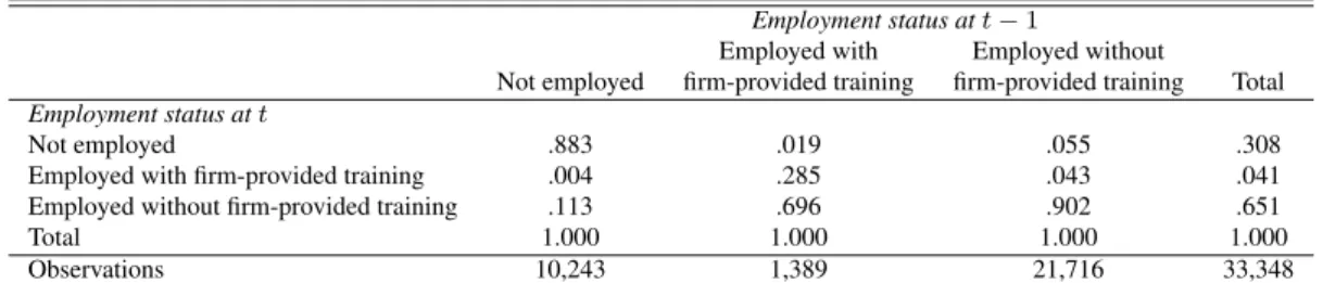
Table 2 reports the probabilities of being out of the workforce conditional and uncon-ditional of previous employment situation. The unconuncon-ditional non-employment probabil-ity is 30.8% and it shows a strong persistence, possibly due to individual observed and unobserved heterogeneity: someone not employed at t−1is almost 20 times as likely not to be employed attas someone employed att−1. The non-employment probability is lower for those who attended some firm-provided training in the past than those who did not: 1.9% against 5.5%. Note that the probability of attending firm-provided training courses seems to be strongly affected by the past employment condition. This might be due to individual observed and unobserved heterogeneity but it might also reflect feed-back effects going from current shocks in the employment status to future probability of attending firm-provided training.
Table 3 displays the observed transitions between employment positions and, as ex-4We build the non-employment indicator on the basis of variables PE003 and PE004 of the ECHP survey. The firm-provided training indicator is built on the basis of variables PT001 and PT017.
Table 2: Raw Conditional and Unconditional Nonemployment Probabilities Employment status att−1
Employed with Employed without
Not employed firm-provided training firm-provided training Total
Employment status att
Not employed .883 .019 .055 .308
Employed with firm-provided training .004 .285 .043 .041 Employed without firm-provided training .113 .696 .902 .651
Total 1.000 1.000 1.000 1.000
Observations 10,243 1,389 21,716 33,348
pected, most of the individuals show a strong persistence in employment. The identifica-tion of the effect of training on employees’ employability comes from observaidentifica-tions out of the diagonal of this transition matrix.
Table 3: Absolute (Relative) Frequencies of Transitions between Labour Market Positions Employment status att−1
Employed with Employed without
Not employed firm-provided training firm-provided training Total
Employment status att
Not employed 9,048 (.271) 26 (.001) 1,194 (.036) 10,268 (.308) Employed with firm-provided training 36 (.001) 396 (.014) 931 (.028) 1,363 (.041) Employed without firm-provided training 1,159 (.035) 967 (.029) 19,591 (.588) 21,717 (.651) Total 10,243 (.307) 1,389 (.042) 21,716 (.651) 33,348 (1.000)
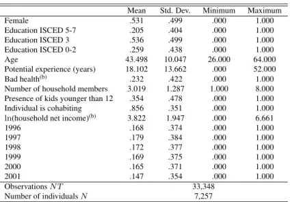
Table 4 presents summary statistics of the outcome variables and of the variables used in the specification of the employment equation. We control for gender, education, age, years of potential work experience, health status, number of household components, pres-ence of children in the household (younger than 12 years old), position in the family, and time indicators.5 The average age is about 43 years with 18 years of potential working
ex-perience. More than 53% of the people in the sample are women, 54% have a secondary degree, and more than 23% do not have a good health situation. On average each house-hold has 3 members, while 35% of the sample has a child younger than 12 years of age in the household. Almost 86% of the people are living in a couple (married or unmarried).
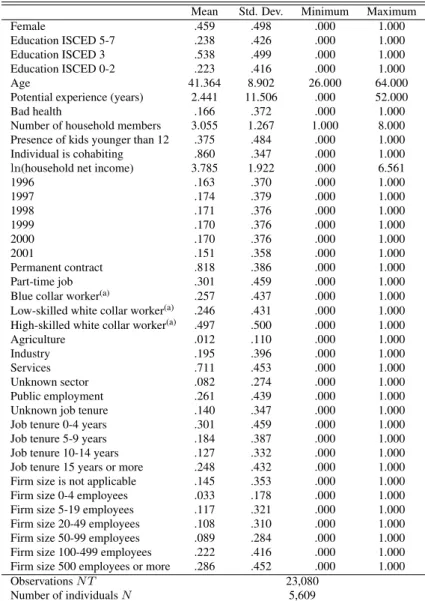
Table 5 shows summary statistics of the covariates entering the training equation for employees. In this case further variables capturing job and employment characteristics are used to explain employees’ probability of receiving firm-provided training: contract arrangement, part-time indicator, occupational dummies, job tenure, and sector and firm 5In the model specification we also included the interactions between gender and presence of children.
Table 4: Summary Statistics of the Pooled Sample
Mean Std. Dev. Minimum Maximum
Female .531 .499 .000 1.000
Education ISCED 5-7 .205 .404 .000 1.000 Education ISCED 3 .536 .499 .000 1.000 Education ISCED 0-2 .259 .438 .000 1.000
Age 43.498 10.047 26.000 64.000
Potential experience (years) 18.102 13.662 .000 52.000
Bad health(b) .232 .422 .000 1.000
Number of household members 3.019 1.287 1.000 8.000 Presence of kids younger than 12 .354 .478 .000 1.000 Individual is cohabiting .856 .351 .000 1.000
ln(household net income)(b) 3.822 1.947 .000 6.661
1996 .168 .374 .000 1.000 1997 .179 .384 .000 1.000 1998 .172 .377 .000 1.000 1999 .169 .375 .000 1.000 2000 .165 .371 .000 1.000 2001 .147 .354 .000 1.000 ObservationsN T 33,348 Number of individualsN 7,257
(a)We build the health indicator on the basis of variable PH001, which reports
self-perceived health. It is equal to one in case of fair, rather bad, or bad health conditions. It is equal to zero in case of either good or very good health conditions.
(b)The household net income is computed from the variables HI100 and PI100. It does
not include the income of the corresponding individual and it is in constant prices (2000 prices). It is deflated by using the Consumer Price Index (CPI), gathered by Statistics Netherlands.
size indicators. About 82% of the employees have a permanent job and more than 30% work on a part-time basis. Almost half of the employees are high-skilled white collar workers, more than 71% work in the service sector, and more than 50% work in firms with more than 100 employees. More than 26% of the workers have a job in the public sector.
3
Econometric Modelling
In this Section we describe a multivariate discrete response model for panel data to inves-tigate whether the employment probability is affected by participation in firm-provided training courses. There are reasons to suspect that the training indicator is a potentially endogenous human capital variable. First, there might be self-selection issues related to unobserved heterogeneity: time-invariant individual characteristics, unobservable by the econometrician, that jointly determine the probability of being at work and participating in training. Innate ability, intelligence, motivations, and labour market attachments are examples of such endowments that, if ignored, may lead to biased parameter estimates (Heckman, 1981;Hyslop, 1999). Second, there might be feedback effects from
employ-Table 5: Summary Statistics of Employees
Mean Std. Dev. Minimum Maximum
Female .459 .498 .000 1.000
Education ISCED 5-7 .238 .426 .000 1.000 Education ISCED 3 .538 .499 .000 1.000 Education ISCED 0-2 .223 .416 .000 1.000
Age 41.364 8.902 26.000 64.000
Potential experience (years) 2.441 11.506 .000 52.000
Bad health .166 .372 .000 1.000
Number of household members 3.055 1.267 1.000 8.000 Presence of kids younger than 12 .375 .484 .000 1.000 Individual is cohabiting .860 .347 .000 1.000
ln(household net income) 3.785 1.922 .000 6.561
1996 .163 .370 .000 1.000 1997 .174 .379 .000 1.000 1998 .171 .376 .000 1.000 1999 .170 .376 .000 1.000 2000 .170 .376 .000 1.000 2001 .151 .358 .000 1.000 Permanent contract .818 .386 .000 1.000 Part-time job .301 .459 .000 1.000
Blue collar worker(a) .257 .437 .000 1.000
Low-skilled white collar worker(a) .246 .431 .000 1.000
High-skilled white collar worker(a) .497 .500 .000 1.000
Agriculture .012 .110 .000 1.000
Industry .195 .396 .000 1.000
Services .711 .453 .000 1.000
Unknown sector .082 .274 .000 1.000
Public employment .261 .439 .000 1.000 Unknown job tenure .140 .347 .000 1.000 Job tenure 0-4 years .301 .459 .000 1.000 Job tenure 5-9 years .184 .387 .000 1.000 Job tenure 10-14 years .127 .332 .000 1.000 Job tenure 15 years or more .248 .432 .000 1.000 Firm size is not applicable .145 .353 .000 1.000 Firm size 0-4 employees .033 .178 .000 1.000 Firm size 5-19 employees .117 .321 .000 1.000 Firm size 20-49 employees .108 .310 .000 1.000 Firm size 50-99 employees .089 .284 .000 1.000 Firm size 100-499 employees .222 .416 .000 1.000 Firm size 500 employees or more .286 .452 .000 1.000
ObservationsN T 23,080
Number of individualsN 5,609
(a)We built the occupational dummies on the basis of variable PE006C. We define as
high-skilled white collars those workers who reported to be legislators, senior officers, managers, professionals, technicians, or associate professionals. We define as low-skilled white collars those workers we were clerks, service workers, or shop/market sales workers. We define as blue collars those workers employed as skilled agricul-tural or fishery workers, craft and related trades workers, plant and machine operators and assemblers, or elementary occupations.
ment status to future training participation, i.e. shocks in the employment status affecting future probabilities of training participation. There are indeed reasons to expect that fu-ture participation in a training programme can be correlated to the recent labour market history (Bassi, 1984; Ham and LaLonde, 1996). For instance, individuals with a nega-tive transitory shock in the employment probability can be seen as less reliable and less attached to the labour market and, therefore, employers might be less willing to provide them with training courses. Alternatively, individuals that involuntarily exit employment might change their behaviour and invest in their own human capital.
We use a discrete response unobserved effects model for panel data that can deal with these endogeneity issues. We jointly model the employment status and, in case of em-ployment (yit = 0), the firm-provided training participation. The model is designed with
a dynamic recursive structure. The current employment status depends on the past em-ployment condition and upon firm-provided training received in the past. Similarly, for those who are at work, the probability of receiving firm-provided training depends on the previous employment condition and past training participation. More in detail, the inter-related dynamics between employment situation and training participation are specified using a panel data bivariate unobserved effects probit model, i.e. fori = 1, . . . , N and t= 1, . . . , T
yit = 1[yit−1δ1+wit−1γ1+x0itβ1+c1i+u1it >0] (1)
wit = 1[yit−1δ2+wit−1γ2+zit0 β2+c2i+u2it >0] ifyit = 0, (2)
where:
• 1[·]is the indicator function;
• xit is the vector of strictly exogenous covariates explaining the employment status
andβ1 is the conformable vector of parameters;
• zitis the vector of strictly exogenous covariates explaining training participation and
β2 is the conformable vector of parameters;
• (c1i, c2i)is the time-invariant individual heterogeneity characterized by joint
distri-bution with,a priori, unrestricted correlation structure; • u1itandu2it are iid errors with standard normal distribution.
This model is a modified version of the one inAlessie et al.(2004) and similar to that used byStewart(2007) to analyse the interrelated dynamics of unemployment and low-wage employment and byPicchio(2008) to study the stepping-stone effect of temporary jobs.
Equation (1) shows that in each time period the probability of individual i of being out of the workforce at timet is determined by a vector of observed characteristics, xit,
by unobserved heterogeneity,c1i, and by the previous employment situation (employment
without training, employment with training, or nonemployment). The previous employ-ment situation is described by the values taken byyit−1, equal to one in case of nonem-ployment, and by the values taken by wit−1, equal to one in case of employment with firm-provided training. The coefficientsδ1 and γ1 are of particular interest. The former is the effect of previous nonemployment on the current employability with respect to the case of employment without firm-provided training. The latter is the effect of previous employment with firm-provided training on the current employability with respect to the case of employment without firm-provided training.
For those who are at work, equation (2) describes the process determining the proba-bility of receiving firm-provided training. This is affected by a set of observed character-istics,zit, by unobservables,c2i, and by past employment situation. The coefficientγ2 is the effect of past employment with training, rather than without training, on the current probability of receiving training.
Although theu1it and theu2it are assumed iid, the composite error terms will be
cor-related over time due to the presence of the individual fixed effectsc1i andc2i. They will
also be correlated across equations due to unrestricted correlation structure betweenc1i
andc2i. In other words, unconditional onc1iandc2ithe nonemployment equation is
corre-lated to the training equation, but once we condition on these unobserved factors (and on a set of observed characteristics) the two processes are independent. Note that if the two equations are independent,wit−1 is weakly endogenous in the employment equation and equation (1) could be estimated in a univariate framework with predetermined regressors.
3.1
Unobserved Heterogeneity and Initial Conditions
The dynamic unobserved effects probit model in equations (1) and (2) can distinguish between spurious effects determined by unobserved heterogeneity and the true effect of lagged variables (state dependence). However, the presence of unobserved heterogeneity generates two problems that must be faced when estimating such a non-linear model: first, how to get rid of the fixed effectsc1i and c2i as it is well known that they cannot
be treated as parameters to be estimated due to the incidental parameters problem (e.g. Heckman, 1981); second, the initial conditions problems that arise in a dynamic model when the initial observations of the outcome variables are correlated to the unobserved heterogeneity.
We solve for these problems by mixing parametric and semiparametric assumptions. First, we allow for dependence between observed and unobserved characteristics by us-ing a Mundlak (1978) version of Chamberlain’s (1984) approach. Second, the initial
conditions problem is addressed by usingWooldridge’s (2005) approach.6 Formally, the
parametric specification of the unobserved heterogeneity terms is assumed to be,
c1i = ¯x0iα1+yi0θ1+wi0ψ1+v1i, (3)
c2i = ¯z0iα2+yi0θ2+wi0ψ2+v2i, (4)
where¯xiand¯ziare the individual time averages of respectivelyxitandzit, andyi0andwi0 are the realizations of the outcome variables at the date of entry into our sample. The term vi ≡(v1i, v2i)is residual unobserved heterogeneity and it is assumed to be independent of
observed characteristics. The unobserved time-invariant factors are allowed to be cross-correlated, so as to capture cross-equation correlation. In our preferred specification, we avoid too strict parametric assumptions on the distribution of the random unobserved heterogeneity. We followHeckman and Singer(1984) and assume that the vectorvi is a
random draw from a discrete distribution function. More in detail, we assume thatv1iand
v2i have two points of support each with the following four probabilities:
p1 ≡ Pr(v1 =v11i, v2 =v21i) p
2 ≡
Pr(v1 =v21i, v2 =v12i)
p3 ≡ Pr(v1 =v11i, v2 =v22i) p4 ≡Pr(v1 =v21i, v2 =v22i)
The probabilities associated to the mass points are specified as logistic transforms: pm = exp(λm)
P4
r=1exp(λr)
with λ4 = 0.
Note thatv1 andv2 are independent if and only ifp1p4 =p2p3 (seevan den Berg and Lindeboom, 1998; van den Berg and Ridder, 1994). This makes it easy to test whether the nonemployment and training equations are independent. Furthermore, it can be shown that the correlationρvbetweenv1 andv2is given by
ρv =
p1p4−p2p3 p
(p1 +p3)(p2+p4)(p1+p2)(p3+p4).
6An alternative correction of the initial conditions problem is inHeckman(1981) and it is based on a sep-arate formulation of the processes leading to the first realizations of the outcome variables, in order to get an approximation of the conditional distribution of the initial conditions. In this study, we preferWooldridge’s (2005) approach because the true processes are already ongoing when the first observations are recorded and they are likely to be generated in the same way as later observations. Moreover,Wooldridge’s (2005) approach is computationally less demanding.
3.2
The Likelihood Function
Our assumptions with respect to the individual heterogeneity distribution and on the initial conditions allow us to rewrite the model in equations (1) and (2) as
yit = 1[yit−1δ1+wit−1γ1+x0itβ1+¯x0iα1+yi0θ1+wi0ψ1+v1i+u1it>0] (5)
wit = 1[yit−1δ2+wit−1γ2+z0itβ2+¯zi0α2+yi0θ2+wi0ψ2+v2i+u2it>0]ifyit= 0. (6)
Since the unobserved heterogeneity termviis not observed and is a random term from
a bivariate distribution, it can be integrated out when the model is estimated by maximum likelihood (ML). The probability masses and the location of the points of support of the discrete unobserved heterogeneity distribution are estimated by ML jointly with all the other parameters. On the basis of model in equations (5) and (6) and the assumptions on the distribution ofvi, the contribution to the likelihood function of individuali is given
by Li= 4 X m=1 pm T Y t=1 Φ(2yit−1)(yit−1δ1+wit−1γ1+x0itβ1+¯x0iα1+yi0θ1+wi0ψ1+v1mi) ×Φ(2wit−1)(yit−1δ2+wit−1γ2+z0itβ2+¯z0iα2+yi0θ2+wi0ψ2+v2mi) (1−yit) , whereΦdenotes the cumulative distribution function of the standard normal distribution. The log-likelihood function is the sum over the sample of the log of the individual likeli-hood contribution, i.e.`=PN
i=1ln(Li).7
4
Estimation Results
4.1
Dynamic Unobserved Effects Probit
Tables 6 and 7 display the estimation results of four specifications of the dynamic unob-served effects probit model. The first specification is the benchmark model as described in Section 3 and our preferred specification.
In the second specification, job characteristics are not included among the explanatory variables of the training equation. As job characteristics may not be strictly exogenous, we check thereby whether the results are sensitive to their (in)exclusion. As shown by Table 6, the exclusion of job characteristics from the training equation has little effect on the estimation results. Our preferred specification is however the first one, since job
characteristics can help to control for time-varying factors (e.g. the quality of the job match) which might be correlated to the probability of receiving firm-provided training and, at the same time, to the probability of keeping the job.
In the third specification, we change the assumptions about the distribution of the un-observed heterogeneity termvi and we impose a bivariate normal distribution with zero
mean and correlationρv, instead of a discrete distribution. We find that specification 1 is to
be preferred according to likelihood criteria, e.g. the Akaike Information Criterion (AIC) reported at the bottom of Tables 6 and 7. While in specification 1 we can confidently reject the null hypothesis of independent equations, this is not the case in specification 3. As a matter of fact, the estimation results in specification 4, a single-equation model for employment status, are in line with those of specification 3. This suggests that impos-ing too strict parametric assumptions on the unobserved heterogeneity termvi results in
model misspecification and biased estimation results.
In the upper panel of Tables 6 and 7 we report usual coefficient estimates. In the sec-ond panel we report instead estimated predicted probabilities and average partial effects (APEs) that are of focal interest in this paper. They are aimed at quantifying the size of the effects under analysis. There are different ways in which the marginal effect ofyit−1 andwit−1 on the nonemployment probability can be estimated in a dynamic unobserved effects probit model. At the sample mean of the exogenous regressor (¯x), we define:
• π1 as the probability of being currently nonemployed conditional on employment without firm-provided training in the previous period;
• π2 as the probability of being currently nonemployed conditional on employment with firm-provided training in the previous period;
• π3as the probability of being currently nonemployed conditional on nonemployment in the previous period.
Consistent estimators of these probabilities are:
b π1 = 1 N N X i=1 X m=1,2 b pmΦ( ¯x0βb1+x¯0i b α1+yi0θb1+wi0ψb1+ b v1mi); (7) b π2 = 1 N N X i=1 X m=1,2 b pmΦ(bγ1+¯x0βb1 +¯x0i b α1+yi0θb1+wi0ψb1+ b v1mi); (8) b π3 = 1 N N X i=1 X m=1,2 b pmΦ(bδ1+x¯0βb1+¯x0i b α1+yi0θb1+wi0ψb1+ b v1mi). (9)
We obtain the APEs by taking the difference between these quantities.8 Two APEs are
particular useful for discussion: bπ2 −πb1 and bπ2 −πb3. The former measures the effect on the nonemployment probability of previous employment with firm-provided training rather than without firm-provided training. It is a measure of whether and to what extent firm-provided training boosts employees’s chances to be retained in the workforce in the future. The latter is the effect on the nonemployment probability of previous employment with firm-provided training rather than previous nonemployment.
The benchmark model (specification 1 in Table 6) gives an APE of past employment with training, rather than employment without training, of -0.052, statistically significant at the 1% confidence level. An employee with a given set of observed and unobserved characteristics is 5.2 percentage points less likely to be out of the workforce att if she had been employed with training att−1than if she had been employed without training att −1. It is a quite large effect: the nonemployment probability decreases from 32.6 percentage points to 27.4 percentage points, i.e. by 16%. As shown in Table 2, the corresponding figure from raw data is 65.5%. This points out that more than three fourths of the raw effect of firm-provided training on employability is spurious and determined by observed and unobserved characteristics.
Three other issues are worth mentioning. First, it is clear from the statistics in Table 2 that there is a sizeable persistence in nonemployment: people who were out of the workforce att−1are about 46 (16) times more likely to be nonemployed attthan people who were employed with (without) firm-provided training att−1. These figures become much smaller but still sizeable when we get rid of spurious state dependence induced by individual heterogeneity (observed and unobserved): an individual is “only” about twice as likely to be nonemployed attif she had been out of the workforce att−1as if she had been employed with or without training att−1.9
Second, the estimated correlation between the unobserved determinants of nonem-ployment and training is negative, -0.665, and highly significant. Unobserved character-istics, like ability, motivation, and attachment to work, affect positively the probability of receiving firm-provided training and negatively the probability of being out of the work-force.
Third, in specification 3 we fail to capture the cross-equation correlation induced by unobserved heterogeneity, probably because of too strict parametric assumptions on its 8Standard errors of the predicted probabilities and of the APEs are estimated by bootstrapping the results (individual-cluster bootstrap with replacement).
9More in detail, with raw data the nonemployment probability decreases from 88.3% to 1.9% in case of employment with training and to 5.5% in case of employment without training. Once we net out spurious state dependence, the nonemployment probability decreases from 52% to 27.4% in case of employment with training and to 32.6% in case of employment without training.
Table 6: Dynamic Unobserved Effects Probit Model
Specification 1 Specification 2
Nonemployment Firm-provided Nonemployment Firm-provided equation training equation equation training equation
Variable Coeff. S.E. Coeff. S.E. Coeff. S.E. Coeff. S.E.
Nonemploymentt−1 1.715 *** .033 -.093 .101 1.717 *** .033 -.156 .099
Firm-provided trainingt−1 -.546 *** .115 .738 *** .060 -.281 ** .111 .756 *** .059
Female .205 *** .044 -.010 .051 .211 *** .044 -.056 .045
Education - Reference: Education ISCED 0-2
Education ISCED 5-7 -.270 *** .046 -.113 * .059 -.266 *** .046 .086 .053 Education ISCD 3 -.206 *** .035 .001 .046 -.205 *** .035 .057 .044
Age/10 -1.732 *** .154 .171 .259 -1.759 *** .154 .243 .254
Age squared/1000 2.408 *** .177 -.418 .336 2.441 *** .177 -.570 * .332 Work experience/10 1.285 *** .185 -.279 .340 1.285 *** .185 -.635 ** .321 Work exper. squared/1000 .073 * .037 -.013 .061 .077 ** .037 -.007 .059
Bad health .218 *** .042 .062 .062 .218 *** .042 .050 .060
No. household members .069 * .040 .006 .051 .071 * .040 -.030 .050 Kids<12 years .227 * .127 .012 .108 .234 * .126 .001 .104 Kids<12 years∗Female .165 .146 -.311 ** .155 .156 .146 -.433 *** .150 Living in a couple -.493 *** .136 .049 .139 -.498 *** .136 .098 .137
ln(household net income) .072 *** .015 -.040 ** .020 .071 *** .015 -.041 ** .019
Permanent contract – – .072 .062 – – – –
Part-time job – – -.310 *** .083 – – – –
Public employment – – .114 .071 – – – –
Occupation indicators – Reference: High-skilled white collar worker
Blue collar – – -.215 ** .085 – – – –
Low-skilled white collar – – -.202 *** .063 – – – –
Sectoral indicators – Reference: Services
Agriculture – – .041 .384 – – – –
Industry – – -.224 *** .086 – – – –
Unknown sector – – -.322 *** .081 – – – –
Job tenure indicators – Reference: 0-4 years
Unknown – – -.312 ** .144 – – – –
5-9 years – – -.269 *** .065 – – – –
10-14 years – – -.227 ** .091 – – – –
15 years or more – – -.267 ** .121 – – – –
Initial conditions and unobserved heterogeneity support points
Nonemployment0 1.384 *** .075 .505 *** .115 1.407 *** .077 .004 .085 Firm-provided training0 -.059 .105 .357 *** .069 -.144 .102 .449 *** .071 b v1 j 1.998 *** 6.571 -2.199 *** .482 2.042 *** .304 -2.067 *** .477 b v2 j .539 * 1.812 -1.426 *** .497 .560 * .297 -1.284 *** .472 b ρv -.665 *** .208 .114 .144 Predicted probabilitypb1 .326 *** .015 – – .325 *** 0.017 – – Predicted probabilitypb2 .274 *** .021 – – .297 *** 0.022 – – Predicted probabilitypb3 .520 *** .009 – – .518 *** 0.009 – – APE:pb2−bp1 -.052 *** .012 – – -.028 *** 0.012 – – APE:pb2−bp3 -.247 *** .025 – – -.221 *** 0.025 – – N T(N) 33,348 (7,275) 33,348 (7,275) Log-likelihood -11,812.7 -11,946.7 No. of parameters 103 67 Pseudo-R2 .542 .536
Test of independent eq. χ21=5.32p-value=.021 χ21=.94p-value=.332
Notes: * Significant at 10% level; ** significant at 5% level; *** significant at 1% level. Time dummies, form size indicators, and individual time average of the time-varying covariates are included in the model specification but not reported for the sake of brevity. The standars errors are robust to within-individual correlation and heteroskedasticity. The standard errors of the predicted probabilities, APEs, andρuare obtained by bootstrapping the resuls 399 times (individual-cluster bootstrap with replacement).
Table 7: Dynamic Unobserved Effects Probit Model
Specification 3 Specification 4 Nonemployment Firm-provided Nonemployment
equation training equation equation
Variable Coeff. S.E. Coeff. S.E. Coeff. S.E.
Nonemploymentt−1 2.155 *** .035 -.254 .240 2.155 *** .035
Firm-provided trainingt−1 -.311 *** .086 .925 *** .045 -.304 *** .085
Female .143 *** .033 -.020 .046 .144 *** .033
Education - Reference: Education ISCED 0-2
Education ISCED 5-7 -.199 *** .037 -.087 * .048 -.199 *** .038 Education ISCD 3 -.143 *** .029 .016 .039 -.143 *** .029 Age/10 -1.299 *** .135 .292 .224 -1.304 *** .135 Age squared/1000 1.827 *** .161 -.592 ** .290 1.832 *** .160 Work experience/10 1.300 *** .205 -.372 .276 1.296 *** .205 Work exper. squared/1000 -.048 .031 -.016 .051 -.048 .031 Bad health .182 *** .041 .050 .058 .181 *** .042 No. household members .051 .035 .001 .045 .050 .035 Kids<12 years .171 ** .083 .000 .095 .173 ** .084 Kids<12 years∗Female .123 .111 -.309 ** .137 .120 .111 Living in a couple -.398 *** .101 .080 .111 -.398 *** .101
ln(household net income) .064 *** .015 -.038 ** .017 .064 *** .015
Permanent contract – – .109 .071 – –
Part-time job – – -.275 *** .077 – –
Public employment – – .120 * .070 – –
Occupation indicators – Reference: High-skilled white collar worker
Blue collar – – -.190 ** .074 – –
Low-skilled white collar – – -.180 *** .065 – –
Sectoral indicators – Reference: Services
Agriculture – – .070 .320 – –
Industry – – -.188 ** .087 – –
Unknown sector – – -.289 *** .078 – –
Job tenure indicators – Reference: 0-4 years
Unknown – – -.223 * .134 – –
5-9 years – – -.244 *** .058 – –
10-14 years – – -.187 ** .084 – –
15 years or more – – -.205 * .112 – –
Constant .597 ** .266 -2.048 *** .407 .607 ** .266
Initial conditions and unobserved heterogeneity correlation
Nonemployment0 .560 *** .036 .140 * .074 .559 *** .036 Firm-provided training0 -.097 .084 .248 *** .053 -.096 .084 b ρv -.230 .235 – – Predicted probabilitypb1 .260 *** . – – .260 *** .021 Predicted probabilitypb2 .221 *** . – – .221 *** .026 Predicted probabilitypb3 .603 *** . – – .604 *** .016 APE:pb2−pb1 -.040 *** . – – -.039 *** .011 APE:pb2−pb3 -.383 *** . – – -.383 *** .040 N T(N) 33,348 (7,275) 33,348 (7,275) Log-likelihood -11,937.8 -7,441.8 No. of parameters 99 31 Pseudo-R2 .537 .639
Test of independent eq. χ2
1=.36p-value=.843 –
Notes:* Significant at 10% level; ** significant at 5% level; *** significant at 1% level. Time dummies, firm size indicators, and individual time average of the time-varying covariates are included in the model specification but not reported for the sake of brevity. The standars errors are robust to within-individual correlation and heteroskedasticity. The standard errors of the predicted probabilities and APEs are ob-tained by bootstrapping the resuls 399 times (individual-cluster bootstrap with replacement).
distribution. The state dependence of nonemployment is overestimated: the predicted probabilitypb3 and the estimated coefficient of the lagged nonemployment indicator are indeed much larger than those in specification 1. The APE of employment with training instead of employment without training is equal to -0.040 and, therefore, it is slightly overestimated by the failure in capturing cross-equation correlation.
Looking at the impact of exogenous variables on the nonemployment probability, women are less likely to be at work. The profile of the age and nonemployment prob-ability has an inverted U-shape while,ceteris paribus, the probability of being out of the workforce increases with potential work experience. Higher educated people and those living in a couple are more likely to be at work. Those with health problems or high household income are less likely to be employed.
With regard to the firm-provided training equation, there is evidence of state depen-dence: people getting firm-provided training at t − 1 are more likely to receive firm-provided training att. It is interesting to note that people not employed at t −1 are as likely to receive training attas those who were at work without training att−1. Higher educated worker are less likely to receive training, but the coefficient is barely signifi-cant. There is therefore some evidence that education and firm-provided training are not complementary assets, in contrast to the findings inBlundell et al.(1999) for the US and the UK. The training probability is lower for women with young kids and increasing with the household net income, probably due to less attachment to the labour market and/or more family commitment. Part-time workers are less likely to get firm-provided training. High skilled white collar workers are more likely to get training, suggesting that tasks and human capital formation are complementary assets. Finally, firm-provided training is more present in the services sector, among public employees, and among newly hired workers.10
4.2
Retaining Older Workers
The workforce is ageing in many industrialized countries. The ageing of the workforce might be caused, in addition to demographic trends, also by the fading out of early retire-ment programs and by changes in the pension system like changes in the earliest possible or mandatory retirement age. In the 1980s and in the first half of the 1990s, the Nether-lands had one of the lowest employment rates of elderly among the European countries. For example, in 1992 the Dutch employment rate of persons aged 55 to 64 was 28.7% 10Firm size indicators are included in the specification of the training equation (and not reported in Tables 6 and 7) but they are not significantly different from zero.
against an European average of 39.1%.11 Given the economic stagnation in that period,
the low employment rates of older workers were not seen as a major problem, whereas the high youth unemployment was thought of being problematic. Early retirement programs were promoted with the aim of giving a contribution to the employment of new entrants in the labour market. However, with the ageing of the population and the resulting pressures on the pension system, the Dutch early retirement system was no longer sustainable. A series of policy reforms were introduced with the aim of reducing the generosity of the early retirement schemes and creating incentives for postponing retirement. Hence, the response to population ageing was based on increasing labour supply and delaying retire-ment.12 By 2009, the employment rate of older workers had increased to 52.6%, larger than the European average but still lower than the OECD average.
Given the ageing of the workforce, the labour market position of older workers is cause for increasing concern. If employed, their position is usually fine as they are not very likely to be dismissed. As a matter of fact, older workers are well-protected by seniority rules and employment protection legislation. Nevertheless, if older workers lose their job, they find it very hard to find a new one. Gielen and van Ours(2006) show that cyclical adjustments of the workforce in the Netherlands occur partly through fluctuations in separations for older workers. These separations are likely to be a one-way street out of the labour force into long-term unemployment.13 Employers are indeed reluctant to
hire an older worker because of the pay-productivity gap and because of the possible obsolescence of general human capital. As training can refresh general human capital, avoid its obsolescence, and increase workers’ productivity, it can be a channel through which retirement can be postponed and employability of the older workers increased.
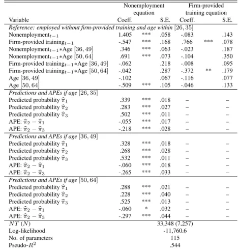
In this Section, we focus on the effect of firm-provided training on employability by allowing this effect to be heterogeneous across three age categories: 26–35, 36–49, and 50–64. The corresponding indicator variables are interacted with the lags of the nonemployment indicator and of the firm-provided training indicator. The benchmark model is augmented by these interactions and by the age indicators and re-estimated.
Table 8 reports the estimation results of the coefficients and APEs of primary interest. The coefficient of the interactions between the lag training indicator and the age categories are (jointly) not significantly different from zero. This means that firm-provided training 11These figures are available in the Eurostat webpage
http://stats.oecd.org/Index.aspx?DataSetCode=-LFS_SEXAGE_I_R.
12Empirical studies found that the Dutch reforms had a positive effect on the labour force participation of older workers (Euwals et al.,2010).
13Gielen and van Ours(2006) suggest that training of older workers in public training programs would help them to acquire new skills and to adapt to new demands, such that these workers are more likely to retain their jobs.
Table 8: Dynamic Unobserved Effects Probit Model with Age Interactions
Nonemployment Firm-provided equation training equation
Variable Coeff. S.E. Coeff. S.E.
Reference: employed without firm-provided training and age within[26,35]
Nonemploymentt−1 1.405 *** .058 -.083 .143
Firm-provided trainingt−1 -.547 *** .168 .766 *** .078
Nonemploymentt−1∗Age[36,49] .346 *** .063 -.023 .187
Nonemploymentt−1∗Age[50,64] .691 *** .073 -.104 .350
Firm-provided trainingt−1∗Age[36,49] -.062 .218 -.008 .095
Firm-provided trainingt−1∗Age[50,64] -.042 .287 -.372 ** .179
Age[36,49] -.102 .067 -.116 .077
Age[50,64] -.509 *** .105 -.046 .133
Predictions and APEs if age[26,35]
Predicted probabilityπb1 .339 *** .018 – –
Predicted probabilityπb2 .283 *** .027 – –
Predicted probabilityπb3 .502 *** .011 – –
APE:bπ2−bπ1 -.055 *** .017 – –
APE:bπ2−bπ3 -.218 *** .028 – –
Predictions and APEs if age[36,49]
Predicted probabilityπb1 .328 *** .018 – –
Predicted probabilityπb2 .268 *** .028 – –
Predicted probabilityπb3 .532 *** .011 – –
APE:bπ2−bπ1 -.060 *** .018 – –
APE:bπ2−bπ3 -.265 *** .033 – –
Predictions and APEs if age[50,64]
Predicted probabilityπb1 .288 *** .021 – – Predicted probabilityπb2 .228 *** .040 – – Predicted probabilityπb3 .525 *** .013 – – APE:bπ2−bπ1 -.060 * .032 – – APE:bπ2−bπ3 -.297 *** .044 – – N T(N) 33,348 (7,257) Log-likelihood -11,760.6 No. of parameters 115 Pseudo-R2 .544
Notes: * Significant at 10% level; ** significant at 5% level; *** significant at 1% level. All the variables included in the benchmark specification are also included here: the cor-responding estimated coefficients are not reported for the sake of brevity. The standars er-rors are robust to within-individual correlation and heteroskedasticity. The standard erer-rors of the predicted probabilities and APEs are obtained by bootstrapping the resuls 399 times (individual-cluster bootstrap with replacement).
is able to reduce the future probability of being out of the workforce for younger workers as well as for older workers. Note also that the interactions between lag non-employment status and age categories are significantly different from zero and point out that older workers not employed att−1are more like to be not employed attthan prime aged and young workers. This suggests that once older workers lose their jobs, they are less likely to find a new one. The coefficient of the indicator for older workers is instead significantly negative: older individuals are less likely to lose their jobs and therefore to be out of the workforce.
The estimation of the APEs at the sample means of the other variables confirm that firm-provided training reduces the probability of being not employed with the same mag-nitude over age classes. An employee with a given set of observed and unobserved char-acteristics and in the age range 50–64 is 6 percentage points less likely to be out of the workforce att if she had been employed with training att−1than if she had been em-ployed without training at t−1. This figure is equal to that for employees in the age range 36–49 and slightly bigger in size than that of young workers. There is evidence therefore that firm-provided training substantially increases the employability of older workers as well as the employability of young workers. Firm-provided training might be an important tool to lighten the burden of population ageing on the pension system in the Netherlands.
To some extent training is endogenous to retirement institutions. In 2006 in the public sector in the Netherlands pre-pension plans for every worker born after December 31, 1949 were abolished. To receive the same pension benefits the younger cohort has to postpone retirement for about 13 months. Montizaan et al.(2010) show that this change in future pension benefits had an effect on the expected retirement age and, through this, a positive effect on workers’ training participation. We show that this is rational to do since training leads to retaining of jobs. To retain employability of older workers age-specific subsidies to stimulate job training might be used or alternatively age-age-specific layoff taxes may be introduced.14 The first type of policy would it make it more attractive for employers to train older workers thus increasing the likelihood that they retain their employment. The second type of policy would make it more expensive for employers to fire older workers thus making it more attractive to train these workers and thereby increasing the likelihood that they retain their employability.
14Schnalzenberger and Winter-Ebmer (2009) show that an age-specific firing tax affected the labour market position of older workers in Austria. Employers had to pay a tax of up to 170% of the gross monthly income when they gave notice to a worker age 50 or more. This tax caused a substantial reduction in layoffs for older workers.
4.3
Further Robustness Checks
We perform two further sensitivity analyses to assess whether our estimates are robust to misspecification: i) due to omitting information about individuals who might have attended vocational training coursesnotprovided by the firm; ii) of the dynamics.
With regard to the former, the problem might arise as an omitted time-varying variable indicating whether the employee has undertaken training courses not provided by the firm is very likely to be correlated to the participation to a firm-provided training and, at the same time, to the future employment status. To asses whether this might be a problem, we build an indicator variableqit equal to 1 if employeeiattended vocational education
courses which were not paid or organized by the firm since the beginning of the previous year and 0 otherwise.15 The incidence of training not provided by the firm is equal to 3.5% among the employees of our sample. Firstly, we include the variable qit in the
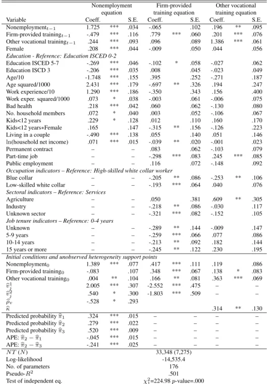
model specification as an exogenous variable and then as a predetermined variable (weak exogenous). In both cases, we find estimation results of the quantities of interest that are very much in line with those of the benchmark model. Secondly, we jointly model the process determining training not provided by the firm and the other two equations of the benchmark model, yielding the following simultanous three-equation model
yit = 1[yit−1δ1+wit−1γ1+qit−1λ1+x0itβ1+¯x0iα1+yi0θ1+wi0ψ1+qi0ϕ1+v1i+u1it>0]
wit = 1[yit−1δ2+wit−1γ2+qit−1λ2+z0itβ2+¯zi0α2+yi0θ2+wi0ψ2+qi0ϕ2+v2i+u2it>0]ifyit= 0
qit = 1[yit−1δ3+wit−1γ3+qit−1λ3+z0itβ3+¯zi0α3+yi0θ3+wi0ψ3+qi0ϕ3+κv2i+u3it>0]ifyit= 0,
whereκ is the loading factor determining, together withv2i, the points of support of the
equation of training not provided by firms. The loading factor is used to simplify the specification of the unobserved heterogeneity distribution and reduce the computational difficulty in estimating the model. The likelihood function of the benchmark model can be trivially extended to the three-equation case.
Table 9 reports the estimation results of the three-equation model. All the estimates of the nonemployment equation and of the firm-provided equation are in line with those of the benchmark model reported in Table 6. Looking at the equation for training not pro-vided by the firm, it is noted that the past employment status and the past training matter: people who were nonemployed in the past are more likely to train in the future than those who were employed without any form of training. This type of “catch-up” response is in line with the empirical evidence inMroz and Savage(2006), who found that recent unem-15The indicator for vocational training not provided by the firm is built on the basis of variables PT001, PT008, and PT017 of the ECHP data.
Table 9: Dynamic Unobserved Effects Probit Model with 3 Simultaneous Equations
Nonemployment Firm-provided Other vocational equation training equation training equation
Variable Coeff. S.E. Coeff. S.E. Coeff. S.E.
Nonemploymentt−1 1.725 *** .034 -.065 .102 .196 ** .095
Firm-provided trainingt−1 -.479 *** .116 .779 *** .060 .201 *** .076
Other vocational trainingt−1 .244 *** .093 .096 .089 1.386 *** .061
Female .208 *** .044 -.009 .050 .044 .056
Education - Reference: Education ISCED 0-2
Education ISCED 5-7 -.269 *** .046 -.102 * .058 -.027 .062 Education ISCD 3 -.206 *** .035 .008 .045 -.023 .049
Age/10 -1.748 *** .155 .395 .252 -.271 .187
Age squared/1000 2.431 *** .179 -.697 ** .326 .194 .247 Work experience/10 1.290 *** .186 -.350 .343 .156 .400 Work exper. squared/1000 .073 * .038 -.003 .061 -.006 .075
Bad health .218 *** .042 .060 .062 -.130 .080
No. household members .072 * .040 .003 .052 -.106 .067 Kids<12 years .229 * .128 .012 .110 .160 .170 Kids<12 years∗Female .165 .147 -.315 ** .156 -.126 .223 Living in a couple -.490 *** .138 .055 .140 .051 .146
ln(household net income) .071 *** .015 -.039 ** .020 -.001 .023
Permanent contract – – .083 .062 -.103 .079
Part-time job – – -.298 *** .083 .245 *** .085
Public employment – – .116 .072 -.148 .092
Occupation indicators – Reference: High-skilled white collar worker
Blue collar – – -.205 ** .086 -.253 ** .106
Low-skilled white collar – – -.193 *** .064 .040 .076
Sectoral indicators – Reference: Services
Agriculture – – .050 .381 .609 ** .305
Industry – – -.218 ** .086 -.030 .117
Unknown sector – – -.321 *** .082 -.152 .105
Job tenure indicators – Reference: 0-4 years
Unknown – – -.289 ** .144 -.009 .147
5-9 years – – -.259 *** .066 .077 .086
10-14 years – – -.213 ** .092 .182 .144
15 years or more – – -.245 ** .122 .230 .195
Initial conditions and unobserved heterogeneity support points
Nonemployment0 1.389 *** .077 .417 *** .111 .119 .086
Firm-provided training0 -.083 .107 .348 *** .067 .138 * .083
Other vocational training0 .004 ** .104 .166 ** .081 .363 *** .069 b v1 j 2.005 *** .307 -2.552 *** .475 – – b v2 j .540 * .300 -1.803 *** .509 – – b ρv -.528 * .293 b κ .314 ** .130 Predicted probabilitybπ1 .324 *** .015 – – – – Predicted probabilitybπ2 .279 *** .022 – – – – Predicted probabilitybπ3 .520 *** .009 – – – – APE:bπ2−bπ1 -.045 *** .015 – – – – APE:bπ2−bπ3 -.241 *** .025 – – – – N T(N) 33,348 (7,275) Log-likelihood -14,535.4 No. of parameters 176 Pseudo-R2 .501
Test of independent eq. χ21=224.98p-value=.000
Notes:* Significant at 10% level; ** significant at 5% level; *** significant at 1% level. Time dummies, firm size indicators, and individual time average of the time-varying covariates are included in the model specification but not reported for the sake of brevity. The standars errors are robust to within-individual correlation and heteroskedasticity. The standard errors of the predicted probabilities and APEs are obtained by bootstrapping the resuls 239 times (individual-cluster bootstrap with replacement).
ployment spells has a significant positive effect on whether a young man trains today in the US. As pointed out byMroz and Savage(2006), the “catch-up” response is predicted by the economic theory: people with a recent nonemployment spell enter the current pe-riod with a lower stock of human capital than otherwise identical individuals. When they re-enter the workforce, they dynamically re-optimize their investments in human capital and their new optimal time-path of human capital investments might lie above the one of otherwise identical individuals who did not suffer the employment shock and the loss of human capital.
Table 10: Dynamic Unobserved Effects Probit Model with Lag of Order Two
Nonemployment Firm-provided equation training equation
Variable Coeff. S.E. Coeff. S.E.
Nonemploymentt−1 1.884 *** .036 -.114 .126
Nonemploymentt−2 .769 *** .042 .154 .108
Firm-provided trainingt−1 -.466 *** .115 .760 *** .060
Predictions and APEs if the individual was employed att−2
Predicted probabilitybπ1 .232 *** .030 – –
Predicted probabilitybπ2 .172 *** .035 – –
Predicted probabilitybπ3 .533 *** .015 – –
APE:πb2−πb1 -.060 *** .016 – –
APE:πb2−πb3 -.361 *** .046 – –
Predictions and APEs if the individual was not employed att−2
Predicted probabilitybπ1 .343 *** .019 – – Predicted probabilitybπ2 .274 *** .031 – – Predicted probabilitybπ3 .688 *** .029 – – APE:πb2−πb1 -.068 *** .019 – – APE:πb2−πb3 -.414 *** .056 – – N T(N) 33,348 (7,275) Log-likelihood -8,999.0 No. of parameters 103 Pseudo-R2 .550
Notes: * Significant at 10% level; ** significant at 5% level; *** significant at 1% level. All the variables included in the benchmark specification are also included here: the corresponding estimated coefficients are not reported for the sake of brevity. The standars errors are robust to within-individual correlation and heteroskedasticity. The standard errors of the predicted probabilities and APEs are obtained by bootstrapping the resuls 399 times (individual-cluster bootstrap with replacement).
In a second sensitivity analysis, we check whether our findings are robust to the mis-specification of the dynamics. We set up a dynamic model where employment status and firm-provided training enter up to the lag of order two. We find that the lag of order two of the firm-provided training indicator does not significantly affect the nonemployment probability (p-value equal to 0.134) and thereby removed from the model specification. Table 10 reports the estimation results of the lagged variables. The sample size is now smaller: one more time period is lost as a consequence of the dynamic of higher order. A
nonemployment event att−2reinforces the positive effect of a nonemployment event at t−1on the probability of being out of the workforce at t. The estimated coefficient of lagged training is qualitatively in line with the one of the benchmark model. We estimated the APEs by conditioning on the nonemployment status att−2. In case of employment att−2, the APE of working with training att−1rather than working without training att−1is of -6 percentage points in the probability of being nonemployed (-26%). If not at work att−2, the APE is equal to -6.8 percentage points (-20%). This suggests that the estimated APEπb2−bπ1of our benchmark model is not sensitive to the dynamic spec-ification and, if any, it suffers from an upward bias. Note however that when we take the model with a dynamic of higher order, we lose observations and we restrict the analysis to individuals that are in the panel for at least four consecutive waves. This makes the as-sumption of no attrition less likely to hold. We therefore prefer to stick to the specification with a dynamic of order one.
5
Conclusions
This paper studies the relationship between on-the-job training and employability in the Netherlands. In our analysis we disentangle the true effect of training from the spuri-ous effect that might be induced by self-selection of non-random individuals into train-ing participation. We find that firm-provided traintrain-ing significantly improves employment prospects. For prime age workers who generally have a strong labour market position, in the sense that after job loss they find a new job quite easily, this relationship may be of limited interest. However, we also investigate whether for older workers training leads to higher employability. We find that older workers who receive on-the-job training are more likely to keep employment.
In many countries the labour market position of older workers is cause for concern. Older workers’ job separations are often a one-way street out of the labour force and into long-term unemployment. This is a reason for concern since demographic trends are causing an ageing of the workforce. Therefore, improving the employment position of older workers is very important from a policy point of view. Our research findings suggest that on-the-job training may be an important instrument to achieve this goal. Our research does not provide direct evidence on how to stimulate on-the-job training. Nevertheless we suggest that, in order to retain employability of older workers, age-specific subsidies to stimulate job training might be used or, alternatively, age-specific layoff taxes may be introduced. The first type of policy would make it more attractive for employers to train older workers, thus increasing the likelihood that they retain their employability. The
second type of policy would make it more expensive for employers to fire older workers, thus making it more attractive to train these workers and thereby increasing the likelihood that their employment prospects improve.
References
Alessie R, Hochguertel S, van Soest A. 2004. Ownership of stocks and mutual funds: A panel data analysis.
Review of Economics and Statistics86: 783–796.
Andrén T, Andrén D. 2006. Assessing the employment effects of vocational training using a one-factor model. Applied Economics38: 2469–2486.
Barrett A, O’Connell P. 2001. Does training generally work? The returns to in-company training.Industrial
and Labor Relations Review54: 647–662.
Bartel A. 1994. Productivity gains from the implementation of employee training programs. Industrial Relations33: 411–425.
Bartel A. 1995. Training, wage growth, and job performance: Evidence from a company database.Journal
of Labor Economics13: 401–425.
Bassi L. 1984. Estimating the effect of training programs with non-random selection.Review of Economics and Statistics66: 36–43.
Blundell R, Dearden L, Meghir C, Sianesi B. 1999. Human capital investments: The returns from education and training to the individual, the firm, and the economy.Fiscal Studies20: 1–23.
Bonnal L, Fougère D, Sérandon A. 1997. Evaluating the impact of French employment policies on individ-ual labour market histories. Review of Economic Studies64: 683–713.
Boone J, van Ours J. 2009. Bringing unemployed back to work: Effective active labor market policies.De
Economist157: 293–313.
Chamberlain G. 1984. Panel data. In Grichiles Z, Intriligator M (eds.)Handbook of Econometrics, chap-ter 22. Amschap-terdam: North Holland, 1248–1318.
Conti G. 2005. Training, productivity and wages in Italy.Labour Economics12: 557–576.
Crépon B, Ferracci M, Fougère D. 2007. Training the unemployed in France: How does it affect unem-ployment duration and recurrence? IZA Discussion Paper No. 3215, Bonn.
Dearden L, Reed H, Van Reenen J. 2006. The impact of training on productivity and wages: Evidence from British panel data. Oxford Bulletin of Economics and Statistics68: 397–421.
Euwals R, van Vuuren D, Wolthoff R. 2010. Early retirement behaviour in the Netherlands: Evidence from a policy reform.De Economist158: 209–236.
Gerfin M, Lechner M. 2002. A microeconometric evaluation of the active labour market policy in Switzer-land. Economic Jounal112: 854–893.
Gielen A, van Ours J. 2006. Age-specific cyclical effects in job reallocation and labor mobility. Labour
Economics13: 493–504.
Gritz R. 1993. The impact of training on the frequency and duration of employment.Journal of Economet-rics57: 21–51.
Ham J, LaLonde R. 1996. The effect of sample selection and initial conditions in duration models: Evidence from experimental data on training.Econometrica64: 175–205.
Heckman J. 1981. The incidental parameters problem and the problem of initial conditions in estimating a discrete time-discrete data stochastic process. In Manski C, McFadden D (eds.)Structural Analysis of
Discrete Data with Econometric Applications, chapter 4. Cambridge: MIT Press, 179–195.
Heckman J, RJ L, JA S. 1999. The economics and econometrics of active labor market programs. In OC A, D C (eds.)Handbook of Labor Economics, volume 3A, chapter 31. Amsterdam: Elsevier, 1865–2097.
Heckman J, Singer B. 1984. A method for minimizing the impact of distributional assumptions in econo-metric models for duration data. Econometrica52: 271–320.
Hyslop D. 1999. State dependence, serial correlation and heterogeneity in intertemporal labor force partic-ipation of married women. Econometrica67: 1255–1294.
Jones M, Jones R, Latreille P, Sloane P. 2009. Training, job satisfaction, and workplace performance in Britain: Evidence from WERS 2004. Labour23: 139–175.
Kluve J. 2010. The effectiveness of European active labour market programmes. Labour Economics17: 904–918.
Lalive R, van Ours J, Zweimüller F. 2008. The impact of active labour market programmes on the duration of unemployment in Switzerland.Economic Journal118: 235–257.
Lechner M, Miquel R, Wunsh C. 2008. The curse and blessing of training the unemployed in a changing economy: The case of East Germany after unification.German Economic Review8: 468–509.
Montizaan R, Corvers F, Grip AD. 2010. The effects of pension rights and retirement age on training participation: evidence from a natural experiment.Labour Economics17: 240–247.
Mroz T, Savage T. 2006. The long-term effects of youth unemployment.Journal of Human Resources41: 259–293.
Mundlak Y. 1978. On the pooling of time series and cross section data.Econometrica46: 69–85.
OECD. 2010.Employment Outlook. Paris.
Pavlopoulos D, Muffels R, Vermunt J. 2009. Training and low-pay mobility: The case of the UK and the Netherlands.Labour23: 37–59.
Picchio M. 2008. Temporary contracts and transitions to stable jobs in Italy.Labour22: 147–174.
Picchio M, van Ours J. 2011. Market imperfections and firm-sponsored training. Labour Economics18: forthcoming.
Ridder G. 1986. An event history approach to the evaluation of training, recruitment and employment programmes. Journal of Applied Econometrics1: 109–126.
Sanders J, de Grip A. 2004. Training, task flexibility and the employability of low-skilled workers.
Inter-national Journal of Manpower25: 73–89.
Schnalzenberger M, Winter-Ebmer R. 2009. Layoff tax and employment of the elderly.Labour Economics 16: 618–624.
Sianesi B. 2008. Differential effects of active labour market programs for the unemployed. Labour
Eco-nomics15: 370–399.
Stewart M. 2007. The interrelated dynamics of unemployment and low-wage employment. Journal of
Applied Econometrics22: 511–531.
van den Berg G, Lindeboom M. 1998. Attrition in panel survey data and the estimation of multi-state labor market models.Journal of Human Resources33: 458–478.
van den Berg G, Ridder G. 1994. Attrition in longitudinal panel data and the empirical analysis of dynamic labour market behaviour. Journal of Applied Econometrics9: 421–435.
Wooldridge J. 2005. Simple solutions to the initial conditions problem in dynamic, nonlinear panel data models with unobserved heterogeneity.Journal of Applied Econometrics20: 39–54.