Exploring the Quasar Luminosity Function with Quasars Selected by both Color and Variability

(1)

with Quasars Selected by both Color and Variability

A Thesis

Submitted to the Faculty

of

Drexel University

by

Christina M. Peters

in partial fulfillment of the

requirements for the degree

of

Doctor of Philosophy

(2)

This work is licensed under the terms of the Creative Commons Attribution-ShareAlike license Version 3.0. The license is available at

(3)

Acknowledgments

First, I would like to express my sincere gratitude to my advisor Gordon Richards for his continuous

support of my research. His guidance, patience, and motivation have helped me immensely in my

Ph.D. work and I couldn’t have asked for a better mentor.

To the rest of my thesis committee: Beth Willman, Luis Cruz Cruz, Michael Vogeley, and Steve

McMillan, I offer my sincere appreciation for the insightful comments and encouragement they

provided.

This research could not have been accomplished without my fellow graduate students. Thank you

for the stimulating discussions, bug checking line after line of code, and many coffee trips.

I will always be very grateful to Saint Thomas Aquinas Catholic Community, my incredibly

support-ive South Philadelphia home. Your encouragement when the times got rough is much appreciated.

Many thanks to my cycling teammates for all of the long rides and fast sprints that helped me stay

balanced while writing this thesis.

Finally, to my parents and my brother for supporting me throughout my many years in school. My

(4)

List of Tables

2.1 Master Quasar Catalog . . . 12

3.1 NBC KDE Results - Self Test Non-quasar and Quasar Fraction . . . 30

3.2 NBC KDE Results: Self Test Completeness and Efficiency . . . 30

3.3 NBC KDE Results: Test Set Classification of Spectroscopically Confirmed Quasars . . 40

4.1 Redshift Estimate Statistics . . . 51

4.2 Smoothing Parameters for Redshift Probability Distributions . . . 57

4.3 Simulated Survey Datasets from the LSST Operations Simulator (OpSim) . . . 65

5.1 Quasar Candidates . . . 69

6.1 SED Groups . . . 86

(7)

List of Figures

2.1 Distribution of quasars and non-quasars in two SDSS color spaces from the coadded photometric catalog (Annis et al., 2014). Non-quasars (orange contours), such as stars and compact galaxies, are considered contaminants when trying to accurately classify quasars (cool colors). Notice the overlap of non-quasars in the region in which mid-redshift quasars (2.2< z <3.5; dark blue contours and scatter points) lie. This overlap makes it difficult to accurately classify an object in this region as a quasar or non-quasar, and motivates searches for alternative methods of classification, like variability. Quasars in three redshift ranges are shown: low-redshift (z < 2.2; green contours and scatter points), mid-redshift, and high-redshift (z >3.5; light blue dots). The extension of the non-quasar color space atg₋r_∼1.4 is not real, but an artifact of including objects with largeu-band photometric errors (and thus spilling into the true quasar parameter space). 14 2.2 g and u-band light curves (left panel) and g-band structure function fit with a power

law model (right panel) of SDSS J013417.81-005036.2, a redshift 2.26 quasar from SDSS Stripe 82 (also shown in Figure 4.5). This quasar is shown as an example representative of the data set. Left panel: There are 126 total observations in the g-band; 106 of those meet the PSF-width and airmass requirements (green points with error bars), while those that were removed are shown in orange. The dark green dashed line is the running median (with a window of 50 days and steps of 5 days) calculated from theg-band observations. Theu-band observations are similarly shown in blue and red. Right panel: The pairs of photometric points from the g-band light curve in the left panel are shown as a hex-bin density plot where the darkness of the hex bin indicates the number of points in that bin. The power law fit is shown as a green line. The method for calculating the structure function and the equation used to fit the structure function are detailed in Section 2.4. In the case of this object, the fitting algorithm gives Ag = 0.105 and γg = 0.102. The

points removed as outliers in the left panel would only contribute|∆m_|>0.25 mag values. 16 2.3 Quasar and non-quasar data sets in variability parameter space for the g-band

observa-tions. Note that, unlike in the color-color plots in Figure 2.1, there are no distinct changes in the variability features as a function of quasar redshift in this parameter space. This is advantageous because it allows separation of the quasars from the non-quasars in the variability space without extreme changes in completeness at specific redshifts, as seen with color selection. Non-quasars, such as stars and normal galaxies, are shown in or-ange contours. Quasars are shown in cool colors as three redshift regions: low-redshift (z < 2.2; green contours and scatter points), mid-redshift (2.2 < z < 3.5; dark blue contours and scatter points), and high-redshift (z >3.5; light blue dots). . . 21 2.4 All spectroscopically confirmed quasars shown in A vs. γ space in each of the SDSS

bands, colored by redshift. This figure demonstrates the difficulty involved in combining the observations in all five bands to obtain one light curve and one structure function in order to describe the overall variability without previously knowing the object’s redshift. Note how the distribution of points shifts with band and with redshift. In particular, A

andγvalues agree well in theg,r, andiband, but the large photometric errors inuand

(8)

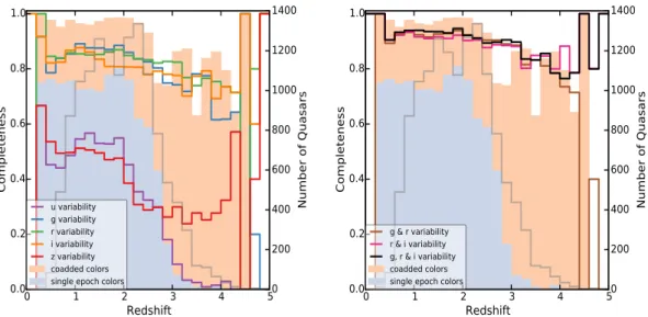
3.1 Fraction of quasars correctly classified as quasars (completeness). These panels demon-strate that quasars can be separated from non-quasars in the variability space without extreme changes in completeness at specific redshifts. In both panels the gray line shows the number of quasars in each bin (right axis) and light blue (single epoch) and peach (coadded epochs) histograms show the completeness of color-only selection (left axis, Sec-tion 3.3.1). Note the catastrophic loss of high-zquasars from single-epoch colors and the incompleteness atz_∼2.8 even for coadded colors. Also showm is classification from vari-ability only: single bands (left panel) and combinations of multiple bands (right panel). The g, r, and i bands are shown as blue, green, and orange lines respectively. There are no dramatic drops in theg₋,r₋, ori₋bands variability at distinct redshifts, just a gradual decline with increasing redshift, which is related to observed magnitude, signal to noise ratio, and time scale of variability in the observer’s frame. The overall completeness using variability alone is not as high as coadded colors alone at low redshifts, but is more successful than single-epoch colors alone at high redshifts. . . 31

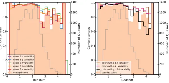
3.2 Fraction of quasars correctly classified as quasars using coadded colors and variability, as a function of redshift. Notice the improved completeness near redshifts 2.7 and 3.5, where the quasars and non-quasars overlap in color space, with the addition of variability features. Shown are single bands of variability combined with coadded colors (left panel) and combinations of multiple bands of variability combined with coadded colors (right

panel). In both panels the gray line shows the number of quasars in each bin (right axis). 32

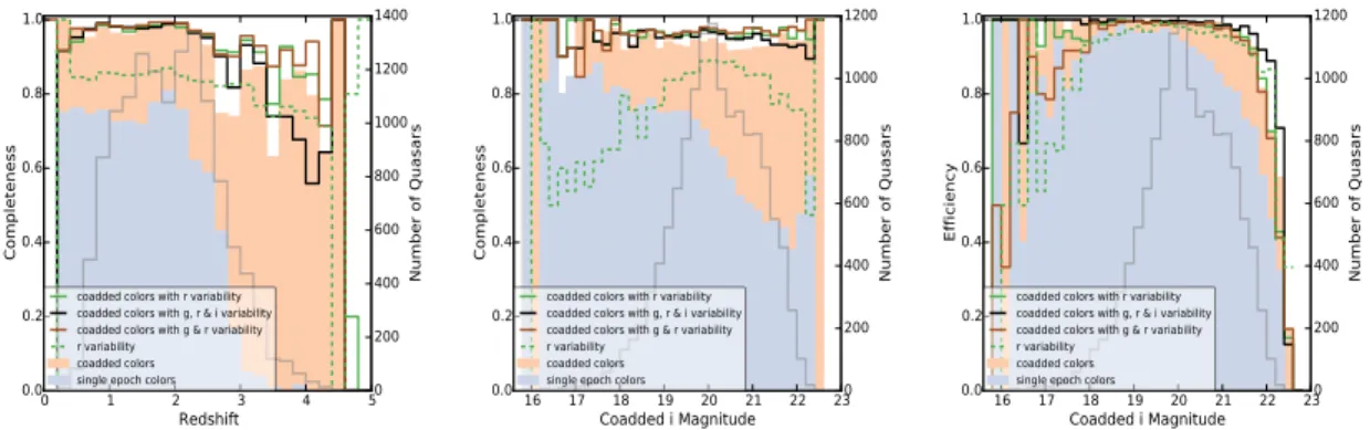
3.3 Comparison of self tests using with different combinations of color and variability. These panels demonstrate that the combination of color and variability gives the best results for completeness and efficiency as a function of redshift and magnitude with more details in the text. Shown are the completeness (known quasars classified as quasars divided by known quasars) as a function of redshift (left panel), completeness as a function of coadded i-band magnitude (center panel), and efficiency (known quasars classified as quasars divided all objects classified as quasars) as a function of coadded i-band magnitude (right panel). The gray line shows the number of quasars in each bin (right axis). . . 33

3.4 Color and variability parameter space plots showing the results of test set classification using a single quasar training set covering the full quasar redshift range (Section 3.4.1). These panels demonstrate that the incorrectly classified quasars lie in the area where quasars and non-quasars overlap in color and variability space and that the candidate quasars closely mirror the distribution of the known quasars and extend slightly beyond in the parameter space (including a region known to be inhabited by white dwarfs in the blue corner of the upper right panel). Colors left panel: u₋g color vs.g₋r,colors

right panel: g₋r vs.r₋i, variability left panel: Ag vs. γg, and variability right panel:

Ar vs.γr. Objects in the test set classified as non-quasars are shown as gray contours,

quasar candidates that are not spectroscopically identified are shown as green contours and scatter points for outliers, spectroscopically identified quasars classified as quasars are shown as orange contours and scatter points for outliers, and spectroscopically identified quasars incorrectly classified as non-quasars are shown as purple dots. The red dashed line in the upper right panel is the white dwarf cut described in Eq. 5.3. Levels for contours in Figures 3.4 and 3.7: gray: colors - 95%, 90%, 80%, 60%, 40%, 20%, variability - 98%, 95%, 90%, 80%; green: colors - 90%, 80%, 60%, 40%, 20%, variability - 90%, 80%, 60%; orange: 90%, 80%, 60%, 40%, 20%. . . 36

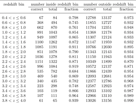
3.5 Classification of a test set of quasars with known spectroscopic redshifts, using the train-ing sets divided into redshift bins. Dark blue indicates all quasars in that bin, light blue indicates quasars classified with the correct redshift. The ratio of the two is the completeness of quasars inside the redshift bin. . . 38

(9)

3.6 Comparison of spectroscopic redshift to the bin into which known quasars were classified with the highest probability. Left panel: Spectroscopic redshift vs. the most probable redshift bin. Right panel: Histogram of ∆z (the most probable redshift bin minus the spectroscopic redshift). Only 5.6% of the quasars have|∆z_|>0.5 . . . 38 3.7 As Figure 3.4, color and variability space plots showing the results of test set classification,

but using redshift bins (described in Section 3.4.2). In the bottom panels, the selection in variability parameter space shows no noticeable difference to Figure 3.4, which is not surprising as Ag vs.γg andAr vs.γr have no strong redshift trends. However, there are

slight differences in color space (top panels). This is discussed further in Section 5.1. . . 39

4.1 The SDSS filter curves (u- purple,g- green,r- light green,i- orange, andz- red) shown with the Vanden Berk et al. (2001) SDSS composite quasar spectrum at four different redshifts. . . 42

4.2 The effective wavelength of each of the SDSS filters as a function of the composite quasar spectrum’s redshift. The dashed line in each panel is the nominal effective wavelengths of the SDSS bandpasses for a flat-spectrum source (3551, 4686, 6165, 7481, and 8931 ˚A). 43

4.3 The difference between the angular deflection of an incoming photon for the composite quasar spectra and the pipeline correction in each of the SDSS filters. Shown for four different airmasses: 1.00 (solid grey line, no offset because this is at the zenith), 1.10 (dotted line), 1.25 (dashed line), and 1.40 (solid colored line). . . 44

4.4 Tangent of the zenith angle (Z) vs. offset in position along the parallactic angle in the

u-band [left] and g-band [right] for quasars at a range of redshifts. This shows multiple epochs of observations at different airmasses (where airmass _∼secZ). . . 46 4.5 The measured astrometric offset along the parallactic angle as a function of tan(Z).

Shown is SDSS J013417.81-005036.2, a redshift 2.26 quasar from SDSS Stripe 82, the same object shown in Figure 2.2. This quasar is shown as an example that is representative of the data set. Each point refers to a different observation of this object, at a different airmass. The astrometric accuracy is ∼0.03 arcsecs forg <20.0, but up to 0.1 arcsecs for g _∼ 22.0 (Pier et al., 2003). u-band observations are shown in blue; those points that were outliers removed from the light curve in Figure 2.2 are shown in red. g-band observations are shown in green, with outliers removed from the light curve shown in orange. The fits, shown as solid blue and green lines, have an y-axis intercept of zero. For this quasar, the slope of the line (offset along the parallactic angle) in the u-band (auP ar) is -0.055 andg-band (agP ar) is 0.105. The astrometric redshift is found to be 2.57. . . 47

4.6 Slope of the line (offset along the parallactic angle) with respect to redshift in theu-band (auP ar) andg-band (agP ar) as a function of redshift for the quasar sample (left panel) and as a function of magnitude for non-quasars (right panel). Left panel: While the changes in these astrometric parameters are not as strong as the changes in color with redshift, they provide another source of redshift information. Right panel: The differences between the distributions in the left panel and right panel can aid in the separation of quasars from non-quasars. For example, objects with large negative values ofauP arare more likely to be non-quasars than quasars. . . 48

(10)

4.7 Spectroscopic redshift vs. photometric redshift in hex bins with logarithmic gray scale, using (top left panel) optical colors (both single epoch and coadded, when available), (top

right panel) astrometry as described in Section 4.1, (bottom left panel) optical and NIR

adjacent colors, and (bottom right panel) combined optical and astrometry as described in Section 4.4. This illustrates those redshifts where the algorithm has the largest error rate (either due to degeneracy between distinct redshifts or smearing of nearby redshifts). 52

4.8 Histogram of the difference between spectroscopic redshift and estimated redshift. Note how the distribution tightens toward ∆z = 0.0 from the SDSS color photometric redshifts to the astro-photometric redshifts. Shown are optical colors (green), combined optical and astrometry as described in Section 4.4 (purple), and optical and NIR adjacent colors (orange). Shown in solid black is the histogram of classification in redshift bins from Figure 3.6. . . 53

4.9 Truth set of quasars divided into six bins to determine optimal smoothing. The bins were chosen empirically based on the shape of the photometric redshift PDFs which are shown in the following Figure. . . 55

4.10 Photometric redshift PDFs for 100 randomly of quasars from each of the bins shown in the preceding figure. The vertical gray line is the spectroscopic redshift of each quasar. The y-axis scale in each subplot is identical. The bins were chosen empirically to have quasars with PDFs of similar shapes. . . 56

4.11 Representative quasars from each of the bins to demonstrate optimal smoothing of the photometric and astrometric redshift PDFs. The green lines indicate the original and smoothed photometric redshift PDF. The vertical green line is the peak of the smoothed PDF. The astrometric PDF is similarly shown in purple. The product of the PDFs is shown in red, with the peak indicated by a vertical line. The spectroscopic redshift is shown as a vertical black line. . . 58

4.12 Optimal smoothing of the photometric redshift [x-axis] and astrometric redshift [y-axis] PDFs for each of the bins. The minimum value of ∆z is indicated as a white dot and this value ofσphotandσastromis used for all quasars in that bin. . . 59

4.13 Spectroscopic redshift vs. photometric redshift shown in orange under spectroscopic red-shift vs. astro-photometric redred-shift shown in gray. . . 60

4.14 Normalized histogram of spectroscopic redshift in panels based on bins of photometric redshift from 0.3 to 5.0 in the same bins as the luminosity function in Section 6.2. These panels demonstrate which photometric redshift ranges are most unreliable and most reli-able. Photometric redshifts were calculated using SDSS colors (green), SDSS colors and astrometry (purple), and SDSS and VHS colors (orange). In particular, note the bimodal distribution at 0.68< zphot<1.06 compared to the precision at 1.06< zphot<1.44 and

3.0 < zphot < 3.5. This bimodality is caused by degeneracies in color-redshift space.

Systematics in photometric redshift errors are corrected when calculating the quasar luminosity function in Section 6.2 . . . 62

4.15 Example linear fits of the measured astrometric offset along the parallactic angle as a function of tan(Z) forz = 0.8 and 2.2 quasars in theu-band [left] andz = 0.4 and 0.8 quasars in the g-band with 20 observations from airmass 1.0 to 1.95. Error bars are 20 mas. The semi-transparent lines illustrate the fits from various MCMC ensemble walkers. 64

(11)

4.16 The distribution of fits from the MCMC forz= 0.8 and 2.2 quasars in theu-band [left] andz= 0.4 and 0.8 quasars in theg-band [right]. The K-S statistic and p-values indicate that the quasars at these redshifts could be distinguished using DCR alone with enough observations. . . 64

4.17 Sky map of the p-value comparingz= 0.4 and 0.8 ing-band with an airmass limit of 1.3 after 1 year [left], with an airmass limit of 2.0 after 1 year [center], and with an airmass limit of 1.3 after the full survey [right]. The sky map has a resolution of_∼27.5 arcmin. 65 4.18 Max airmass [left column], number of observations [center column], and p-value forz=

1.0 and 1.4 quasars [right column] for the baseline cadence in theu-band after one year [top row],g-band after one year [middle row], andg-band after survey completion [bottom row]. Sky map has a resolution of_∼27.5 arcmin. . . 67 5.1 Stacked histogram of redshift for known Stripe 82 quasars and new quasar candidates.

Left panel shows the quasars and candidates i < 19.9 and right panel shows i > 19.9.

Spectroscopic quasars found as quasar candidates and spectroscopic quasars missed are both binned by spectroscopic redshift. Quasar candidates found by both methods and quasar candidates found only using a binned quasar training set are both binned by where the candidate was classified with the highest probability. These bins only span 0.4 < z < 4.0. Quasar candidates found only using a quasar training set over the full redshift range are binned by the astro-photometric redshift. . . 72

5.2 Histogram of coadded i band magnitude for known Stripe 82 quasars and new quasar candidates. In purple are the previously known, spectroscopically confirmed quasars returned by the selection. The quasar candidates returned by the selection are shown in orange and the new quasar candidates are shown in green. . . 73

5.3 Ar vs. γr for the training sets (left panel) and test set (right panel) shown with the

Schmidt et al. (2010) variability selection cuts (Equations 5.4 - 5.6) as gray lines. Left

panel: Orange contours show the non-quasar training set and purple contours and scatter

points show the quasar training set. Right panel: Gray contours show all objects in the test set classified as non-quasars and green contours and scatter points show all objects in the test set classified as quasars. . . 74

6.1 Left panel: Ratio of MQC quasars returned by classification (using a training set over the

full redshift range) to all those in the MQC on Stripe 82. This ratio allows for a correction due objects with too few observations to calculate variability features, the exclusion of extended sources, and incompleteness in the selection algorithm. The fraction is given as a function of coaddedi-band magnitude for two redshift ranges. Right panel: Quasar number counts as a function of redshift and i-band magnitude. Black points give the spectroscopic number counts reported in Richards et al. (2009a); circles forz <2.2 and triangles for 3< z <5. The open purple and green squares give the raw number counts (with Poisson error bars) for the candidates reported here. The filled colored squares give the number counts corrected using the left panel. The vertical dashed red line at

(12)

6.2 Corrections and cuts used in the QLF in Figure 6.3. Left panel: Completeness fraction, in bins of redshift and absolute magnitude,Mi[z= 2], for candidate selection. Similar to

Figure 6.1left panel, but in two dimensions. The number of quasars with spectroscopic redshifts on Stripe 82, even if they were excluded from the training set and test set, was divided by all quasars with spectroscopic redshifts that were recovered as candidate quasars. This is to correct for incompleteness from too few observations to calculate variability features, the exclusion of extended sources, and incompleteness in the classi-fication algorithm. Center panel: Completeness fraction for astro-photometric redshifts. All of the training set quasars are binned by spectroscopic redshift (purple) and astro-photometric redshifts (green). The ratio of the two is shown in grey (right axis). The astro-photometric redshifts of the candidate quasars, after being corrected by the com-pleteness fraction and assuming that objects without spectroscopic redshifts have the same astro-photometric redshift errors as those with spectroscopic redshifts, are shown in purple. Right panel: Astro-photometric redshift vs. absolute magnitude,Mi[z= 2], of

all quasar candidates. The green line shows the brightness limit for bins that are used in computing the luminosity function. Purple curves show the i= 15.0, 19.1, and 21.0 magnitude limits. . . 79

6.3 Mi[z= 2] binned luminosity function of the sample with astro-photometric redshifts using

the method from Page & Carrera (2000) (with Poisson error bars). The mean redshift of each slice is given in each panel. Black filled circles are complete bins, empty triangles indicate the lower limit for complete bins where the completeness fraction (shown in Figure 6.2 left panel) is 0, and empty circles are partial bins (a portion of the bin is dimmer than i = 22). The grey circles show the binned luminosity function and the grey dashed line shows the z = 2.01 curve both from Richards et al. (2006, Figure 18) for comparison. In the z = 2.4, 2.8, and 3.25 panels, the red squares show the binned luminosity function for BOSS quasars from DR9 from Ross et al. (2013, Figure 11). In the 4.75 panel, the green squares, purple squares, and dashed black line show the binned luminosity function at z = 4.9 for Stripe 82, DR7, and double power law fits from the maximum likelihood analysis from McGreer et al. (2013, Figure 12 and Figure 13). . . . 81

6.4 Distribution of the weights for the first three components (W1, W2, and W3) for the

quasar spectra (left panel) and the distribution at left normalized after dividing by the component mean (right panel). These differences are small, but they are crucial for making sure that all of the objects are calibrated in the same way. . . 84

6.5 Distribution of the weights for the first three components (W1, W2, and W3) for the

quasar spectra as function of redshift. Shown with the best fit line used for dividing the quasars into groups. . . 85

6.6 The three groups shown as a function of CIV blueshift and equivalent width. The division inW1-W2-W3space separated the quasars in this space with no CIV information used

in the ICA analysis. . . 85

6.7 The three groups as a function of redshift (left panel) and magnitude (right panel). Note that there is a strong difference in the selection function between the Hard and Soft SED groups. . . 86

(13)

6.8 Top panel: Spectroscopic redshift vs. absolute magnitude,Mi[z= 2], of all quasar

candi-dates. The green line shows the brightness limit for bins that are used in computing the luminosity function. Purple curves show the i= 15.0, 19.1, and 21.0 magnitude limits.

Bottom panel: Mi[z = 2] binned luminosity function of the full population (black) and

the three equal sized clusters (with Poisson error bars). The mean redshift of each slice is given in each panel. Black filled circles are complete bins, empty triangles indicate the lower limit for complete bins where the completeness fraction is 0, and empty circles are partial bins (a portion of the bin is dimmer than the brightness limit). The colored points are scaled by the number quasars in the group and all points corrected based on the selection function. . . 87

6.9 Top panel: Spectroscopic redshift vs. absolute magnitude,Mi[z= 2], of all quasar

candi-dates. The green line shows the brightness limit for bins that are used in computing the luminosity function. Purple curves show the i= 15.0, 19.1, and 21.0 magnitude limits.

Bottom panel: Mi[z = 2] binned luminosity function of the full population (black) and

the three equal sized clusters (with Poisson error bars). The mean magnitude of each slice is given in each panel. Black filled circles are complete bins, empty triangles indicate the lower limit for complete bins where the completeness fraction is 0, and empty circles are partial bins (a portion of the bin is dimmer than the brightness limit). The colored points are scaled by the number quasars in the group and all points corrected based on the selection function. . . 89

7.1 Normalized photometric redshift PDFs (top panel) and absolute magnitude as function of photometric redshift (bottom panel). The darkness of the line indicates the redshift probability (vertical axis of the top plot). The spectroscopic redshifts for each object are shown as purple points and the peak of the photometric redshift are shown as green points. Note how the gray gradient matches the widths of the spectroscopic redshifts more closely than the photometric peaks, which suggests that this analysis can be improved by using the full PDF of the photometric redshift instead of the peak value. . . 95

(14)

Abstract

Exploring the Quasar Luminosity Function with Quasars Selected by both Color and Variability

Christina M. Peters Gordon T. Richards Ph.D.

A non-parametric Bayesian classification selection algorithm was used to demonstrate that a

combination of optical colors and variability features improves quasar classification efficiency and

completeness over the use of colors alone, suggesting that this is a good set of features to use in

classi-fication algorithms for future time-domain focused sky surveys. These features were used to identify

35,820 type 1 quasar candidates in a 239 deg2 field of the Sloan Digital Sky Survey (SDSS) Stripe

82. Color analysis was performed on 5-band single- and multi-epoch SDSS optical photometry and

variability parameters were calculated by fitting the structure function of each object in each band

with a power law model. Using variability alone, colors alone, and combining variability and colors,

quasar completeness of 91%, 93%, and 97% and efficiency of 98%, 98%, and 97%, respectively, was

achieved. Particular improvement was seen in the selection of quasars at 2.7< z <3.5 where quasars and stars have similar optical colors. Of the 22,867 quasar candidates that are not spectroscopically

confirmed, 95.7% are dimmer than coaddedi-band magnitude of 19.9, the cut off for spectroscopic follow-up on Stripe 82. Brighter than 19.9, 5.7% more quasar candidates were found without

con-firming spectra in sky regions otherwise considered complete. In addition to calculating empirical

optical photometric redshifts for all candidate quasars, astrometric redshifts were calculated using

parameters determined by measuring the differential chromatic refraction (DCR) effect with the

purpose of breaking degeneracies in the photometric redshifts. The combined astro-photometric

redshifts are more accurate than optical and near-infrared photometric redshifts. Potential

obser-vation schedules for the Large Synoptic Survey Telescope (LSST) were analyzed to determine how

well quasars of different redshifts can be distinguished using the DCR effect. The resulting quasar

sample has sufficient purity (and statistically correctable incompleteness) to produce a luminosity

(15)

and redshift estimation. The quasar luminosity function of a uniformly-selected spectroscopic quasar

sample, grouped according to emission-line properties, suggests that the space density of quasars

with different underlying spectral energy distributions (SEDs) has evolved differently with redshift,

(16)

(17)

Chapter 1: Introduction

In this work I describe a suite of methods that uses multi-epoch photometry to identify a large

number of quasars, determine their redshift, and study their evolution with redshift and luminosity

without the need of spectroscopy. First, I identify quasars using optical photometry, by

simultane-ously using the distinctive and quantifiable features of color and variability to distinguish quasars

from other types of objects in the sky. As a proof of concept for this method, I classify the objects

in the Sloan Digital Sky Survey (SDSS) Stripe 82 where about 100 repeat observations have been

performed, allowing for study of variability. I identify 35,820 quasar candidates, 63% of which had

not been previously identified. Then, to ensure that the sample is useful for doing science, I have

used a sophisticated statistical method to calculate a photometric redshift (i.e. distance estimate)

based on imaging alone for each of the quasar candidates. To improve upon traditional

photomet-ric redshifts methodologies, I incorporate astrometphotomet-ric information into my calculations, using the

prismatic effects of the Earth’s atmosphere as a low-resolution spectrograph. I discuss how this

can be beneficial in redshift estimates for future large photometric surveys. Finally, I construct the

quasar luminosity function (QLF), which measures the space density of quasars per unit luminosity

and redshift. I compare the redshift evolution of the photometric sample to previous spectroscopic

quasar samples and populations of quasars with different underlying spectral energy distributions

(SEDs).

In 1960, Thomas Matthews and Allan Sandage were searching for the optical counterpart to

a radio source and found a variable point source object whose spectrum had broad emission lines

that did not correspond to any known element or molecule (Matthews & Sandage 1963; Greenstein

& Matthews 1963). Several similar sources were later found, and they were named quasi-stellar

objects (QSOs) or quasars. Later that year, the pattern of emission lines in the quasar spectra

(18)

These strange new objects were found to be the most distant objects in the Universe; so far away

that in images the galaxy is not visible just the bright active galactic nucleus (AGN). To be visible

at such distances quasars must be very powerful sources of energy, in fact, they produce _∼105 _as

much energy as the Milky Way and are visible out to redshifts_∼6.

Since their discovery, quasars have been identified by their colors, variability, and (lack of)

proper motion—but not through all of these methods combined. The standard way of identifying

large numbers of candidate quasars is to make “color cuts” using optical (or infrared) photometry

(e.g., Richards et al. 2002; Croom et al. 2004; Warren et al. 2000; Lacy et al. 2004; Stern et al.

2005; Maddox et al. 2012; Assef et al. 2013). This is because the majority of unobscured quasars at

z <2.5 are much bluer than the majority of stars in the optical and are much redder in the infrared. However, this process is neither complete (identifying all true quasars) nor efficient (minimizing false

positives). Such methods do an effective job of identifying a large number of interesting objects with

relatively little effort; however, better methods are needed to scale to future surveys to allow for

scientific analysis without the need for spectroscopic confirmation.

In addition to classification by color, time-domain data make variability a promising way for

classifying objects. The long history of such work can be followed through Koo et al. (1986), Hughes

et al. (1992), Vanden Berk et al. (2004), de Vries et al. (2005), Sesar et al. (2007), Kelly et al. (2009),

Koz lowski et al. (2010), Schmidt et al. (2010), Butler & Bloom (2011), MacLeod et al. (2010, 2011,

and 2012), and Graham et al. (2014). Specifically, quasars exhibit stochastic, aperiodic variability

with variations of order 10% on the timescale of years (de Vries et al. 2003; Vanden Berk et al. 2004).

The amplitude and time scale of this variability are sufficiently distinctive to allow one to identify

an object as a candidate quasar.

Many current and future astronomical imaging surveys (SkyMapper: Keller et al. 2007;

Palo-mar Transient Factory: Law et al. 2009; Pan-STARRS: Stepp et al. 2010; DES: The Dark Energy

Survey Collaboration 2005; LSST: Ivezi´c et al. 2008) are focusing on time-domain astronomy and in

anticipation, it is important to determine the effectiveness of classification using variability

(19)

selection will fill in the gaps in color selection methods (or replace color selection entirely). Indeed,

investigations such as Schmidt et al. (2010), MacLeod et al. (2011), and Butler & Bloom (2011)

have been quite successful. However, variability-only selection suffers from its own set of problems.

For example, high-redshift quasars can be lost when using a fixed observed-frame variability

analy-sis: Lyαabsorption reduces the quasar continuum in blue bands and the redder bands have larger photometric errors for fainter objects. In addition, variability increases with lower luminosity (e.g.,

Vanden Berk et al. 2004), but so does the host galaxy contribution—potentially complicating the

selection of such objects without careful difference imaging to remove the host galaxy

contribu-tion. Thus, it is important to investigate how well variability selection works by itself versus being

combined with other methods (e.g., colors and astrometry).

The first part of this project is to simultaneously use the distinctive and quantifiable

charac-teristics of color and variability to distinguish quasars from stars and inactive galaxies. The Sloan

Digital Sky Survey (SDSS; York et al. 2000) repeatedly imaged a 2.5◦ _{equatorial section of the sky}

referred to as Stripe 821_{(Abazajian et al. 2009; Annis et al. 2014; Jiang et al. 2014). The light curves}

of spectroscopically confirmed quasars and stars from Stripe 82 give us the information needed to

develop and test classification of quasars.

Specifically, color and variability data are used in combination with modern machine learning

techniques to uncover previously unidentified quasars in the SDSS Stripe 82 region and to pave the

way for improved multi-faceted selection in the future. The goal is not necessarily to produce the

most complete or efficient catalog possible but to test the combined use of colors and variability data

in classification. In this investigation, some simplifications are made to the process that could be

explored in more detail in future work. Specifically, this analysis is focuses on point sources to avoid

the problem of the host galaxy washing out the variable nucleus (reducing our sensitivity to

low-redshift quasars), a simple power-law model of variability is used as opposed to more sophisticated

(but not necessarily “correct”) models such as the damped random walk, variability data from each

band is used separately instead of merging them together, and a simplistic approach is taken to

(20)

combine photometric redshift information from different methods. Each of these simplifications is

worthy of a separate investigation to determine precisely how much they affect this classification.

A shortcoming of the traditional quasar identification process is that it usually involves selecting

quasar candidates by identifying them as outliers using cutsin the observed data space(e.g., selecting

all point sources withu₋g <0.6). My classification instead makessimultaneoususe of all of the data types available and uses modern statistical techniques (based on kernel density estimation; KDE) to

make cuts inprobability space(e.g., objects with an expected quasar probability greater than 50%).

The methods developed by my research group (Richards et al. 2004; Riegel et al. 2008;Richards et al.

2009a; Richards et al. 2009b) and others (e.g., Suchkov et al. 2005; Ball et al. 2006; Davoodi et al.

2006; Gao et al. 2008; Bailer-Jones et al. 2008; D’Abrusco et al. 2009; Guy et al. 2010; Schmidt et al.

2010; Abraham et al. 2012; Bovy et al. 2012; Peng et al. 2012; Gupta et al. 2014) are extended to

create a classification algorithm for time-domain focused sky surveys. While this approach has been

shown to work well in the past (e.g., Richards et al., 2004, 2009a), future work will inevitably explore

other modern statistical techniques such as described by Feigelson & Babu (2012) and references

therein.

The quasar candidates that result from the application of this method are only identified

photo-metrically; they lack spectroscopy which not only would confirm the type of an object, it crucially

also would determine the redshift. Most galaxy and cosmology science requires objects with verified

types and redshifts. Even with the upcoming large spectroscopic surveys, e.g. the Dark Energy

Spectroscopic Instrument2 _{(DESI; Levi et al. 2013) and Subaru Prime Focus Spectrograph}3 _(PFS;

Takada et al. 2014), there is not enough follow-up for even a small fraction of the sources that current

photometric surveys will see. Thus, it will be critical to have an alternative to the current practice

of following up on each object to have an accurate redshift.

When calculating photometric redshifts for galaxies, the standard is to fit a suite of spectral

templates to the flux information from the images. When the process fails, it is because there is

some level of degeneracy in the suite of templates. Additionally, the galaxy population has multiple

2_desi.lbl.gov 3_{sumire.ipmu.jp}

(21)

sub-populations and inherent scatter because not all galaxies of the same type are identical. More

complicated are the galaxies which contain a bright central region caused by an AGN. There are

many sophisticated methods for estimating photometric redshifts (e.g. Rowan-Robinson et al. 2008;

Salvato et al. 2009). Quasar photometric redshifts based on templates have not been shown to work

well, particularly when the AGN component is brighter than the host galaxy component (Assef et al.,

2010). However, empirically based algorithms have been successful. These algorithms essentially

least-squares fit between the candidate quasar colors and the mean colors of quasars as a function

of redshift. In this work the algorithm described in Richards et al. (2001) and Weinstein et al.

(2004) is used, which ranks among the most accurate for (luminous) quasar photometric redshift

estimates. This algorithm, in addition to identifying a most probable redshift, generates a probability

distribution for a continuum of redshifts.

I improve this process further by using the effective prismatic effects of the Earth’s atmosphere as

a low-resolution spectrograph (Kaczmarczik et al., 2009). In short, the apparent positions of quasars,

with their strong emission features, is a function of the pass band and redshift. This behavior of

quasars allows me to uniquely incorporate astrometric information into the photometric redshift

estimates.

As demonstrated in Figure 9 of Kaczmarczik et al. (2009), the astrometric redshift and the

photometric redshift probability distribution functions (PDFs) contain complementary information

about the quasar redshift. The photometric redshifts are more accurate in general, but have

de-generacies, particularly at redshifts 0.4 and 2.0 (Richards et al., 2001). The astrometric redshifts,

when combined, can break these degeneracies. The PDFs are optimally combined by giving them

a relative weighting based on the shape of the photometric redshift PDF. This weighting is done

by smoothing the PDFs before multiplying them. The improvements of these astro-photometric

redshifts are comparable to those from adding infrared detections to the photometric redshifts.

This work provides a stepping stone for quasar classification for future surveys such as the Large

Synoptic Survey Telescope4 _{(LSST). Eventually, each region of LSST will be imaged about 200} 4_lsst.org

(22)

times in each filter over the ten years of the survey, allowing for the study of the variability on

scales of minutes to a decade. This focus on time-domain astronomy is an exciting new era in

surveys, but the lack of spectroscopy creates a problem for confirming the type of an object. As the

number of spectroscopic fibers allocated to quasar identification pales in comparison to the number

of photometrically detected objects that merit spectroscopic follow-up, it is only through complete

and efficient object classification coupled with accurate redshift estimates that we can overcome

the lack of spectroscopy in LSST and other future astronomical surveys and maximize their science

output.

The LSST Operations Simulator (OpSim) and Metric Analysis Framework (MAF) make it

pos-sible to determine how effective the telescope and processing pipeline will be at reaching the various

science objectives of the telescope. Multiple OpSims have been produced by the LSST Collaboration

with deviations from the current baseline cadence for the survey. The MAF software package allows

interested parties to interact with the OpSims to determine how well a given cadence will allow them

to do their science with the future LSST data. In this work, I present a MAF to evaluate how well

LSST will be able to constrain quasar redshifts using astrometric data alone.

Identification of large numbers of quasars/AGNs over a broad range of redshift and luminosity

is crucial for many scientific endeavors. Work that requires a greater density of objects than current

spectroscopic surveys provide includes cross-correlating the catalogs with the cosmic microwave

background (Giannantonio et al., 2008) to constrain dark energy; using quasars to measure cosmic

magnification (Scranton et al., 2005); finding binary quasars which can be used to test the merger

hypothesis of quasars (Hennawi et al., 2010); finding gravitationally lensed quasars (Oguri et al.,

2006); constraining quasar evolution (Myers et al., 2006); studying dust in galaxies (M´enard et al.,

2010); and broader cosmological studies (Leistedt et al., 2013).

Quasars are among the brightest extragalactic sources and are sufficiently numerous to be used as

a cosmological probe. The space density of optically detected quasars evolves strongly with redshift

and luminosity. The cause of this evolution is a composite of intrinsic quasar evolution and the

(23)

underlying drivers of quasar evolution over cosmic time can inform our understanding of the role

of quasar activity in the formation, evolution of the galaxy population and physics of black hole

growth.

The quasar luminosity function (QLF) is the calculation of the space density of quasars per unit

luminosity (or magnitude) and redshift. The evolution of the QLF with redshift is a fundamental

observational probe of the formation history of supermassive black holes (Rees 1984; Madau & Rees

2001; Volonteri et al. 2003; Volonteri & Rees 2006; Netzer & Trakhtenbrot 2007) and maps the black

hole accretion history of the Universe via the black hole mass function (Vestergaard 2002; Shankar

et al. 2009, Shankar et al. 2010; Shen 2009; Shen & Kelly 2012). Additionally, it can inform models

of galaxy formation and understanding of the galaxy–black hole connection (Ferrarese & Merritt

2000; Gebhardt et al. 2000). If supermassive black holes gain most of their mass during quasar

phases caused by mergers of gas-rich galaxies (Hernquist & Katz 1989; Carlberg 1990; Cattaneo

et al. 1999; Kauffmann & Haehnelt 2000; Hopkins et al. 2006; Shen et al. 2009), then the QLF is

linked to the merger rate of dark matter halos in cosmological simulations (Di Matteo et al. 2012).

Additionally, the feedback from black hole accretion plays a role in regulating the growth of black

holes and the duration of quasar activity (Cattaneo et al. 2009; Fabian 2012). Finally, the intensity

and nature of cosmic backgrounds are constrained by measurement of the QLF. UV photons from

quasars contributed to the epoch of the H reionization at z>6 (Fan et al. 2006), and UV photons from quasars may have driven the second epoch of reionization at z _∼ 3. Determination of the QLF also provides a check on other measures of Helium reionization by its effect on the Lyαforest (Jakobsen et al. 1994; Reimers et al. 2005; Syphers et al. 2011; Worseck et al. 2011).

The QLF is often fit with a broken (double) power law (Boyle et al. 2000; Croom et al. 2004;

Richards et al. 2006). A change in the power law slopes or the location of the break luminosity

indicates an evolution in the QLF with redshift and thus in the quasar population over cosmic time.

This can be characterized by pure luminosity evolution (PLE), meaning the number of quasars

remains constant and they becomes less luminous over time, or by pure density evolution (PDE),

(24)

Croom et al. 2004). However, both PLE and PDE fail to explain what happens beyond the peak

in space density at z_∼2.5 observed with deeper surveys. (Richards et al. 2006; Ross et al. 2013). Alternatively, “cosmic downsizing” proposes that the most massive black holes completed most of

their growth early on, while less massive objects grew more recently, meaning the less luminous

quasars peak in space density at smaller redshifts (Cowie et al. 2003; Ueda et al. 2003; Merloni 2004;

Heckman et al. 2004; Barger et al. 2005; Richards et al. 2006).

The selection function for the quasar population must be well understood to correct for biases

in apparent magnitude and redshift to obtain an accurate luminosity function. Atz>2 selection of luminous quasars becomes more difficult due to A and F stars having similar optical colors, resulting

in a redshift dependent selection function (Fan 1999; Fan et al. 2001; Richards et al. 2002; Ross et al.

2012). To constrain the luminous quasar density peak (the “quasar epoch”) atz_∼2.5, more efficient selection of luminous quasars is needed, but this is where it is most difficult to identify quasars due

to the density of the stellar locus (Osmer 1982; Warren et al. 1994; Schmidt et al. 1995; Fan et al.

2001; Richards et al. 2006; Croom et al. 2009).

Identification of quasars using variability helps to improve the selection function in the

mid-redshift range and better constrain the peak mid-redshift. Nearly all quasars are variable on the time

scale of months to years and there is not a strong redshift dependence in a variability based selection

function.

In an early paper attempting to use quasar variability to do a full quasar census, Hawkins

(1993) constructed the QLF using a sample of 48 variability selected quasars over 2.0 deg2_{. Their}

QLF shows no obvious departure from a straight line in any of the redshift bins and no significant

change in slope as a function of redshift, which conflicts with the previous color selected QLFs. The

variability selection used in this QLF is independent of color, which suggests that the discrepancies

are caused by a color–based selection effect that is not fully understood. Note that the Hawkins

(1993) variability selected QLF has a density of 24 quasarsdeg−2 _{(reported to be}

∼96% complete) while the Richards et al. (2006) SDSS Data Release 3 QLF has a density _∼ 10 quasars deg−2

(25)

for doing a complete quasar census.

In a more recent study, Palanque-Delabrouille et al. (2011) obtained spectra of 1877 quasars

using variability-based selection to calculate the QLF out toz = 4. They found agreement out to

z <2 with Hopkins et al. (2007) and Croom et al. (2009) which used selections relying on quasar colors for broad optical bands, but they find discrepancies at higher redshift where their results

indicate a flatter faint luminosity slope.

Both these variability selected QLFs were done on small, spectroscopically confirmed, quasar

samples. The final part of this project is to construct the QLF using the large catalog of candidate

quasars that were classified using broad band optical color and variability. Since these are not

spectroscopically confirmed, the QLF will make use of the astro-photometric redshifts. Similar to

the QLF in Richards et al. (2009a), the QLF allows for a qualitative assessment of the efficiency

and completeness of a quasar candidate catalog to be made by comparing with spectroscopic QLFs.

This QLF is found to be in good agreement with previous work atz <2, but as with the variability selected QLFs described above it suggests that color–based selection function may be biasing the

QLF at some redshifts.

Even at a particular redshift and luminosity, all quasars are not the same. Observationally, they

display a range of emission line properties and those differences are attributed to different underlying

spectral energy distribution, which, in turn, reflect differences in the mass, accretion rate and spin

of the central black hole in models where quasars are powered by a thin accretion disk. Determining

the QLF as a function of mass and accretion rate and computing the black hole mass function can

be very informative.

Allen & Hewett (in prep.) used the blind source separation (BSS) technique Independent

Com-ponent Analysis (ICA; Roberts & Everson 2001) to brake SDSS quasar spectra into comCom-ponents.

These component spectra can be combined with various weights to reconstruct the observed

spec-tra. ICA is constrained to produce non-negative components, allowing for physical interpretations

of both the components and weights. In Section 6.3 the weights are used to group the QSOs into

(26)

the observed differential evolution with redshift and luminosity is discussed.

In Chapter 2, I describe the origin of the data and the features used for classification. In Chapter 3

I define the test and training sets, describe the machine learning algorithm used to perform the

classification, determine the optimal combination of features, and classify the Stripe 82 sources. In

Chapter 4 I calculate redshift estimates for all the quasar candidates found in Chapter 3, including

incorporating astrometric parameters to improve traditional photometric redshift estimates. In

Chapter 5, I describe my catalog of known quasars and quasar candidates on Stripe 82, including a

self-assessment and comparison to previous quasar catalogs. Next, I calculate the quasar luminosity

function (QLF), first using the quasar candidates and redshift estimates, then comparing quasars

with different underlying SEDs in Chapter 6. Finally, in Chapter 7, I conclude and discuss future

(27)

Chapter 2: Data

In this chapter, I describe the origin of the data and the features used for classification by the

machine learning algorithm. Section 2.1 describes the imaging data and 2.2 the spectroscopic data.

Sections 2.3 and 2.4 discuss the derivation of the color and variability classification features,

respec-tively. Machine learning algorithms need both training sets to find patterns in the data and test sets

of data to verify that these patterns are useful. Construction of these sets from the data is described

in Section 3.1.

2.1

SDSS Stripe 82

The SDSS is an optical survey that has used the 2.5-m Sloan telescope (Gunn et al. 2006) at Apache

Point Observatory in New Mexico to map 14,500 deg2 _{of the sky (Aihara et al. 2011). Photometry}

was performed with a drift-scan CCD camera (Gunn et al. 1998) taking nearly simultaneous 54.1–

second exposures in five broad optical bands (u,g,r,i, andz) between 3,000˚A and 10,000˚A (Fukugita et al. 1996).

The imaging data used in this analysis consists of objects from the SDSS Data Release 7 (DR7;

Abazajian et al. 2009). The objects used in the classification work are exclusively from the SDSS

Stripe 82 area, which includes observations from October 1999 to November 2007. The Stripe 82

region covers a 2.5◦ _{wide ‘stripe’ on the celestial equator from right ascension}_∼₃₂₀◦_to_∼₅₅◦_{in the} Southern Galactic Cap. Repeated observations were performed on this region throughout the SDSS

I/II, with increasing frequency as part of the SDSS Supernova Survey (Frieman et al. 2008), with

∼100 repeat imaging scans by the end of observations. The initial observations were done under optimal seeing, sky brightness, and photometric conditions. The supernova survey runs were done

on usable nights, but under less than optimal conditions. The analysis is limited to those objects

detected as point sources.

(28)

Table 2.1. Master Quasar Catalog

Source Description w/ spectra w/o spectra Training Set

Table 5 from Schneider et al. (2010) SDSS I/II 105472 0 6082

Croom et al. (2004) 2QZ 9663 0 0

Croom et al. (2009) 2SLAQ 8881 0 1576

Croom et al. (in prep.) AUS 2200 0 1706

Kochanek et al. (2012) AGES 2844 4 0

Lilly et al. (2007) and Elvis et al. (2009) COSMOS 259 0 0

Fan et al. (2006) and Jiang et al. (2008) z >5.8 27 0 0

Pˆaris et al. (2014) SDSS-III/BOSS 168820 0 7383

Ross et al. (2012) MMT 836 0 278

Richards et al. (2009a) NBCKDE* 174663 965542 9061

Bovy et al. (2011) XDQSO* 142567 682831 7088

Table 5 of Papovich et al. (2006) BROADLINE objects 104 0 0

Table 5 of Glikman et al. (2006) z∼4 10 0 0

Tables 4 and 6 of Maddox et al. (2012) KX-selected 3608 0 986

Total 274329 1301846 13221

∗_{Photometrically Selected Catalog of Quasar Candidates}

in Annis et al. (2014) (see also Jiang et al. 2014 and Huff et al. 2014). This catalog uses 20

to 40 observations on the region, mostly the early runs under optimal conditions. The data were

downloaded from the SDSS Stripe 82 Catalog Archive Server (CAS)1_{. Database entries having SDSS}

“run” numbers of 106 and 206, representing objects with co-added photometry, were extracted along

with the individual epoch photometry for each of these objects to generate light curves2_{. The single}

epoch images go to a depth ofr_∼22.4 (5σ) with a median seeing of 1.400_{. Coaddition of the imaging} data reaches ∼2 magnitudes deeper and improves the median seeing to 1.100_{. The improvement} in using coadded magnitudes over single epoch magnitudes for classification is demonstrated in

Section 3.3.2; see also Ivezi´c et al. (2007). These imaging data are the basis of the light curves

analyzed in Section 2.4.

2.2

Master Quasar Catalog

Definition of the quasar data set requires a subsample with spectroscopic confirmation. The

pri-mary source of spectroscopy for this investigation comes from a “Master” Quasar Catalog (MQC),

described in Section 2.1 of Richards et al. (2015), containing over 1.5 million sources, for which over

1_{cas.sdss.org/stripe82/en}

2_{This process has since been made somewhat easier through the use of a unifying “thingIndex” table in Data} Release 12 (Alam et al., 2015): skyserver.sdss.org/dr12/en/help/browser/browser.aspx

(29)

250,000 have confirming spectroscopy. This dataset consists of sources within the SDSS survey areas

and draws classifications from the sources described in Table 2.1.

This quasar sample represents nearly every known quasar fainter thani_∼16 (including candidate photometric quasars) at the time of Data Release 10 (DR10; Ahn et al. 2014) of SDSS-III (Eisenstein

et al. 2011; Dawson et al. (2013)). The majority of the confirmed quasars come from the SDSS I/II

quasar catalog, which is described in detail by Richards et al. (2002) and Schneider et al. (2010)

and from the SDSS-III/BOSS quasar catalog, which is described in detail by Ross et al. (2012) and

Pˆaris et al. (2014).

The SDSS I/II quasars were primarily color selected (with some radio and X-ray selection) over

a broad redshift range (0< z <5). Richards et al. (2002) describe the quasar target selection of the main quasar survey, which went toi <19.1 for quasars with colors consistent withz <3 and to

i <20.2 for quasars expected to be at higher redshifts. On Stripe 82, deeper targeting was performed (Adelman-McCarthy et al. 2006) going toi= 19.9 andi= 20.4, respectively, in targeting “chunk” 22; to i = 20.2 (for low-redshift sources) and i = 20.65 (for radio sources) in targeting chunk 48; and toi <21 for sources more variable (between two epochs) than 3σ(and 0.1 mag) in bothg and

r in targeting chunk 73. The BOSS quasars (focused on 2.2 < z < 3.5.; Ross et al. 2012) were, in addition to color selection, also targeted by variability (on Stripe 82). This variability selection

is described in Palanque-Delabrouille et al. (2011) and uses an algorithm that was also based on

the same parameterization of variability as used herein (see Section 2.4). Thus, it is interesting to

see if the method discussed herein finds additional quasars beyond those already spectroscopically

confirmed. Quasar candidates in this catalog that are previously known from I/II and

SDSS-III spectroscopy are indicated as such in the catalog presented in Chapter 5.

2.3

Classification Parameters: Colors

The optical color information used in this analysis consists of the four adjacent SDSS colors (u₋g,

g₋r,r₋i, andi₋z) which were determined from cataloged photometry using point-spread-function magnitudes, corrected for Galactic extinction (Schlegel et al., 1998). Both the single-epoch colors,

(30)

0

2

4

6

8

u-g

0.5

0.0

0.5

1.0

1.5

2.0

2.5

g-r

Non-Quasars - 72680 Quasars (z < 2.2) - 8410 Quasars (2.2 < z < 3.5) - 4521 Quasars (z > 3.5) - 290

0.5 0.0 0.5 1.0 1.5 2.0 2.5

g-r

0.5

0.0

0.5

1.0

1.5

2.0

r-i

Figure 2.1 Distribution of quasars and non-quasars in two SDSS color spaces from the coadded photometric catalog (Annis et al., 2014). Non-quasars (orange contours), such as stars and compact galaxies, are considered contaminants when trying to accurately classify quasars (cool colors). Notice the overlap of non-quasars in the region in which mid-redshift quasars (2.2 < z <3.5; dark blue contours and scatter points) lie. This overlap makes it difficult to accurately classify an object in this region as a quasar or non-quasar, and motivates searches for alternative methods of classification, like variability. Quasars in three redshift ranges are shown: low-redshift (z <2.2; green contours and scatter points), mid-redshift, and high-redshift (z >3.5; light blue dots). The extension of the non-quasar color space at g₋r _∼ 1.4 is not real, but an artifact of including objects with large

(31)

were used.

Optical surveys often use relatively simple color cuts (which are empirical lines of demarcation

in these color spaces) to select objects that are likely to be quasars. The level of contamination

from stars and galaxies varies significantly in various regions of colorspace; see Figure 2.1. In SDSS,

outliers from the stellar locus in the color space were potential spectroscopic target candidates

(Richards et al., 2002). The ugri bands were used to identify low-redshift quasars and the griz

bands for high-redshift quasars. For low- and high-redshift quasars, selecting by colors is effective,

but mid-redshift quasars (2.2 < z <3.5) occupy the same region of color space as many stars and contamination becomes a serious problem. Note how the mid-redshift quasars, shown as dark blue

contours and scatter points in Figure 2.1, overlap with the non-quasars, shown as orange contours.

It is most efficient to choose quasars outside of this redshift region for spectroscopic follow-up, but

this creates a strong selection effect in the quasar sample. For the efficient selection of mid-redshift

quasars, it becomes necessary to have another method to distinguish the quasars from non-quasars

and this is where the variable nature of quasars becomes particularly useful.

2.4

Classification Parameters: Variability

Most quasars vary at optical wavelengths by about 10% over several years, which distinguishes them

from most normal galaxies and stars (de Vries et al. 2003; Vanden Berk et al. 2004). Most variable

stars vary periodically or quasi-periodically (Richards et al. 2012) and with a smaller amplitude,

but quasars generally show no periodic variability (Bailer-Jones 2012; Andrae et al. 2013). While

the physical causes for the variability in quasars are not well understood (see Dexter & Agol 2011

for a recent investigation), the nature of the variability enables one to distinguish quasars from

non-quasars.

The structure function is used to characterize variability by quantifying the amplitude of

vari-ability as a function of the time difference between paired observations. There are other methods

currently being used to characterize the variability of quasars including Slepian wavelet variance

(SWV; Graham et al. 2014), AutoRegressive Moving Average, or ARMA, processes (Kasliwal et al.,

(32)

0

500 1000 1500 2000 2500

Time [days]

18.5

19.0

19.5

20.0

20.5

21.0

21.5

Magnitude

10

-3

10

-2

10

-1

10

0

∆

t

[

years

]

10

-3

10

-2

10

-1

10

0 |

∆

m

|

0.0

0.2

0.4

0.6

0.8

1.0

1.2

1.4

1.6

lo

g

10

(

N

)

Figure 2.2 g and u-band light curves (left panel) and g-band structure function fit with a power law model (right panel) of SDSS J013417.81-005036.2, a redshift 2.26 quasar from SDSS Stripe 82 (also shown in Figure 4.5). This quasar is shown as an example representative of the data set. Left

panel: There are 126 total observations in theg-band; 106 of those meet the PSF-width and airmass

requirements (green points with error bars), while those that were removed are shown in orange. The dark green dashed line is the running median (with a window of 50 days and steps of 5 days) calculated from theg-band observations. Theu-band observations are similarly shown in blue and

red. Right panel: The pairs of photometric points from theg-band light curve in the left panel are

shown as a hex-bin density plot where the darkness of the hex bin indicates the number of points in that bin. The power law fit is shown as a green line. The method for calculating the structure function and the equation used to fit the structure function are detailed in Section 2.4. In the case of this object, the fitting algorithm givesAg= 0.105 andγg= 0.102. The points removed as outliers

(33)

consider using these methods instead of the structure function.

Before determining the structure function for the quasars, first potentially bad data is removed

from the light curves. Based on empirical analysis (balancing the number of epochs with the quality

of the data), it is required the FWHM of the PSF fit in therband be less than 200_{and the airmass in} therband be less than 1.575 for the observation to be included. These cuts remove approximately 15% of observations. After this procedure, it was found that a small number of non-astrophysical

outliers in the light curve still must be removed; these points are such strong outliers that there

is no concern that removing them compromised the variability analysis. Similar to the approach

of Schmidt et al. (2010), outliers were removed by calculating a running median light curve then

removing all measurements with a difference between the median light curve and the observed

magnitude greater than 0.25 magnitudes (Figure 2.2left panel). The structure function is calculated

in all of the SDSS bands where at least ten observations remain after these cuts.

The structure function can take a number of forms, in this work the structure function is defined

as the root mean square magnitude difference as a function of the time lag between magnitude

measurements:

V2(∆t) =h(m(t)−m(t+ ∆t))2i (2.1)

In the above equation,m(t)−m(t+ ∆t) is the measured magnitude difference between two obser-vations in a given band and ∆tis the time difference between the two observations in the observer’s frame. The SDSS has a high cadence of observations during the fall months each year, and then

gaps of _∼9 months before the next set of observations. This irregular sampling in the light curve (Figure 2.2left panel) results in a structure function with gaps (Figure 2.2right panel).

The structure function can be modeled as a power law (Equation 3 in Schmidt et al. 2010):

VP owerLaw(∆t|A, γ) =A     ∆t 1year     γ . (2.2)

(34)

mechanism for it, but provides a sufficiently robust statistical description for the timescales (∼ 1 day to ∼ 8 years) covered by the data (Schmidt et al., 2010) to distinguish variable sources from non-variable sources, which is the objective. Using this model for the structure function, 93% of

quasars were found to be more variable than non-variable stars on average (using white dwarfs as

representative) and show more growth in variability at longer time scales than 80% of non-quasar

point sources.

The variability can also be modeled as a DRW (Kelly et al. 2009, Koz lowski et al. 2010, MacLeod

et al. 2010), which predicts the following form of the structure function:

VDRW(∆t|σ, τ) = √ 2σ1−e−∆t/τ 1 2 . (2.3)

To first order in ∆t, the DRW behaves as:

VDRW(∆t|σ, τ)∼ √ 2σ     ∆t τ     1 2 , (2.4)

a realization of Equation 2.2 where γ = 1/2. In short, the DRW model is similar to the power-law model except that it truncates the growth of the magnitude differences at some characteristic

timescale. For this work, the power law model will suffice and will be used hereafter. Future work

could investigate whether a more sophisticated model, such as the DRW model, improves quasar

selection; however, even that model may be too simplistic to describe quasar variability across the

range of timescales probed by modern optical monitoring data (Mushotzky et al. 2011; Zu et al.

2013; Graham et al. 2014; Kasliwal et al. 2015).

To fit the power law model to the observational data for each object, the likelihood function was

used (Equation 4 in Schmidt et al. 2010):

L(A, γ) =Y

j,k

Lj,k, (2.5)

(35)

curve points separated by ∆tj,k. To determine the maximum likelihood of a Gaussian distribution,

as in the case of the noise and intrinsic photometric variability, the likelihood function is:

L= N Y i 1 √ 2πσi exp    − 1 2 (∆mi)2 σ2 i     (2.6) The varianceσ2_{= (}_A₍_t

j−tk)γ)2+σphot,j2+σphot,k2represents the scatter around the line fit by the

likelihood function and includes both intrinsic variability and noise. Theσphot,j andσphot,k are the

measured photometric errors on the measurements. Both the noise and the intrinsic photometric

variability are assumed to have a Gaussian distribution.

The likelihood function now has the form:

L=Y j>k 1 p 2π[(A(tj−tk)γ)2+σphot,j2+σphot,k2] exp    − 1 2 (mj−mk)2 (A(tj−tk)γ)2+σphot,j2+σphot,k2     . (2.7)

If there is no variability or measurement noise, the structure function would be equal to zero for all

∆t.

The product only counts those observations where j > k, so there is no double counting and there are n(n₂−1) data pairs, where n is the number of observations. The fitting was required to return physical values,A >0 andγ >0, so that the power law exponent and the average variability on a 1-year timescale are positive. All light curves will have some level of measurement noise, so

fitting_|∆m_|and_|∆t_| will causeA >0. Non-variable stars generally haveγ approaching 0. The expected increasing deviation from the mean for quasars with increasing_|∆t_|will causeγ >0.

A strong degeneracy betweenAandγ was found when maximizing the likelihood. To break this degeneracy, a Gaussian prior was applied to the likelihood onA. With a typical observing cadence of∼1 year, the prior is centered on the observed median|∆m_|value, ˆA, at 0.5 years<_|∆t_|<1.5 years and the standard deviation, σA, for those values. No explicit prior was placed on γ in the

(36)

likelihood, but the requirement that γ > 0 functions as a flat prior. In addition to breaking the degeneracy, this prior encourages the minimization routine to converge on a realisticA value more quickly. The cadence of the Stripe 82 data gives sufficient data points over this time difference to

support this constraint. The log of the likelihood function and the prior were combined as follows:

S =₋2 1 Nlog(L) +P(A) = 2 n(n₋1) X j>k log((A(tj−tk)γ)2+σj2+σk2) + (mj−mk)2 (A(tj−tk)γ)2+σj2+σk2     + (A₋Aˆ)2 σ2 A , (2.8)

whereN is the number of terms in the sum andP(A) is the prior onA.

The posterior probability is maximized, by minimizing3_{Equation 8 (the negative of the posterior}

probability), for each object in each of the five bands, so that for each object there are now ten

variability features that can be used for classification: Au, γu, Ag, γg, Ar, γr, Ai, γi,Az, andγz.

Figure 2.3 shows an example for the g-band variability features; note that the different redshift ranges are well mixed (but are largely distinct from non-quasars) in this case. In practice, this

implementation of the likelihood method is biased, meaning that it will not always converge to the