RISK AND RETURN
This chapter explores the relationship between risk and return inherent in investing in securities, especially stocks. In what follows we’ll define risk and return precisely, investi-gate the nature of their relationship, and find that there are ways to limit exposure to in-vestment risk.
The body of thought we’ll be working with is known as portfolio theory. The ideas behind the theory were motivated by observations of the returns on various investments over many years. We’ll begin by reviewing those observations.
W
HYS
TUDYR
ISK ANDR
ETURN?
As we’ve said before, there are fundamentally two ways to invest: debt and equity. Debt involves lending by buying bonds or putting money into savings accounts. Equity means buying stock.
People are constantly looking at the relative returns on these two investment vehicles. It has always been apparent that long-run average returns on equity investments are much higher than those available on debt. Indeed, over most of the twentieth century, equity returns averaged more than 10% while debt returns averaged between 3% and 4%. At the same time, inflation averaged about 3%, so debt investors didn’t get ahead by much!
But average returns aren’t the whole story. Although equity returns tend to be much higher than debt returns in the long run, they are subject to huge swings during shorter periods. In a given one- or two-year period, for example, the annual return on stock in-vestments can be as high as 30% or as low as 30%. The high side of this range is great news, but the low side is a disaster to most investors.
The General Relationship between Risk and Return The Return on an Investment Risk—A Preliminary Definition Portfolio Theory
Review of the Concept of a Random Variable
The Return on a Stock Investment as a Random Variable
Risk Redefined as Variability Risk Aversion
(Market) and Unsystematic (Business-Specific) Risk Portfolios
Diversification—How Portfolio Risk Is Affected When Stocks Are Added
Measuring Market Risk—The Concept of Beta
Using Beta—The Capital Asset Pricing Model (CAPM) The Validity and Acceptance of
The short-term variability of equity returns is a very important observation, be-cause few people invest for really long periods, say 75 years. Most everyone has a much shorter time horizon of 2, 10, or perhaps 20 years. The variability of equity returns means that if you invest in stock today with a goal of putting a child through college in 5 years, there’s a good chance that you’ll lose money instead of making it. That’s a frightening possibility to most people.
As a result of these observations, people began to wonder if there wasn’t some way to invest in equities (stocks) that would take advantage of their high average rate of return but minimize their risk at the same time.
Thinking about that question resulted in the development of some techniques that enable investors to control and manage the risk to which they subject them-selves while searching for high returns. These techniques involve investing in com-binations of stocks called portfolios.
In the rest of this chapter we’ll gain a better understanding of the concept of risk and see how it fits into the portfolio idea. Keep in mind throughout that the reason we do this is to capture the high average returns of equity investing while lim-iting the associated risk as much as possible.
The General Relationship between Risk and Return
People usually use the word “risk” when referring to the probability that something bad will happen. For example, we often talk about the risk of having an accident or of losing a job.
In financial dealings, risk tends to be thought of as the probability of losing some or all of the money we put into a deal. For example, we talked about the risk of default on a loan in Chapter 4, meaning the probability that the loan wouldn’t be paid back and the lender would lose his or her investment. Similarly, an in-vestment in a share of stock results in a loss if the price drops before an investor sells. The probability of that happening is what most people think of as risk in stock investments.
In general, investment opportunities that offer higher returns also entail higher risks. Let’s consider a hypothetical example to illustrate this central idea.
Suppose you could invest in a stock that will do one of two things. It will ei-ther return 15% on your investment or become valueless, resulting in a total loss of your money. Imagine for the sake of illustration that there’s no middle ground; you either make 15% or lose everything. Suppose the chance of total loss is 1% and the chance of a 15% return is 99%. The risk associated with investing in this stock can be thought of as a 1% chance of total loss.
Let’s further assume that all stocks behave in this peculiar way and offer only two possible outcomes, some positive return or a total loss. However, the level of positive return and the probability of total loss can be different for each stock.
It’s important to visualize this hypothetical world. Every stock has a positive level of return that’s quite likely to occur. Investors more or less expect to receive that return, yet they realize that every stock investment also carries some risk, the probability that they’ll lose their entire investment instead.
Now, suppose you’re not happy with the 15% return offered by the stock we started with, so you look around for an issue that offers a higher rate. As a gen-eral rule, you’d find that stocks offering higher likely returns also come with higher The return on equity
(stock)investments has historically been much higher than the return on debtinvestments. Equityis historically much riskierthan debt.
Portfoliosare col-lections of financial assets held by in-vestors.
Stocks with higher likely returns gen-erally also have higher risks of loss.
probabilities of total loss. For example, an issue offering a 20% return might entail a 3% chance of total loss, while something offering a 25% return might have a 10% chance of loss, and so on.
This relationship is the financial expression of a simple fact of business life. Higher profit business opportunities are generally untried ventures that have a good chance of doing poorly or failing altogether. As a result, higher likely return goes hand in hand with higher risk.
Of course, in the real world there aren’t just two possible outcomes associated with each investment opportunity. The actual return on a stock investment can be more or less than the most likely value by any amount. The illustration’s total loss is in fact a worst-case situation. The real definition of risk therefore has to be more complex than the one in the illustration. Nevertheless, the general rule remains the same: Higher financial rewards (returns) come with higher risks.
Unfortunately, it isn’t easy to understand how the real risk-return relationship works—that is, to predict just how much risk is associated with a given level of re-turn. Understanding the real risk-return relationship involves two things. First we have to define risk in a measurable way, and then we have to relate that measure-ment to return according to some formula that can be written down.
It’s important to realize that the true definition of risk isn’t simple and easily measurable the way it was in the illustration. There we had only one bad outcome, total loss, so risk was just the probability of that outcome. In reality there are any number of outcomes that are less favorable than we’d like, and each has a probabil-ity of happening. Some outcomes are very bad, like losing everything, while others are just mildly unpleasant, like earning a return that’s a little less than we expected. Somehow we have to define risk to include all of these possibilities.
Portfolio Theory—Modern Thinking about Risk and Return
Recent thinking in theoretical finance, known as portfolio theory, grapples with this issue. The theory defines investment risk in a way that can be measured, and then relates the measurable risk in any investment to the level of return that can be expected from that investment in a predictable way.
Portfolio theory has had a major impact on the practical activities of the real world. The theory has important implications for how the securities industry func-tions every day, and its terminology is in use by practitioners all the time. Because of the central role played by this piece of thinking, it’s important that students of finance develop a working familiarity with its principles and terminology. We’ll de-velop that knowledge in this chapter.
The Return on an Investment
We developed the idea of a return on an investment rather carefully in the last two chapters. Recall that investments could be made in securities that represent either debt or equity, and that the return was the discount (interest) rate that equated the present value of the future cash flows coming from an investment to its current price. In simpler terms you can think about the return associated with an investment as a rate of interest that the present valuing process makes a lot like the interest rate on a bank account. In effect, the rate of return ties all of an investment’s future cash flows into a neat bundle, which can then be compared with the return on other investments.
Two Internet sources of up-to-date rates of return are BanxQuote at
http://www.banx.com/
and Bank Rate Monitor at
http://www.bankrate. com/
One-Year Investments
In what follows we’ll use the idea of returns on investments held for just one year to illustrate points, so it’s a good idea to keep those definitions in mind in formula form. We developed the expressions in Chapters 6 and 7, but will repeat them here for convenience.
A debt investment is a loan, and the return is just the loan’s interest rate. This is simply the ratio of the interest paid to the loan principal.
(8.1)
kThis formulation leads to the convenient idea that a return is what the investor re-ceives divided by what he or she invests. A stock investment involves the receipt of dividends and a capital gain (loss). If a stock investment is held for one year, the return can be written as
(8.2)
k .Here P0 is the price today, while P1 and D1are respectively the price and dividend at the end of the year. This is equation 7.1, which we developed on page 265. Returns, Expected and Required
Whenever people make an investment, we’ll assume they have some expectation of what the rate of return will be. In the case of a bank account, that’s simply the in-terest rate quoted by the bank. In the case of a stock investment, the return we expect depends on the dividends we think the company is going to pay and what we think the future price of the stock will be. This anticipated return is simply called the expected return. It’s based on whatever information the investor has available about the nature of the security at the time he or she buys it. In other words, the expected return is based on equation 8.2 with projectedvalues inserted for P1 and D1.
It’s important to realize that no rational person makes any investment without some expectation of return. People understand that in stock investments the actual re-turn probably won’t re-turn out to be exactly what they expected when they made the investment, because future prices and dividends are uncertain. Nevertheless, they have some expectation of what the return is most likely to be.
At the same time, investors have a notion about what return they must receive in order to make particular investments. We call this concept the required return on the stock.
The required return is related to the perceived risk of the investment. People have different ideas about the safety of investments in different stocks. If there’s a good chance that a company will get into trouble, causing a low return or a loss on an investment in its stock, people will require a higher expected return to make the investment.
A person might say, “I won’t put money into IBM stock unless the expected re-turn is at least 9%.” That percentage is the person’s required return for an invest-ment in IBM. Each individual will have a different required return for every stock offered. Exactly how people form required returns is a central subject of this chap-ter. The important point is that substantial investment will take place in a
particu-D1(P1P0) P0 interest paid loan amount
The expected return on a stock is the return investors feel is most likely to occur based on currently available information.
The required return on a stock is the minimum rate at which investors will purchase or hold a stock based on their perceptions of its risk.
Significant invest-ment in a stock occurs only if the expected return exceeds the re-quired returnfor a substantial number of investors.
lar stock only if the generally expected return exceeds most people’s required return for that stock. In other words, people won’t buy an issue unless they think it will return at least as much as they require.
Risk—A Preliminary Definition
We talked about risk earlier, and alluded to the fact that its definition in finance is somewhat complicated. The definition we’ll eventually work with is a little different from the way we normally use the word. We’ll need to develop the idea slowly, so we’ll begin with a simple definition that we’ll modify and add to as we progress. The simple definition is consistent with our everyday notion of risk as the chance that something bad will happen to us.
For now, riskfor an investor is the chance (probability) that the return on an in-vestment will turn out to be less than he or she expected when the inin-vestment was made. Notice that this definition includes more than just losing money. If someone makes an investment expecting a return of 10%, risk includes the probability that the re-turn will re-turn out to be 9%, even though that’s a positive rere-turn. Let’s look at this definition of risk in the context of two different kinds of investment.
First consider investing in a bank account. What’s the chance that a depositor will receive less interest than the bank promised when the account was opened? Today that chance is very small, because most bank accounts are insured by the federal government. Even if the bank goes out of business, depositors get their money, so we’re virtually guaranteed the promised return. A bank account has vir-tually zero risk because there’s little or no chance that the investor won’t get the expected return.
Now consider an investment in stock. Looking at equation 8.2, we can see that the return is determined by the future price of the stock and its future dividend. Be-cause there are no guarantees about what those future amounts will be, the return on a stock investment may turn out to be different from what was expected at the time the stock was purchased. It may be more than what was anticipated or it may be less. Risk is just the probability that it’s anything less.
Feelings about Risk
Most people have negative feelings about bearing risk in their investment activities. For example, if investors are offered a choice between a bank account that pays 8% and a stock investment with an expected return of 8%, almost everyone would choose the bank account because it has less risk. People prefer lower risk if the expected re-turn is the same. We call this characteristic risk aversion, meaning that most of us don’t like bearing risk.
At the same time, most people see a trade-off between risk and return. If of-fered a choice between the 8% bank account and a stock whose expected return is 10%, some will still choose the bank account, but many will now choose the stock.
It’s important to understand that risk aversion doesn’t mean that risk is to be avoided at all costs. It is simply a negative that can be offset with more anticipated money—in other words, with a higher expected return.
We’re now armed with sufficient background material to attempt an excursion into portfolio theory.
A preliminary defini-tion of investment riskis the probabil-ity that return will be less than expected.
Risk averse in-vestors prefer lower risk when expected returns are equal.
P
ORTFOLIOT
HEORYPortfolio theory is a statistical model of the investment world. We’ll develop the ideas using some statistical terms and concepts, but will avoid most of the advanced math-ematics. We’ll begin with a brief review of a few statistical concepts.
Review of the Concept of a Random Variable
In statistics, a random variable is the outcome of a chance process. Such variables can be either discrete or continuous. Discrete variables can take only specific values whereas continuous variables can take any value within a specified range.
Suppose you toss a coin four times, count the number of heads, and call the re-sult X. Then X, the number of heads, is a random variable that can take any of five values: 0, 1, 2, 3, or 4. For any series of four tosses, there’s a probability of getting each value of X [written P(X)] as follows.1
X P(X) 0 .0625 1 .2500 2 .3750 3 .2500 4 ______.0625 1.0000
Such a representation of all the possible outcomes along with the probability of each is called the probability distribution for the random variable X. Notice that the probabilities of all the possible outcomes have to sum to 1.0. The probability dis-tribution can be shown in tabular form like this or graphically, as in Figure 8.1. A random variable
is the outcome of a chance process and has a probability distribution.
1. The probabilities can be calculated by enumerating all of the 16 possible head-tail sequences in four coin tosses and counting the number of heads in each. Each sequence has an equal sixteenth probability (.0625) of happening. The probability of any number of heads is one-sixteenth times the number of sequences containing that number of heads.
Figure 8.1
Discrete Probability Distribution P(X) X .3750 .2500 .0625 1 2 3 4 0The number of heads in a series of coin tosses is a discreterandom variable be-cause it can take on only a limited number of discrete values, each of which has a distinct probability. In our example, the only outcomes possible are 0, 1, 2, 3, and 4. There can’t be more than four heads or fewer than zero, nor can there be a frac-tional number of heads.
The Mean or Expected Value
The value that the random variable is most likely to take is an important statistical concept. In symmetrical probability distributions with only one peak like the one in Figure 8.1, it’s at the center of the distribution under its highest point. We call this most likely outcome the meanor the expected value of the distribution, and write it by placing a bar over the variable. In the coin toss illustration, the mean is written as
X 2.
Thinking of the mean as the value of the random variable at the highest point of the distribution makes intuitive sense, but the statistical definition is more pre-cise. The mean is actually the weighted average of all possible outcomes where each outcome is weighted by its probability. This is written as
X
ni1
XiP(Xi)
where Xiis the value of each outcome and P(Xi) is its probability. The summation sign means that we add this figure for each of the n possible outcomes.
Calculating the mean for discrete distributions is relatively easy. For the coin toss illustration, we just list each possible outcome along with its probability, multiply, and sum. X P(X) X * P(X) 0 .0625 .00 1 .2500 .25 2 .3750 .75 3 .2500 .75 4 ______.0625 ________.25 1.0000 X2.00
The mean is simply the mathematical expression of the everyday idea of an av-erage. That is, if we repeat the seriesof coin tosses a number of times, the average outcome will be 2. Notice that the process of multiplying something related to an outcome (in this case the outcome itself) by the probability of the outcome and sum-ming gives an average value. We’ll use the technique again shortly.
The Variance and Standard Deviation
A second important characteristic of a random variable is its variability. The idea gets at how far a typical observation of the variable is likely to deviate from the mean. Here’s an example.
Suppose we define a random variable by estimating the heights of randomly selected buildings in a city. Allow 12 feet per story. The results might range from 12 feet for one-story structures to more than 1,000 feet for skyscrapers. Suppose the The meanor
ex-pected valueof a distribution is the most likely outcome for the random variable.
average height turned out to be 30 stories or 360 feet. It’s easy to see that a typical building would have a height that’s very different from that average. Some office buildings would be hundreds of feet higher, while all private homes would be hun-dreds shorter.
Now, suppose we did the same thing for telephone poles, measuring to the near-est foot, and got an average height of 30 feet. Unlike buildings, we’d find that tele-phone poles don’t vary much around 30 feet. Some might be 31 feet and some 29, but not very many of them would be far out of that range.
The point is that there’s a great deal of difference in variability around the mean in different distributions. Telephone pole heights are closely clustered around their average, while building heights are widely dispersed around theirs.
In statistics, this notion of how far a typical observation is likely to be from the mean is described by the standard deviation of the distribution, usually written as the Greek letter sigma, . You can think of the standard deviation as the average (standard) distance (deviation) between an outcome and the mean. For example, in our building illustration the “average” (typical) building might be 20 stories differ-ent in height than the mean height of all buildings. As we’ll explain shortly, that in-terpretation isn’t quite right because of the way standard deviations are calculated, but it’s a good way to visualize the concept.
The standard deviation idea intuitively begins as an average distance from the mean. One would think that could be calculated in the same way as the mean itself. That is, by taking the distance of each possible outcome from the mean, multiply-ing it by the probability of the outcome, and summmultiply-ing over all outcomes. Mathe-matically that would look like this:
n i1(XiX)P(Xi).
The problem with this formulation is that the deviations [the (XiX)’s] are of different signs depending on the side of the mean on which each outcome (Xi) is located. Hence, they cancel each other when summed. Statisticians avoid the prob-lem by squaring the deviations before multiplying by the probabilities and sum-ming. This leads to a statistic called the variancewritten as
Var X2
x
n i1
[(XiX)2]P(Xi).
In words, the variance is the average squared deviation from the mean. The stan-dard deviationis the square root of the variance.
Intuitively, taking the square root of the variance reverses the effect of the ear-lier squaring to get rid of the sign differences. Unfortunately, it doesn’t quite work. The square root of the sum of squares isn’t equal to the sum of the original amounts. Hence, the standard deviation isn’t an average distance from the mean, but it’s con-ceptually close. This is why we use the term standard deviation instead of average deviation. In any event, standard deviation and variance are the traditional meas-ures of variability in probability distributions and are used extensively in financial theory.
For a discrete distribution like our coin toss, we calculate the variance and then the standard deviation by (1) measuring each possible outcome’s distance from the mean, (2) squaring it, (3) multiplying by the probability of the outcome, (4) sum-ming the result over all possible outcomes for the variance, and then (5) taking the The standard
devia-tiongives an indica-tion of how far from the mean a typical observation is likely to fall.
square root for the standard deviation. Of course, the mean has to be calculated first. The computations are laid out in the following table.
Xi (XiX) (XiX)2 P (Xi) (XiX)2* P (Xi) 0 2 4 .0625 0.25 1 1 1 .2500 0.25 2 0 0 .3750 0.00 3 1 1 .2500 0.25 4 2 4 .0625 0.25____ Var XX21.00 Std DevVar XX1.00
This example is unusual in that the variance is exactly 1, so the standard deviation turns out to be the same number.
Keep in mind that the terms “variance” and “standard deviation” are both used to characterize variability around the mean.
The Coefficient of Variation
The coefficient of variation, CV, is a relativemeasure of variation. It is the ratio of the standard deviation of a distribution to its mean.
CV
It is essentially variability as a fraction of the average value of the variable. In our coin toss example, the mean outcome is two heads in a series of four tosses. The standard deviation is one head, meaning a typical series will vary by one from the mean of two. The coefficient of variation is then (1/2) .5, meaning the typical vari-ation is one half the size of the mean.
Continuous Random Variables
Other random variables are continuous, meaning they can take any numerical value within some range. For example, if we choose people at random and measure their height, that measurement could be considered a random variable called H. A graphic representation of the probability distribution of H is shown in Figure 8.2. In this graph, probability is represented by the area under the curve and above the hori-zontal axis. That entire area is taken to be 1.0.
When the random variable is continuous, we talk about the probability of an ac-tual outcome being within a range of values rather than turning out to be an exact amount. For example, it isn’t meaningful to state the probability of finding a per-son whose height is exactly52, because the chance of doing that is virtually zero. However, it is meaningful to state a probability of finding a person whose height is between 517/
8 and 521/8. In the distribution, that probability is represented by the area under the curve directly above and between those values on the hori-zontal axis.
Calculating the mean and variance of a continuous distribution is mathemati-cally more complex than in the discrete case, but the idea is the same. The mean is the average of all possible outcomes, each weighted by its probability. When the dis-tribution is symmetrical and has only one peak, the mean is found under that peak.
X X
The Return on a Stock Investment as a Random Variable
In portfolio theory, the return on an investment in stock is considered a random variable. This makes sense because return is influenced by a significant number of uncertainties. Consider equation 8.2. In that expression, the value of the return de-pends on the future market price of the stock, P1, and a future dividend, D1. Both of these amounts are influenced by the multitude of events that make up the busi-ness environment in which the company that issued the stock operates. The price is further affected by all the forces that influence financial markets. In other words, there’s an element of uncertainty or randomness in both the future price and the fu-ture dividend. It follows that there’s an uncertainty or randomness to the value of k, and we can consider it a random variable.Return is a continuous random variable whose values are generally expressed as percentages. Equation 8.2 calculates the decimal form of those percentages (e.g., .10 for 10%). In straightforward stock investments, the lowest return possible is 100%, a total loss of invested money, but there’s technically no limit to the amount of pos-itive return that’s possible.
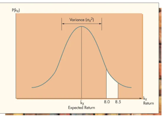
Like any random variable, the return on a stock investment has an associated probability distribution. Figure 8.3 is a graphic depiction of a probability distri-bution for the return on a stock we’ll call X. The return on X is called kX. The values the return can take appear along the horizontal axis, and the probabilities of those values appear on the vertical axis. The shape of the distribution depicts the likelihood of all possible actual values of kX according to areas under the curve.
The total area under the curve is 1.0, and the proportionate area under any sec-tion represents the probability that an actual return will fall along the horizontal axis in that area. For example, the shaded area in the diagram represents the probability that in any particular year the actual return on an investment in stock X will turn out to be between 8.0% and 8.5%. If that area is .1 or 10% of the total area under the curve, the probability of the actual return being between 8.0% and 8.5% in any year would be 10%. P(H) H 4' 10" 5' 8" 6' 6"
Figure 8.2
Probability Distribution for a Continuous Random Variable In financial theory, the return on a stock investment is considered a random variable.The mean or expected value (the most likely outcome) is usually found under the highest point of the curve. It’s indicated as kXin the diagram.
The mean is the statistical representation of the average investor’s expected re-turn that we talked about earlier. This is an important point. Portfolio theory as-sumes that all of the knowledge the investment community has about the future per-formance of a stock is reflected in the probability distribution of returns perceived by the investors. In particular, the mean of that perceived distribution is the expected return investors plan on receiving when they buy.
The variance and standard deviation of the distribution show how likely it is that an actual return will be some distance away from the expected value. A distribution with a large variance is more likely to produce actual outcomes that are substantially away from the expected value than one with a small variance.
Figure 8.3 shows the variance conceptually as the width of the distribution. We’ll use X2to indicate that we’re talking about the distribution of returns for stock X. Similarly, X will be the standard deviation for stock X. A large variance implies a wide distribution with gently sloping sides and a low peak. A narrow distribution with steeply sloping sides and a high peak has a small variance and standard devia-tion. Figure 8.4 shows distributions with large and small variances.
Notice that the large variance distribution has more area under the curve far-ther away from the mean than the small variance distribution. This pattern means that more actual observations of the return are likely to be far away from the mean when the distribution’s variance is large. Stated another way, returns will tend to be more different, or more variable, from year to year when the variance is large. When the variance is small, actual returns in successive years are more likely to cluster closely around the mean or expected value.
Figure 8.3
The Probability Distribution of the Return on an Investment in Stock XThe mean of the distribution of re-turns is the stock’s expected return. P(kX) kX Return Expected Return kX 8.0 8.5 Variance (σX2)
Risk Redefined as Variability
The meaning of risk in portfolio theory differs from the definition we gave earlier. Before we said that risk is the probability that return will be less than expected. In portfolio theory, risk is variability. That is, a stock whose return is likely to be sig-nificantly different from one year to the next is risky, while one whose returns are likely to cluster tightly is less risky. Stated another way, a risky stock has a high prob-ability of producing a return that’s substantially away from the mean of the distri-bution of returns, while a low-risk stock is unlikely to produce a return that differs from the expected return by very much.
But this is exactly the idea of variance and standard deviation that we’ve been talking about, so in portfolio theory, a stock investment’s risk is defined as the stan-dard deviation of the probability distribution of its return. A large stanstan-dard devia-tion implies high risk and a small one means low risk. In practical terms, high risk implies variabilityin return, meaning that returns in successive years are likely to be considerably different from one another.
Figure 8.4 can be interpreted as showing a risky stock and a low-risk stock with the same expected return. The difference is in the variances, which can be visually observed as the widths of the distributions.
This definition is somewhat inconsistent with the earlier version in which we said risk was the probability that return would be less thanwhat was expected. One would think that a more appropriate definition in statistical terms would equate risk with only the left side of the probability distribution, because in that area return is less than expected. Defining risk as the entire standard deviation includes the probabil-ity that the return turns out to be more than expected, and we’re certainly not con-cerned if that happens.
Indeed, a left-side-only definition would make more intuitive sense. However, it would be very difficult to work with mathematically. Theorists solved the problem
Figure 8.4
Probability Distributions with Large and Small Variances P(kX) kX Expected Return Small Variance (Low Risk) Large Variance (High Risk) kX Return In financial theory riskis defined as variabilityin return.
by noticing that return distributions are usually relatively symmetrical. This means that a large left side always implies a large right side as well. Why not therefore de-fine risk for mathematical convenience as total variability, understanding that we’re really only concerned with the probability of lower than expected returns (those on the left)? Indeed, this is what was done. The resulting technical definition of risk is a little strange in that it includes good news as well as bad news, but that doesn’t bother us if we keep the reason in mind.
So we actually have two definitions of risk that are both correct. In practical terms, risk is the probability that return will be less than expected. In financial theory, risk is the variability of the probability distribution of returns.
Terminology isn’t entirely consistent. When talking conceptually about risk, people are likely to use the terms “variance” or “variability.” But when a precise value is needed to represent risk in a mathematical equation, it’s more common to use , the standard deviation.
Notice also that defining risk as the probability that return will be less than ex-pected doesn’t tell us much. For more or less symmetrical distributions of returns, that probability will always be about 50%. But for some investments the return is never below the expected value by very much, while for others it can be below by a lot. The variance definition gets right at this distinction. If the distribution has a large variance, the return can be below the expected value by a substantial amount, and an investor can be hurt badly.
An Alternate View
There’s another way to visualize risk that many students find helpful. Imagine plot-ting the historical values of return on a particular stock over time. When we do that, we get an up-and-down graph like one of those shown in Figure 8.5. Over time the stock’s return is seen to oscillate around its average value, kX. The more the stock’s
Time Return kX A - High Risk B - Low Risk kX
Figure 8.5
Investment Risk Viewed as Variability of Return over Timereturn moves up and down over time, the more risky we say it is as an investment. That is, the greater the amplitude of the swings, the riskier the stock. This view is simply a graphic result of the variance of the distribution. In the diagram, stock A is relatively high risk and stock B is relatively low risk. We will use this representa-tion again shortly.
Risk Aversion
Now we’re in a position to define risk aversion more precisely. The axiom simply states that people prefer investments with less risk to those with more risk if the ex-pected returns are equal. Figure 8.6a illustrates the idea with probability distribu-tions. The narrower distribution has less risk and will be preferred to the wider, riskier distribution.
It’s important to understand that this preference is assumed to hold universally only in cases where the expected returns are exactly equal. When the choice is as illustrated in Figure 8.6b, the principle of risk aversion tells us nothing. There, in-vestment A is preferred on the basis of risk, while inin-vestment B is preferred on the basis of expected return. Which will be chosen depends on the individual investor’s tolerance for risk.
Risk aversion means investors prefer lower risk when expected returns are equal.
Figure 8.6
Risk Aversion
kA
k kB
Preferred Neither Preferred
with Certainty k k P(k) P(k) (a) (b)
Example 8.1
Evaluating Stand-Alone RiskThe notions of risk we’ve just developed are associated with owning shares of a single stock by itself. That can be characterized as stand-alone risk, because the stock’s variability stands alone independent of anything happening in the owner’s portfolio.
Harold MacGregor is considering buying stocks for the first time and is looking for a single company in which he’ll make a substantial investment. He has narrowed his search to two firms, Evanston Water Inc. and Astro Tech Corp. Evanston is a pub-lic utility supplying water to the county, and Astro is a relatively new high-tech com-pany in the computer field.
Public utilities are classic examples of low-risk stocks because they’re regulated monopolies. That means the government gives them the exclusive right to sell their products in an area but also controls pricing so they can’t take advantage of the public by charging excessively. The utility commissionusually sets prices aimed at achieving a reasonable return for the company’s stockholders.
On the other hand, young high-tech firms are classic examples of high-risk com-panies. That’s because new technical ideas can be enormously profitable, complete failures, or anything in between.
Harold has studied the history and prospects of both firms and their industries, and with the help of his broker has made a discrete estimate of the probability dis-tribution of returns for each stock as follows.
Evanston Water Astro Tech
kE P (kE) kA P (kA) 6% .05 100% .15 8 .15 0 .20 10 .60 15 .30 12 .15 30 .20 14 .05 130 .15
Evaluate Harold’s options in terms of statistical concepts of risk and return.
SOLUTION: First calculate the expected return for each stock. That’s the mean of each distribution.
Evanston Water Astro Tech
kE P (kE) kE*P (kE) kA P (kA) kA*P (kA) 6% .05 0.3% 100% .15 15.0% 8 .15 1.2 0 .20 0.0 10 .60 6.0 15 .30 4.5 12 .15 1.8 30 .20 6.0 14 .05 ____0.7 130 .15 19.5____ k E10.0% kA15.0%
Next calculate the variance and standard deviation of the return on each stock.
Evanston Water kE kEkE (kEkE)2 P (kE) (kEkE)2*P (kE) 6% 4% 16 .05 0.8 8 2 4 .15 0.6 10 0 0 .60 0.0 12 2 4 .15 0.6 14 4 16 .05 0.8___ Variance E22.8 Standard Deviation: E1.7%
Astro Tech kA kAkA (kAkA)2 P (kA) (kAkA)2*P (kA) 100% 115% 13,225 .15 1,984 0 15 225 .20 45 15 0 0 .30 0 30 15 225 .20 45 130 115 13,225 .15 1,984_____ Variance: A24,058 Standard Deviation: A63.7%
Finally, calculate the coefficient of variation for each stock’s return.
CVE .17 CVA 4.25
Discussion:If Harold considers only the expected returns on his investment options, he’ll certainly choose Astro. It’s most likely return is half again as high as Evanston’s. But a glance at the distributions reveals that’s not the whole story. With Evanston, Harold’s investment is relatively safe, because the worst he’s likely to do is a return of 6% rather than the expected 10%.
Investing in Astro is a completely different story. While Harold’s most likely return there is 15%, a substantial chance (15%) exists that he’ll lose everything. There’s also a 20% chance he’ll earn a zero return. Possibilities like these give people concerns about investing in this kind of stock.
It’s also important to appreciate the high side of the two distributions. With Evanston, Harold isn’t likely to do much better than the expected return, because the highest yield available is only 14%. The utility commission’s pricing regulations guar-antee that. But with Astro there’s a chance of more than doubling invested money in a relatively short time. That’s reflected in the 15% chance of a 130% return. That tends to offset the depressing loss possibilities in the minds of some investors.
It should be clear that on a stand-alone basis, Astro is a relatively risky stock, while Evanston is relatively safe. Astro’s risk and Evanston’s lack of it come from the vari-ationin the distributions of their returns, which we just observed by examining the distributions in detail. But the idea is also available in summarized form from the standard deviations and coefficients of variation.
First notice that Astro’s standard deviation is 63.7%. That means a “typical” re-turn has a good chance of being about 64% above or below the expected rere-turn of
15%. That’s an enormous range for return, from 49% to 79%. On the other hand,
Evanston’s standard deviation is only 1.7%, meaning a typical return will probably be less than two percentage points off the expected return.
It’s tempting to compare the two companies by saying Astro’s risk is (63.7/1.7) 37 times that of Evanston. But that’s not quite fair because Astro has a higher expected return. It makes more sense to compare the coefficients of variation, which state the standard deviations in units of their respective means. Evanston’s CV is .17 while Astro’s is 4.25, so it’s more reasonable to say that Astro is (4.25/.17) 25 times as risky as Evanston.
A picture is even more telling. Continuous approximations of the two distributions are plotted as follows.
63.7% 15% A k A 1.7 10.0 E k E
Decomposing Risk—Systematic (Market) and
Unsystematic (Business-Specific) Risk
A fundamental truth of the investment world is that the returns offered on various securities tend to move up and down together. They don’t move exactly together, or even proportionately, but for the most part, stocks tend to go up and down at the same times.
Events and Conditions Causing Movement in Returns
Returns on stock investments move up and down in response to various events and conditions that affect the environment. Some things influence all stocks, while oth-ers affect only specific companies. News of politics, inflation, interest rates, war, and economic events tend to move most stocks in the same direction at the same time. A labor dispute in a particular industry, on the other hand, tends to affect only the stocks of firms in that industry.
Although certain events affect the returns of all stocks, some returns tend to re-spond more than others to particular things. Suppose news of an impending reces-sion hits the market. The return on most stocks can be expected to decline, but not by the same amount. The return on a public utility like a water company isn’t likely to change much. That’s because people’s demand for water doesn’t change much in hard times, and the utility is a regulated monopoly whose profitability is more or less guaranteed by the government. On the other hand, the return on the stock of
So, after having said all that, which stock should Harold choose?
Although our analysis has laid out the solution clearly, no one but Harold can answer that question. That’s because his choice depends on his degree of risk aver-sion. Evanston is the better choice with respect to risk, but Astro is better with re-spect to expected return. Which dominates is a personal choice that only the investor can make.
The returnson securities tend to moveup and down together. 60% 30% 0 –100% 15% 30% 130% Evanston Astro 15% 10%
a luxury goods manufacturer may drop sharply, because recession signals a drying up of demand for the company’s product.
In short, there’s a general but disproportionate movement together upon which is superimposed a fair amount of individual movement.
Movement in Return as Risk
Remember that one way to look at a stock’s risk is to consider the up-and-down movement of its return over time as equivalent to that risk (Figure 8.5). Think of that total movement as the total risk inherent in the stock.
Separating Movement/Risk into Two Parts
It’s conceptually possible to separate the total up-and-down movement of a stock’s return into two parts. The first part is the movement that occurs along with that of all other stocks in response to events affecting them all. That movement is known as systematic risk. It systematically affects everyone.
The second part is whatever movement is left over after the first part has been removed. This movement is a result of events that are specific to particular compa-nies and industries. Strikes, good or bad weather, good or bad management, and demand conditions are examples of things that affect particular firms. This remain-ing movement is called unsystematic risk. It affects specific companies.
Systematic and unsystematic risk can also be called market risk and business-specific risk, respectively.
Portfolios
Most equity investors hold stock in a number of companies rather than putting all of their funds in one firm’s securities. We refer to an investor’s total stock holding as his or her portfolio.
Risk and Return for a Portfolio
Each stock in a portfolio has its own expected return and its own risk. These are the mean and standard deviation of the probability distribution of the stock’s return. As might be expected, the total portfolio also has its own risk and return.
The return (actual or expected) on a portfolio is simply the average of the re-turns of the stocks in it, where the average is weighted by the proportionate dol-lars invested in each stock. For example, suppose we have the following three-stock portfolio.
Stock $ Invested Return
A $ 6,000 5%
B 9,000 9
C ________15,000 11 $30,000
The return on the portfolio, expected or actual, is kpwAkAwBkBwCkC,
where kp is the portfolio’s return and the w’s are the fractions of its total value in-vested in each asset. The weighted average calculation is as follows.
A stock’s risk can be separated into systematic or marketrisk and unsystematic or business-specific risk.
Portfolios have their ownrisks and returns.
kp (5%) (9%) (11%) (.2)(.05)(.3)(.09)(.5)(.11)
9.2%
The risk of a portfolio is the variance or standard deviation of the probability distribution of the portfolio’s return. That depends on the variances (risks) of the returns on the stocks in the portfolio, but not in a simple way. We’ll understand more about this relationship of portfolio risk to stock risk as we move on.
The Goal of the Investor/Portfolio Owner
As we said earlier, the goal of investors is to capture the high average returns of equities while avoiding as much of their risk as possible. That’s generally done by constructing diversified portfolios to minimize portfolio risk for a given return.
Investment theory is based on the premise that portfolio owners care only about the financial performance of their whole portfolios and not about the stand-alone characteristics of the individual stocks in the portfolios.
In other words, an investor evaluates the risk and return characteristics of a new stock only in terms of how that stock will affect the performance of his or her port-folio and not on the stand-alone merits of the stock. How a stock’s characteristics can be different in and out of a portfolio will become clear shortly.
Diversification—How Portfolio Risk Is Affected When
Stocks Are Added
Our basic goal in investing, to capture a high portfolio return while avoiding as much risk as possible, is accomplished through diversification. Diversification means adding different, or diverse, stocks to a portfolio. It’s the investor’s most basic tool for managing risk. Properly employed, diversification can reduce but not eliminate risk (variation in return) in a portfolio. To achieve the goal, however, we have to be careful about how we go about diversifying. We’ll need to address unsystematic (business-specific) risk and systematic (market) risk separately.
Business-Specific Risk and Diversification
If we diversify by forming a portfolio of the stocks of a fairly large number of dif-ferent companies, we can imagine business-specific risk as a series of essentially ran-dom events that push the returns on individual stocks up or down. The stimuli that affect individual companies are separate events that occur across the country. Some are good and some are bad.
Because events causing business-specific risk are random from the investor’s point of view, their effects simply cancel when added together over a substantial number of stocks. Therefore, we say that business-specific risk can be “diversified away” in a portfolio of any size. In other words, the good events offset the bad ones, and if there are enough events the net result tends to be about zero.
However, a word of caution is in order. For this idea to work, the stocks in the portfolio have to be from companies in fundamentally different industries. For ex-ample, if all the companies in a portfolio were agricultural, the effect of a drought wouldn’t be random. It would hit all of the stocks. Therefore, the business-specific risk wouldn’t be diversified away.
$15K $30K $9K $30K $6K $30K
Investors are con-cerned with how stocks impact port-folio performance and not with their stand-alone characteristics.
Business-specific riskis essentially random and can be diversified away.
This is an easy but powerful concept. For investors who hold numerous stocks, business-specific risk simply doesn’t exist at the aggregate level because it’s “washed out” statistically. Individual stocks still have it, but portfolios do not, and the port-folio is all the investor cares about.
Systematic (Market) Risk and Diversification
Reducing market risk in a portfolio calls for more complicated thinking than does handling business-specific risk. It should be intuitively clear that if the returns of all stocks move up and down more or less together, we’re unlikely to be able to elim-inate all of the movement in a portfolio’s return by adding more stocks. In fact, sys-tematic or market risk in a portfolio can be reduced but never entirely eliminated through diversification. However, even the reduction of market risk requires careful attention to the risk characteristics of the stocks added to the portfolio.
The Portfolio
To appreciate the issue, imagine we have a portfolio of stocks that has an expected return kp. In what follows, we’ll assume for simplicity that all the stocks have the same expected return. It’s all right to make this unrealistic assumption for illustra-tive purposes, because the points we’re getting at involve the interplay of risk among stocks and not of returns.
Our portfolio will have its own risk or variation in return, which is determined by the stocks in it. We’ll assume the portfolio has been put together to mirror ex-actly the makeup of the overall stock market. That is, if the prices of the stocks in the overall market are such that General Motors makes up 2% of the market’s value, we’ll spend 2% of our money on General Motors stock, and so on through all the stocks listed on the market. If the portfolio is constituted in this way, its return will move up and down just as the market’s return does. In other words, the portfolio’s risk will just equal the market’s risk. The behavior of the portfolio’s return over time is illustrated in Figure 8.7 by the heavy line labeled P.
Return, k kp kp Time B P C A
Figure 8.7
Risk in and out of a Portfolio
The Impact on Portfolio Risk of Adding New Stocks
We now want to consider the impact on the portfolio’s risk of adding a little of eitherof two new stocks to it. We’ll call these stocks A and B. The special behavior of the return on each is shown in Figure 8.7. Notice that we’re not talking about adding both stocks A and B at the same time. Rather the idea is to assess the im-pact on the risk of the resulting portfolio of adding a little of A ora little of B to the original portfolio.
First consider stock A. What happens to the risk of the portfolio if we add a few shares of A? Notice that A’s return achieves its highs and lows at exactly the same times as does the portfolio’s, and that its peaks and troughs are higher and lower, respectively, than the portfolio’s. It should be clear that the inclusion of a little A will tend to heighten the portfolio’s peak returns and depress its lowest returns. In other words, it will make the swings in the portfolio’s return larger. That means it will add risk to the portfolio.
In statistical terms, A’s return is said to be perfectly positively correlated with the portfolio’s return. That means the two returns move up and down at exactly the same times. Such stocks will generally add risk to a diversified portfolio.
Now consider the pattern of returns on stock B over time. Its peaks occur with the portfolio’s valleys, and its valleys coincide with the portfolio’s peaks. The return on stock B is always moving up or down in a direction opposite the movement of the return on the portfolio.
What will happen to the pattern of returns of the portfolio if we add a few shares of B? Clearly, the peaks will be lower and the valleys will be higher—that is, the swings won’t be as wide. According to our definitions, that means the risk will be lowered by adding some B. In statistical terms, B’s return is said to be perfectly neg-atively correlated with the portfolio’s return. Such stocks will always lower the port-folio’s risk.
In short, A adds risk to a portfolio while B reduces the portfolio’s risk.
The Risk of the New Additions by Themselves and in Portfolios
Now consider the relative riskiness of stocks A and B without reference to a port-folio. That is, how risky is each one standing alone? Figure 8.7 shows that A’s and B’s returns have about the same level of variation. That is, their peaks and troughs are about the same height. Therefore, their stand-alone risks as individual stocks are about the same.
However, in a portfolio sense, A is risky and B is safe in that A adds and B subtracts risk. This is a central and critically important concept. Although A and B are equally risky on a stand-alone basis, they have completely opposite risk impacts on a portfolio.
The portfolio definition of a stock’s risk is related to the timing of the variabil-ity of the stock’s return rather than to the magnitude of the variation. It has to do with the way the new stock’s return changes when the portfolio’s return changes. Or, if the portfolio is constituted like the market as we’ve assumed, it has to do with the way the stock’s return changes with the return on the market.
However, the degree to which a stock’s return moves with the market is what we’ve called market risk. Hence, we can say that a stock’s risk in a portfolio sense is its market risk.
Stocks with equal stand-alone risk can have opposite risk impacts on a portfoliobecause of the timing of the variations in their returns.
Choosing Stocks to Diversify for Market Risk
How do we diversify to reduce market risk in a portfolio? Figure 8.7 might imply that it’s easy: Just add stocks like B until the movement of the portfolio is virtually dampened out. Unfortunately, stocks like B that move countercyclically with the mar-ket are few and far between.
The classic example of such a stock involves shares in a gold mine. When returns on most stocks are down, people flee from paper investments and put money in tan-gible assets, notably gold. That drives the price of gold up. A higher price for gold means a gold mine becomes more profitable, which elevates the return on its stock. Hence, when the return on most stocks is down, the return on gold mine stocks tends to be up. The reverse happens when stock returns are generally high.
Although people do diversify with gold mine stocks to stabilize portfolios, there aren’t enough of them to do the job thoroughly. There simply aren’t many stocks around that are negatively correlated with the market.
However, a great number of stocks are available whose returns behave in a man-ner somewhere between those of A and B in the diagram. In terms of the behavior of return, that kind of stock can be thought of as a combination of A and B. Such a stock is illustrated by line C in Figure 8.7. Stocks like C are said to be not per-fectly positively correlated with the portfolio.
Adding some C to the portfolio will generally reduce its risk somewhat. If we think of C as a hybrid or cross between A and B, its addition is a way to get a little B into the portfolio indirectly. An intuitive way to put it is to say that C contains a little of the “personality” of B.
In summary, market risk generally can be reduced but not eliminated by diversi-fying with stocks like C that are not perfectly positively correlated with the portfolio. The Importance of Market Risk
Let’s return to stocks A and B in Figure 8.7 for a moment. The illustration is con-structed to point out two different concepts of risk. Considered individually, the stocks are equally risky, yet in a portfolio one is risky and the other is not. Which interpretation is appropriate and when?
The relative risk attributes of the two stocks are entirely changed if we assume in-vestors focus on portfolios rather than on individual stocks. Modern portfolio theory is based on that assumption. What matters is how stocks affect portfolios rather than how they behave when considered alone. And how they affect portfolios depends only on market risk. This is a fundamental result of portfolio theory. According to the theory, what matters in the investment world is market risk alone. It is also a dangerous result. Business-specific risk is truly diversified away only in the context of large portfolios. For the small investor with a limited portfolio, that effect simply doesn’t occur. An individual business reversal can devastate an investment program if the stock repre-sents a significant portion of a small portfolio. Hence, while the thinking behind portfolio theory may be appropriate for running a mutual fund, it should not be ap-plied blindly to managing one’s personal assets.
Measuring Market Risk—The Concept of Beta
Because market risk is of such central importance to investing, it’s appropriate to look for a way to measure it for individual stocks.
Market risk in a portfolio can be reduced but not eliminated by diver-sifying with stocks that are not per-fectly positively correlatedwith the portfolio.
Caution:The con-cepts of risk associ-ated with portfolio theory may not be appropriate for indi-vidual investors.
A statistic known as a stock’s betacoefficient has been developed that is com-monly considered to be the measure of a stock’s market risk. Essentially, beta cap-tures the variation in a stock’s return which accompaniesvariation in the return on the market.
Developing Beta
A stock’s beta coefficient is developed by plotting the historical relationship between the return on the stock and the return on the market.2Figure 8.8 shows such a plot. Each point represents a past time period for which we plot the stock’s return, kX, on the vertical axis and the market’s return, kM, on the horizontal axis. Doing this for a number of past periods results in a “scatter diagram” of historical observations. A re-gression line fitted to these data points is known as the characteristic linefor the stock.
2. The return on the market is estimated by calculating the return on a market index such as the Standard & Poor’s 500.
A stock’s beta measures its market risk. kX kM ∆ kM ∆ kX Values of (kM, kX) Characteristic Line ∆ kM ∆ kX Slope = = bX = Beta
Figure 8.8
The Determination of Beta A stock’s character-istic linereflects the average rela-tionship between its return and the mar-ket’s. Beta is the slope of the charac-teristic line.The characteristic line represents the average relationship between the stock’s return and the market’s return. Its slope is particularly rich in information. The slope tells us on the average how much of a change in kX has come about with a given change in kM. This is exactly what we’re looking for in terms of measuring market risk. The slope is an indication of how much variation in the return on the stock goes along with variation in the return on the market.
To see this, notice that as we move along the characteristic line, a change in kM, kM, comes with a change in kX, kX. The relationship between these changes is re-flected in the slope of the line.
(8.3)
slope bXbeta kX kM rise runIS IT INVESTING OR GAMBLING?
Investing is putting money at risk in the hope of earning more money—a return. But isn’t that also a definition of gambling? Certainly it is, so what’s the difference between investing and gambling, and why do we have such different moral and ethical atti-tudes about them?
Investing has economic value to the society that gambling doesn’t. But, aside from that, from an individual’s perspective it’s fair to ask about the distinction between playing the stock market and taking a trip to Las Vegas.
Viewing both processes in terms of the probability distributions of their returns pro-vides some insight. Investing tends to be characterized by probability distributions with positive expected values (means) and relatively small probabilities of very large gains or losses. Gambling on the other hand generally has a zero or negative expected value and offers a good chance of losing everything placed at risk. The attraction of gambling is that there’s also a visible chance of winning many times the amount risked along with its entertainment value. Think of playing roulette in a Las Vegas casino. It’s no se-cret that the odds are stacked slightly in favor of the house, and that many visitors leave town with empty pockets. But there are also a few well-publicized examples of people who hit the jackpot. Graphically, the distributions might look something like this.
INSIGHTS
PRACTICAL FINANCE
This view leads to another logical question. Are there activities that people normally call investing that are more like gambling? The answer is a resounding yes. Buying the stock of a high-risk new venture might be an example. There are also some financial markets that are risky to the point of bordering on gambling (e.g., commodities and futures markets, which are beyond the scope of this book).
In fact, the whole idea of portfolio theory is to move the investor’s exposure toward the investment profile we’ve just described and away from the gambling profile.
The important thing to take away from this discussion is that something isn’t “in-vesting” just because it happens through the financial industry. Brokers like to char-acterize all their offerings as investing because it has a nobler image. But, in fact, some financial “investments” are really more like gambles.
0% 100% +
–100%
Investing Gambling
Market risk is defined as the degree to which the return on the stock moves with the return on the market. That idea is summarized perfectly by the slope of the char-acteristic line. The slope can therefore be definedas the measure of market risk for the stock. This measure is called the beta coefficient, or simply beta, for the stock. Projecting Returns with Beta
Knowing a stock’s beta enables us to estimate changes in its return given changes in the market’s return.
Example 8.2
Conroy Corp. has a beta of 1.8 and is currently earning its owners a return of 14%. The stock market in general is reacting negatively to a new crisis in the Middle East that threatens world oil supplies. Experts estimate that the return on an average stock will drop from 12% to 8% because of investor concerns over the economic impact of a potential oil shortage as well as the threat of a limited war. Estimate the change in the return on Conroy shares and its new return.SOLUTION: Beta represents the past average change in Conroy’s return relative to changes in the market’s return.
bConroy
Substituting,
1.8
kConroy7.2%
The new return can be estimated as
kConroy14%7.2%6.8%. kConroy 4% kConroy kM Understanding Beta
It’s important to understand that beta represents an average relationship based on past history. To appreciate this, consider the movement from one data point to the next in Figure 8.8.
The change between any two successive values of kXrepresents movement caused by the combination of market risk forces and business-specific risk forces. In other words, such a change is part of the stock’s total risk. By regressing kX versus kM, we’re making the assumption that movement along the line representing an average relationship between the variables reflects only market-related changes. In this view, movement from one data point to the next has two components, movement to and from the line and movement along the line. Movement to and from the line repre-sents business-specific risk, while movement along the line reprerepre-sents market risk. Forecasting with beta, as in the last example, uses only the average relationship between the returns, which is assumed to be market related. It says nothing about business-specific risk factors.
Beta over Time
Any firm’s beta is derived from observation of the behavior of its return in the past relative to the return on the market. Use of the statistic implicitly assumes that the relationship between the two returns is going to remain constant over time. In other words, using beta assumes the stock’s return will behave in the same way in the future that it did in the past relative to the market’s return. This assumption is usually reasonable, but at times it may not be.
Example 8.3
Suppose Conroy Corp. in Example 8.2 is a defense contractor that makes sophisti-cated antimissile systems. Would the estimate of return done in that example be valid? What if Conroy were in the orange juice business?SOLUTION: It’s unlikely that the estimate would be much good if Conroy were a defense contractor. The threat of a limited war could be expected to have a positive impact on the company because of its defense-related line of business. In other words, such a threat is likely to have a major business-specific risk impact on the firm’s return that would act in a direction opposite the market-related decline.
If Conroy made orange juice, we wouldn’t expect a business-specific risk change due to the Middle East crisis, so the market-related estimate would be more realistic.
Betas are devel-oped from historical dataand may not be accurateif a funda-mental changein the business envi-ronment occurs.
Example 8.4
Let’s consider the Conroy Corp. of the last two examples once more. Think of the early 1990s when the Cold War was ending and military budgets were being reduced dramatically. Would a projection using beta have been valid at that time?SOLUTION: In this situation the value of Conroy’s beta is uncertain. The data from which the firm’s characteristic line was developed would have been from earlier periods during the Cold War when military spending and lucrative defense contracts were considered a way of life that was likely to continue forever. The early 1990s were characterized by a climate of reduced defense budgets which made high-technology defense production look a lot more risky. Therefore, the future beta is likely to have been different from the past value at that time.
Volatility
Beta measures volatility in relation to market changes. In other words, it tells us whether the stock’s return moves around more or less than the return of an average stock.
A beta of 1.0 means the stock’s return moves on average just as much as the mar-ket’s return. Beta 1.0 implies the stock moves more than the market. Beta1.0 means the stock tends to move with the market but less. Beta 0 means the stock tends to move against the market, that is, in the opposite direction. Such stocks are rare. Stock B of Figure 8.7 is a negative beta stock. Gold mines are the primary real-world example of such stocks.
The idea of beta immediately suggests an investment strategy. When the market is moving up, hold high-beta stocks because they move up more. When the market is moving down, switch to low-beta stocks because they move down less!
Small investors should remember that beta doesn’t measure total risk.