Graph partitioning for the reduction of data transfer in task-based programming models

(1)

Master of Science in

Advanced Mathematics and

Mathematical Engineering

M

A

ST

ER

’S

D

EG

R

EE

TH

ES

IS

Title: Graph partitioning for the reduction of data transfer in task-based programming models

Author: Isaac Sánchez Barrera

Advisors: Marc Casas Guix (BSC-CNS)

Miquel Moretó Planas (UPC / BSC-CNS) Departments: Computer Architecture (UPC)

Computer Sciences (BSC-CNS) Academic year: 2015-2016

(2)

(3)

Graph partitioning for the reduction of data

transfer in task-based programming models

Master’s degree thesis

Author:

Isaac Sánchez Barrera

Opting for the Master of Science in Advanced Mathematics and Mathematical Engineering

Advisors:

Marc Casas Guix

Department of Computer Sciences Barcelona Supercomputing Center

Miquel Moretó Planas

Department of Computer Architecture Universitat Politècnica de Catalunya Department of Computer Sciences Barcelona Supercomputing Center

Facultat de Matemàtiques i Estadística

Universitat Politècnica de Catalunya

RoMoL Project

(4)

(5)

A mi hermana, Marta. Porque sí.

(6)

(7)

Abstract

Current high performance computing architectures are composed of large shared memory NUMA nodes, among other components. Such nodes are becoming increasingly complex as they have several NUMA domains with different access latencies depending on the core where the access is issued.

In this work, we propose techniques to efficiently mitigate the negative impact of NUMA effects on parallel applications performance. We leverage runtime system metadata ex-pressed in terms of a task dependency graph, where nodes are sequential pieces of code and edges are control or data dependencies between them, to efficiently reduce data transfers using graph partitioning techniques. With our proposals, we are able to im-prove the execution time of OpenMP parallel codes a factor of 2.02× on average when run on architectures with strong NUMA effects.

Resum

Les arquitectures per a computació d’altes prestacions actuals estan formades per grans nodes NUMA (amb accessos a memòria no uniformes) de memòria compartida, entre d’al-tres components. Aquests nodes estan incrementant la seva complexitat donat l’increment en la quantitat de dominis NUMA amb latències diferents segons la unitat de procés des d’on s’ha sol·licitat l’accés a les dades.

En aquest treball proposem tècniques per tal de reduir l’impacte negatiu dels efectes NUMA en el rendiment d’aplicacions paral·leles. Fem servir les dades del sistema expressa-des com a un graf de dependències, on els vèrtexs són peces de codi seqüencial i les arestes són dependències de dades o control entre elles, per tal de reduir les dades transferides mitjançant tècniques de particionat de grafs. Amb aquestes propostes, som capaços de millorar el temps d’execució de codis paral·lels OpenMP amb un factor 2.02×de mitjana en arquitectures que tenen grans efectes NUMA.

MSC2010: 68M07 (primary), 68M20, 68R10.

(8)

(9)

Acknowledgements

One year and a half ago, nearly at the end of January, I presented my Bachelor’s thesis at Facultat d’Informàtica de Barcelona, and so did my good friend Guillermo. If I recall correctly, that same day (or maybe it was a week later? Don’t think so) Francesc asked us what we were going to do after having finished our undergradu-ate studies. Guillermo had just found a job, but I was wondering myself what I would do... I knew I wanted to continue studying, and probably focus my career in doing research, but I didn’t have any clue. Luckily enough, Francesc asked us because he had been doing an internship at the Riding on Moore’s Law project (RoMoL) at BSC during the summer and knew they were looking for some student to join the team.

Fast-forward a couple of weeks and I had meeting scheduled with Marc and Miquel. A week before meeting them, I had another meeting with Maria Serna, the advisor for my Bachelor’s thesis. She asked about my future, and I told her about my meeting at BSC. We also talked about the studies, and she recommended me to do the MAMME, and I am deeply thankful for that (I was a bit scared of MAMME at first, even though I had also studied Mathematics, and didn’t think about doing it until she told me to).

In my meeting with Marc and Miquel a week later I told them about doing the MAMME and they thought it was a good idea. They had both studied a Bachelor’s degree in Mathematics at FME when they were 5-year-long, anyway, so they knew what it was about. They presented different projects and one of them was the work Francesc had started about graph partitioning (he didn’t continue because he was more into number theory, but he did a good start), and here I am now.

I’m going to switch languages for a bit, I will come back to English a bit later. Dit això, t’he de donar les gràcies, Francesc, per haver-me posat en contacte amb en Miquel i en Marc, va ser la proposta adequada en el moment adequat, i espero que t’ho passis bé jugant amb la proporció àuria (ja saps). També us estic molt agraït a vosaltres, Marc i Miquel, per l’oferta i per tota l’ajuda que m’heu donat (i m’esteu donant) amb aquest projecte. Especialment perquè m’agrada prendre’m les coses amb calma. I perquè gràcies a això tinc programats els propers anys, cosa que no és fàcil.

No me puedo olvidar de ti, Alberto, que tanto nos hemos soportado los me-diodías, y más veces, también intentando que se mueva el puñetero dragón de colorines, que sobreviva hasta pasado julio, y haciendo muchas más cosas porque tenemos mucho tiempo libre. Y Alejandro, que también has estado muchos

(10)

me-haya visto poco, Guillermo y Alex, tampoco me olvido de vosotros, que siempre estais ahí como cuando fuimos a ver a Ander con Alberto y Francesc; y de quien tampoco me olvido es de Ander, que nos invitaste a tu casa y pasamos un muy buen fin de semana lleno de oportunidades. Seguro que pronto nos volvemos a ver. Y aunque Marta no nos acompañó, para variar, tampoco puedo olvidarme de nombrarla, que este año la he visto casi más que cuando estábamos haciendo el grado.

Casi acabamos, y no me olvido de mi familia. Este año ha estado lleno de nove-dades para los cuatro (y los seis, si contamos a los chuchos) y creo que en general es todo bueno. Especialmente para ti, Marta, que por fin has encontrado lo que te gusta. Y que siempre te alegras por mí.

Getting back to English, I will also say a big “thank you” to all of you at the RoMoL team, past and present. It’s great working with you and having you avail-able to answer any doubts. The things I’ve learnt with you, the good working environment..., everything has been great and will continue like so.

A punt he estat d’oblidar-me, però per sort me n’he recordat... Moltes gràcies al Cor de noies i en especial a l’Helena per comptar amb els antics nois de la Coral juvenil per fer aquests concerts tan especials. Ha estat un plaer passar els divendres a la tarda un altre cop a l’escola de música.

Last but not least, a few acknowledgements. This project has been partially supported by the RoMoL ERC Advanced Grant (GA 321253), the European HiPEAC Network of Excellence and the Spanish Ministry of Economy and Competitiveness under contract Computación de Altas Prestaciones VII (TIN‐201565316‐P).

(11)

1 Introduction

1.1 Problem background

Since the end of Dennard scaling and the subsequent stagnation of the CPU clock frequency, computing infrastructures can only increase their peak performance via augmenting their number of computing units. In the High Performance Comput-ing (HPC) context, this trend has brought an increase in the hardware components count as well as in the heterogeneity among them. As such, shared memory nodes, which are fundamental building blocks of HPC infrastructures, are experiencing an increase in the number of sockets they integrate. Besides the benefits in terms of a unified flat memory address space and large core counts, integrating many sockets into the same node exacerbates its Non-Uniform Memory Access (NUMA) effects, which can become a serious performance bottleneck if they are not prop-erly handled. For example, synchronisation operations or barriers can seriously slowdown the whole parallel execution if software components that access locally stored data remain idle while waiting for other software components accessing remote data to reach the barrier.

Figure 1.1:Example of a NUMA topology with two pairs of NUMA nodes, gener-ated using the lstopo tool from hwloc, the Portable Hardware Loca-tion package [6], [21].

To mitigate NUMA effects, techniques con-sisting in migrating threads, memory pages or both already exist [15], [16], [41]. These techniques aim to move either computa-tion or data to reduce memory access time. Even though they effectively mitigate NUMA effects, they do not exploit any kind of application-specific information to predict ac-cesses to remotely allocated data before a par-ticular software component starts displaying this behaviour. As such, already proposed OS-level thread or page migration techniques can only take action when the application is

already suffering from remote memory accesses, which ends up bringing subop-timal solutions in most of the cases. Oppositely, other approaches transfer the NUMA management responsibility to the programmer [30], [44], exploiting

(14)

in-formation at the application source code level to carry out NUMA-aware schedul-ing decisions. However, these approaches require significant code refactorschedul-ing and programmer effort to be effective.

1.2 Task-based parallelism and its opportunities in NUMA

systems

This section describes the main characteristics of task-based programming models together with their potential to mitigate NUMA effects on large shared memory systems.

1.2.1 Task-based programming models

The most common way to program shared memory nodes are thread-based pro-gramming models like OpenMP [32] or Pthreads [11]. The OpenMP standard has support for tasking and dependencies since version 4.0, which means that the ap-plication source code is split into several pieces called tasks, with their data or control dependencies explicitly indicated by means of #pragma compiler direct-ives. A directed acyclic graph where nodes represent tasks and edges express the dependence between them is maintained by the runtime system to orchestrate the parallel execution and is commonly referred as the application’s Task Dependency Graph (TDG).

Building the task dependency graph

In a task-based data-flow programming model like OpenMP 4.0, the programmer does not indicate the dependencies between tasks explicitly but by means of the pieces of data that are read from or written to. The runtime system is then the one in charge of building the task dependency graph with this information. This can create various kinds of dependence relations between the tasks. Consider taskA

should occur in time before taskBif they were executed sequentially; if they use data that is stored in the same place, we can have the following three options:

flow dependency Also know as read-after-write (RAW), when Breads from where

(15)

1.2 Task-based parallelism and its opportunities in NUMA systems

anti-dependency Also known as write-after-read (WAR), when B writes whereA

reads from.

output dependency Also know as write-after-write (WAW), whenBand Awrite to the same place but Bdoes not read from there.

In these cases it is important that B is executed after A, or at least that some kind of data consistency method is used, otherwise the result might not be correct. See that there is no read-after-read option: when two consecutive tasks want to just read from the same place (not write), there is no risk that one modifies the data needed by the other one

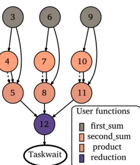
As an example, consider that we have three vectorsu,v,w ∈ ℝ3 and we want to calculatez= ⟨u+v,v+w⟩ ∈ ℝ. Algorithm 1.1 is a sample version coded in C, with the TDG in figure 1.2. It is not an efficient way to do it, but it will serve to show flow and anti-dependencies.

Algorithm 1.1:Small task-based program

double foo(double u[3], double v[3], double w[3]) {

double z = 0.0;

for (int i = 0; i < 3; ++i) {

#pragma omp task inout(u[i]) in(v[i]) label(first_sum) {

u[i] = u[i] + v[i];

}

#pragma omp task inout(v[i]) in(w[i]) label(second_sum) {

v[i] = v[i] + w[i];

}

#pragma omp task in(u[i], v[i]) out(w[i]) label(product) {

w[i] = u[i] + v[i]

} }

#pragma omp task in(w[0], w[1], w[2]) out(z) label(reduction) {

z = w[1] + w[2] + w[3]; }

#pragma omp taskwait

return z;

(16)

User functions 3 4 5 12 6 7 8 9 10 11 Taskwait first_sum second_sum product reduction

Figure 1.2:Task dependency graph for algorithm 1.1. Solid arcs show flow dependencies, dashed arcs show anti-dependencies. Numbers represent the execution order in the sequential case.

The algorithm stores the sumu+voverwritingu, andv+woverwritingw. Output dependencies might not seem useful at first. However, they are in the case of stencil algorithms that work by saving in every cell the average of the neighbouring cells, such as stationary heat diffusion algorithms.

1.2.2 Suitability for NUMA-aware scheduling

The runtime system is in charge of managing the parallel execution, releasing the programmer from the burden of explicitly expressing task synchronisation or scheduling at the application source code level. In this way, tasks are scheduled to cores once their data or control dependencies are satisfied. A key aspect of this data-flow execution model is the explicit knowledge the runtime system has in terms of the ranges of memory addresses that are going to be accessed by tasks before they actually start running, which enables improvements in terms of data prefetching [33] or cache coherence protocol optimizations [26]. In this context, our work is the first in showing the need for dynamic graph partitioning at the runtime system level to exploit data locality and mitigate NUMA effects on large shared memory systems without programmer intervention.

Task-based data-flow programming models are specially well suited for large shared memory systems with NUMA effects. The specification of the input and

(17)

1.2 Task-based parallelism and its opportunities in NUMA systems output dependencies for the tasks provide the runtime system with the information of what data is going to be accessed. Also, the runtime system has the knowledge of where the data resides within the NUMA regions of the node. In this case, it is possible to schedule a given task in a thread local to the NUMA region where its required data resides, thus avoiding the cost of increased latency and bandwidth waste which might otherwise be experienced by scheduling the task at a larger NUMA distance from its data. This NUMA-aware scheduling also provides a higher probability for a task to hit its data in the Last-Level Cache (LLC) of the processor if previous tasks using this data also ran in the same socket. As a consequence, memory accesses to inputs and outputs will always accessclose memories during the execution of tasks, exploiting the data locality of the application as a result.

1.2.3 Task scheduling in NUMA systems

The typical behaviour of a thread in a task-based runtime system consists in re-questing tasks to the scheduler, executing them and notifying about task com-pletions to enable the wake up and execution of dependent computations. Once a thread sends a request to the runtime system, a task is picked up based on a certain policy. A very simple one consists in selecting tasks based on a First-In First-Out (FIFO) regime without any other consideration. To improve data local-ity, a simple optimisation consists in scheduling the immediate successor: When a task has a dependent computation and it is the only remaining parent to finish, the thread executing that task selects the dependent computation to be run right after parent’s execution finishes. However, this optimisation does not consider the data location of previously finished parent tasks. As an alternative, some authors propose to enrich the Application Programming Interface (API) of the runtime sys-tem, so that the programmer can manage data placement and exploit data locality by specifying the socket where the task should be executed [17], [30]. These ap-proaches also implement a distance-aware work-stealing method that steals tasks from the closest NUMA regions, which allows reducing load imbalance. However, they are not automatic, increasing the programmability burden in parallel systems. Alternatively, in this work we propose to leverage the information contained in the TDG to automatically mitigate NUMA effects without any specific programmer intervention.

(18)

1.3 Graph partitioning

1.3.1 The graph partitioning problem

In this work we are going to show the usefulness of graph partitioning techniques to improve the performance of task-based applications in NUMA systems. A good general definition for the graph partitioning problem is that from a recent survey in graph partitioning and its applications by Buluç et al. [10]. This definition is the one given in problem 1.1.

Problem 1.1(Graph partitioning).Given a positive integerkand an undirected graph

G= (V,E)with positive edge weightsω:E⟶ ℝ+, find a partitionΠ = (V₁, … ,V_k)

of the set of vertices.

In general, we want partitions that are balanced, that is |V_i| ≤ (1+ε)⌈V/k⌉ for some ε ≥ 0, and such that some metric is minimal. If we define the mapping

φ:V ⟶ 1, … ,k that assigns every vertex to the partition where it belongs, or

φ(v) =iifv∈ V_i inΠ, we want to minimise the objective function

􏾝

uv∈E

φ(u)≠φ(v)

ω(uv).

This function is known as theedge-cut of the solution and corresponds to the total weight of the edges connecting pairs of vertices from two different parts inΠ.

Under these constraints, the problem is np-hard, but it has been studied for many years and there are known algorithms and heuristics for approximating it [10]. Some of the available libraries in the HPC scenario are Metis [24], [25], Scotch [36], [37] and the Zoltan framework [5]. In fact, these libraries have been developed mostly to reduce the data transfer in parallel systems, but for the case of message-passing applications (which can be seen asundirected graphs).

1.3.2 Graph partitioning algorithms

In this work we will use standard graph partitioning tools for undirected graphs to partition the TDG of applications, which are directed acyclic graphs. Here we give a brief summary of the algorithms used in the Scotch library by Pellegrini [36, 37]. Our main reference for this is Scotch User’s Guide [35].

(19)

1.3 Graph partitioning

Dual recursive bipartition

This is one of the most basic and used methods. It is a recursive divide-and-conquer algorithm that consists in doing a2-partition of the set of parts, and a2-partition of the set of vertices and map the last two to the pair of sets of parts. The mapping is done recursively until what is assigned is a set of tasks to a single part. The bipartitions are done using some heuristics that use the information from the edge weights to make good decisions.

Multilevel mapping

Rather than a partitioning/mapping algorithm, this is a scheme to do the partition in an easier way or with higher quality. It coarsens the input graph (makes it more rough, joining vertices), then applies the partitioning algorithm to the coarsened graph, projects back the partition to the original graph and refines it. This is quite well shown in figure 3 from the user manual [35].

Diffusion

It is a general method that, in the case of a bipartition, is easily understood with a metaphor. Two vertices are selected (using some heuristic) and one of two antagonistic liquids are poured into them (we can also think of the liquids as matter and anti-matter). In every vertex a bit of the liquid is lost, and the vertex gets to the part of the liquid that has arrived with more quantity. They annihilate each other (and hence the comparison with matter and anti-matter).

Fiduccia-Mattheyses

This algorithm is a local-search algorithm somewhat extended not to stall in a local minimum. Starting with a given partition, it tries to improve it by moving vertices from one partition to another.

1.3.3 Related work and existing results using graph partitioning

Graph partitioning has been used for long time to assign tasks to processors in parallel machines, as commented by Pellegrini [37]. This has been done mostly in two ways, one is dividing the data graph, where every vertex corresponds to a

(20)

block of data and the adjacencies come from the simultaneous use of the data in a task/process. The other one is a process graph, mostly related to message-passing programming models, where each vertex corresponds to one of the processes and the edges show the communications between them. Our work is the first to apply graph partitioning during execution time in a shared-memory system, while pre-vious approaches partition the graph statically (in advance, not in real time) or focus on distributed memory systems.

One of the most recent developments to guide task schedulers via graph parti-tioning techniques is SPAWN by Papinet al. [34]. This approach takes advantage of sophisticated properties of the graph that are extracted from the input data and the application source code. The process of building the graph is considerably complex as it requires a precise understanding of the targeted application source code and its input, needing the help of the programmer to define distances in the physical domain of the application, which is something our approach does not require since the graph is generated on runtime without the need for any specific programmer intervention.

SPAWN works by building a graph representing the physical domain of the prob-lem solved by the application and embed it on a geometric space. Initially, the processing elements of the target machine executing the parallel application are uniformly distributed on the region occupied by the problem domain (giving an electrical charge to each element), and the domain is partitioned using a Voro-noi tessellation. As the time advances, the electrical charges of the processing elements are modified according to their work load, inducing a new Voronoi tes-sellation and effectively fixing possible load imbalances.

There have been previous results in partitioning directed acyclic graphs us-ing standard partitioners. For example, Tanaka and Tatebe [40] used the multi-constraint capabilities of METIS to schedule workflows, which are more coarse-grained than usual shared-memory task dependency graphs. Using an approach with multiple load balance constraints, the vertices have anr-dimensional weight (for some constant r) and the target parts also have an r-dimensional capacity each. This way, the partitioner must meet the load imbalance in all dimensions instead (the usual case is for r = 1). In the paper, the authors take advantage of this capability by setting the component corresponding to their depth in the graph to one (or the desired weight) and the rest to zero. Our initial results showed a high overhead when trying to use a similar approach, however, when compared

(21)

1.3 Graph partitioning to single-dimensional constraints.

There are many more works that tackle the goal of scheduling directed acyclic graphs, but most of them aim at only reducing the total execution time and work using approaches other than graph partitioning. Some highly used methods are those based on the Earliest Finish Time (EFT), a greedy algorithm that schedules the tasks in such a way that they would finish the earliest possible. This approach and many more are described in a survey by Wu, Wu, and Tan [46], focused on the scheduling of workflows.

(22)

(23)

2 Exploiting the task dependency graph

to mitigate NUMA effects

To automatically orchestrate a parallel execution while optimally mitigating NUMA effects on large shared memory nodes, we exploit the information contained in the task dependency graph of the application. To do so, we consider techniques that either analyse the TDG by means of a simple heuristic and also techniques based on sophisticated graph partitioning algorithms.

2.1 Dependency Easy Placement (DEP)

Under the Dependency Easy Placement (DEP) policy, tasks are scheduled to the socket where most of their data dependencies are allocated. To figure out which specific socket contains a particular block of data, the runtime system keeps a table to map blocks to sockets. The first address of a block is used as its identifier. In this way, we avoid invoking external libraries that make extensive usage of system calls to figure out the sockets where data is allocated. Tasks that have no inputs, i.e., initialisation tasks, are assigned to sockets via a round-robin fashion if most of their output data is not allocated yet. In our approach there is a parameter to set the stride of the round-robin approach (a stride 2 round-robin means that the two first tasks are assigned to the first socket, the third and the fourth tasks to the second socket and so on). When the task to be scheduled is not an initialisation task and there is a tie between two or more sockets in terms of the tasks’ dependencies they contain, the socket is randomly chosen.

In algorithm 2.1 we give a high-level description of the DEP approach. In there, the call tochooseBest(weights) returns the position of the highest number, math-ematically speaking it is mostly like doing

arg max􏿺weights_i 􏿖 0≤i≤numSockets􏿽,

wherenumSocketsaccounts for the total number of NUMA nodes available for use in the system. However, if the arg max is 0, it means that most of the data is not allocated yet, and the call returns the following socket in the round-robin order.

(24)

Although this is not strictly a graph partitioning technique, the scheduling defines an implicit partition of the task graph. In some simple cases, doing a stride 1 round-robin policy is enough, but in other cases larger strides can increase data locality exploitation. For example, stencil algorithms use most of the data from their own blocks, but also need to communicate with their neighbouring blocks. This implies that mapping neighbours to the same socket, which can be achieved by round-robin mechanisms with strides larger than 1, can bring significant bene-fits. For more complex graphs, this might not be enough and more sophisticated techniques can make a difference.

Algorithm 2.1: Dependency Easy Placement

depSocket: Dictionary(Address⟶ Socket)

taskSocket: Dictionary(Task ⟶Socket)

numSockets: Integer ▷Total number of sockets / NUMA nodes

procedure onTaskCreation(task: Task)

weights_i ←0 ∀i∈ {0, … ,numSockets}

for alldependency ∈task.inputs∪task.outputsdo ifdepSocket.hasKey(dependency.address)then

s← depSocket(dependency.address)

else s← 0

end if

weights_s ←weights_s+dependency.size end for

socket ← chooseBest(weights)

for alldependency ∈task.outputsdo

if¬depSocket.hasKey(dependency.address)then depSocket.put(dependency.address ↦socket)

end if end for

taskSocket.put(task↦socket)

(25)

2.2 Considerations about applying graph partitioning algorithms to applications’ TDGs

2.2 Considerations about applying graph partitioning

algorithms to applications’ TDGs

Figure 2.1:Partition of six chained it-erations of the Gauss-Seidel application, described in sec-tion 3.1.5, into two sockets. Considering the TDG as an un-directed graph can lead to bad partitions.

A B C D

J

a b c d

Figure 2.2:The old dependencies option includes the dashed edges to help the partitioning library.

Since graph partitioning targets undirected graphs, most of the available graph libraries do not work with directed graphs. Simply considering the TDG as an undirected graph is not an option, because for graphs with task paths larger than their width the partition scheme ends up splitting the graph in a way that all potentially concurrent tasks are assigned to the same partition, which makes the partition useless in practice. For example, in figure 2.1 we show one case where a graph has been split into two domains that roughly correspond to tasks that are supposed to run either during the first or the second half of the execution, which is useless in practice. This issue is overcome by operating over small task subgraphs instead of over the whole TDG. Also, since in prac-tice the dependency graph is built as parallel execu-tions progress, the complete TDG is never available at runtime. For these reasons, partitioning subgraphs and then extrapolating this partition to the upcom-ing tasks followupcom-ing a certain policy is a natural way to proceed.

Applications containing tasks acting as barriers can also be challenging since the partitioner may not have enough information to properly split the TDG. For this reason we add the option of including theold dependencies in the graph. This option considers as predecessors the two last writers of a piece of data, and not only the last one. Figure 2.2 shows a simple example where taskJ acts as a barrier and all its in-put dependencies are included in the graph in terms

of input dependencies to tasksa,b,candd. However, including these edges is not always good because they increase the cost of the partitioning scheme.

(26)

2.3 Runtime Informed Partitioning (RIP)

Under the Runtime Informed Partitioning (RIP) policy, task scheduling decisions are based on graph partitioning techniques. The TDG is built at runtime by lever-aging information in terms of task dependencies. The graph is updated every time new tasks are instantiated and partitioned once the execution goes through a barrier point or a limit in terms of the total number of tasks contained in the graph is reached, which we call the window size limit. The graph partitioning algorithm uses the TDG as input, weights its edges depending on the amount of bytes they represent and assigns tasks to a particular socket taking into account the machine NUMA distances contained in the firmware. Sections 3.1.3 and 3.1.4 give more details on how the partition is done and on the information contained in the firmware, respectively. When tasks are ready to be executed (i.e., all their input dependencies are solved), but the partition is not yet done, they are put to a temporary queue. Once they are assigned to a socket, they are moved to the cor-responding queue. For those tasks that are assigned to a given socket before they are ready to run, they are pushed to the correct queue once their dependencies are met, without getting to the temporary queue at all. Algorithm 2.2 has a high-level description of the RIP algorithm in general.

Algorithm 2.2: Runtime Informed Partitioning depSocket: Dictionary(Address⟶ Socket)

taskSocket: Dictionary(Task ⟶Socket)

tdg: TaskDependencyGraph

procedure onTaskCreation(task: Task)

tdg.add(task)

iftdg.size =windowSizethen

doPartition()

else,iftdg.size >windowSizethen

propagatePartition(task)

end if end procedure

(27)

2.3 Runtime Informed Partitioning (RIP) Once the initial subgraph has been partitioned, we consider two possible options to proceed: The first one consists in propagating that same partition in some way, which corresponds to the RIP-DEP and RIP-SP techniques. The other alternative is to keep partitioning the different subgraphs the runtime system generates as the execution progresses, which corresponds to the RIP-MW approach. What follows are the details of these techniques.

2.3.1 RIP with Dependency Easy Placement (RIP-DEP)

The RIP-DEP technique consists in propagating the partition obtained from the ini-tial subgraph by taking into account where the tasks’ input data resides. As such, if most of the input data of a given task resides in a particular socket, this task is assigned to be run on that socket. This technique is close to the DEP approach, already described in section 2.1. The main difference between DEP and RIP-DEP is the way they do the initial partition: While DEP applies simple round-robin mech-anisms, RIP-DEP partitions the graph. In that sense, the call topropagatePartition in this policy simply consists in the description of DEP in algorithm 2.1.

2.3.2 RIP with Socket Propagation (RIP-SP)

RIP-SP propagates the partition obtained from the initial subgraph by doing a simple greedy algorithm. Every task is assigned to the socket where most of its predecessors are, giving more weight to those from which more data is read. The main difference between the RIP-SP and RIP-DEP policies is that the first might not choose the socket where most of the data is, since the output of the parents might be allocated in a socket different to where the task was executed.

The detailed description is shown in algorithm 2.3. We can notice that the array

weightsstarts at position1instead of0when compared to DEP and RIP-DEP. The reason for this is simply because in this case we are sure that all the predecessors for the current task have been assigned a partition already.

2.3.3 RIP with Moving Window (RIP-MW)

In this case, the graph partitioner is run many times throughout the execution of the program. Once the subgraph contains a particular amount of tasks, the window size, or a barrier point is reached, the partitioning algorithm is run.

(28)

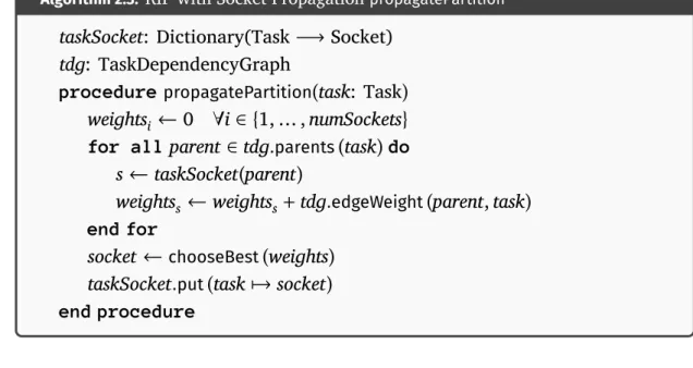
Algorithm 2.3: RIP with Socket PropagationpropagatePartition taskSocket: Dictionary(Task ⟶Socket)

tdg: TaskDependencyGraph

procedure propagatePartition(task: Task)

weights_i ←0 ∀i∈ {1, … ,numSockets}

for allparent ∈ tdg.parents(task)do s← taskSocket(parent)

weights_s ←weights_s+tdg.edgeWeight(parent,task)

end for

socket ← chooseBest(weights)

taskSocket.put(task↦socket)

end procedure initial window window window intersection intersection window initialisation tasks remaining tasks

Figure 2.3:Small drawing showing the options for RIP with Moving Window

Once the partitioner finishes its job, the old-est tasks are flushed from the graph and a new subgraph starts getting built. The user can set up the window size, an initial extra amount of tasks for the first window and the size of the intersection between two consecut-ive windows. This intersection is considered to allow the graph partitioner to exploit the already made partitions to generate the new ones, which is an optimization that aims at reducing the overhead and keeping the data locality whenever it is possible. Figure 2.3 shows a very high level diagram of these op-tions.

2.3.4 Benefits of graph partitioning

While simple heuristics based on round-robin approaches (e.g., DEP) are able to produce optimal partitions in some scenarios, in some other cases they fail in optimally partitioning the graph. In these scenarios, policies based on graph par-titioning clearly outperform simple round-robin approaches.

(29)

2.3 Runtime Informed Partitioning (RIP)

FIFO optimal DEP RIP-DEP

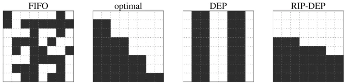
Figure 2.4:Task assignments into two sockets on the first iteration of the Gauss-Seidel method applied to a8×8grid.

As an example, we consider the stationary heat diffusion problem using the it-erative Gauss-Seidel method with a 4-element stencil (top, bottom, left, right) in an8×8regular grid, which corresponds to the the Gauss-Seidel application later described in section 3.1.5. Each task operates over one cell of the grid. In each it-eration, computations over every cell depend on the data of the four neighbouring cells, and the algorithm execution follows a wavefront scheme in the direction of the main diagonal, exploiting the fact that the tasks in the same anti-diagonal are independent between them. For that reason, when targeting two sockets, the op-timal partition consists in dividing the domain along the main diagonal, so at each instant half of the anti-diagonal can be executed in a different socket but main-taining locality as much as possible. This can be seen in figure 2.4, which also shows the different partitions that each approach has produced over the first iter-ation of the Gauss-Seidel method. The specific details on how the graph partition is carried out are explained in section 3.1.4.

We can compare this optimal division with those obtained with a round-robin of stride 2 (DEP) and using graph partitioning (RIP-DEP). For the first case, which follows a round-robin approach, we do not get a partition close to the optimal one. There is a column set to one socket before the stride 2 round-robin distribu-tion since there are some control tasks not shown in the physical domain that are assigned in the same socket as first column’s tasks. In the second case, RIP-DEP makes a division which is much more similar to the optimal one. Finally, the FIFO scheduler distributes the tasks in a complete domain-oblivious way, as we can also see in figure 2.4.

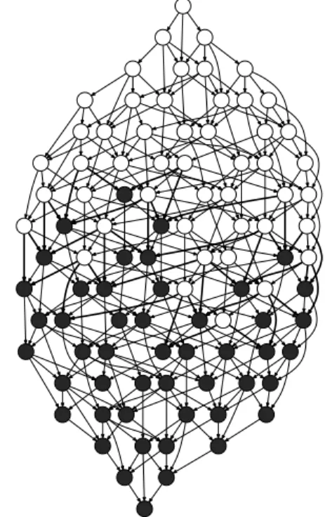
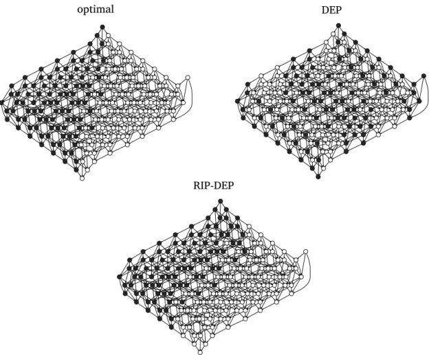
In figure 2.5 we show these partitions expressed at the TDG level on three it-erations of the Gauss-Seidel application (section 3.1.5). The representation of the FIFO scheduler partition is omitted due to its lack of interest since tasks are just

(30)

randomly assigned to one of the two sockets. It is clear that data transfers between tasks assigned to different sockets are minimised in the optimal partition and the one obtained via graph partitioning (RIP-DEP). In contrast, the DEP approach pro-duces a sub-optimal graph partition. The implications of these partitions in terms of the total performance of the Gauss-Seidel application are detailedly commented in section 3.2.

optimal DEP

RIP-DEP

Figure 2.5:Task dependency graph corresponding to three iterations of the Gauss-Seidel code and its optimal partition plus the ones achieved by the DEP and RIP-DEP techniques in a two-socket system.

(31)

3 Experiments

3.1 Experimental environment

3.1.1 Software environment

In all cases, we use the OmpSs [18] toolsuite with a customised Nanos++ v0.9 runtime system and the Mercurium 1.99.9 (rev. 627c863) compiler. For the in-strumentation and analysis of the results we use Extrae 3.2.1 and Paraver 4.5 [7]. OmpSs is a forerunner of the OpenMP task execution model and we will con-sider them as equivalent in our work. In the case of programs using the Lin-ear Algebra Package (LAPACK), we use the open-source implementation from OpenBLAS 0.2.15 [31], [45] compiled for each architecture. Threading of the library is disabled so as not to interfere with Nanos++.

3.1.2 Considered platforms

To evaluate the usefulness of the proposed techniques, we consider three different platforms:

Intel Sandy Bridge

We make use of a single node in a large scale HPC facility. Each node has two 8-core Intel Xeon E5-2760 CPU (Sandy Bridge) at 2.6 GHzwith 20 MB of shared last-level cache and Hyper-Threading disabled, and 8 DIMM of4 GBDDR3 RAM at

1600 MHz. The facility is composed of IBM System X server iDataPlex dx360 M4

nodes interconnected with InfiniBand Mellanox FDR10. It uses IBM LSF queue sys-tem for scheduling the jobs, allowing exclusive use of the requested computation node. We use GCC version 4.8.2 as the backend compiler for Mercurium.

SGI UV100

This is an SGI Altix UltraViolet 100 machine with 3 individual rack units (IRUs) interconnected with NUMAlink at 15 GB/s. Each IRU contains two IP93 blades with two 8-core Intel Xeon E7-8837 CPU (Westmere-EX) at 2.66 GHz and 24 MB

(32)

of shared last-level cache, and 16 DIMM of16 GB DDR3 RAM at 1066 MHz. We use GCC version 4.8.2 as the backend compiler for Mercurium.

IBM POWER8

This is an IBM Power System S824L (8247-42L) machine with two sockets com-posed of two 6-core POWER8 chips, called chiplets, running at 3 GHzand up to 8 threads per core. This is the scale-out version of the POWER8 system, which means that the two chiplets in a socket neither share the last-level cache nor the memory controller (i.e., each chiplet has its own NUMA node). Each chip has a

48 MB shared L3 cache with non-uniform access times, and 16 CDIMM of 64 GB

RAM at1600 MHz. For the experiments, we limit the use of hardware threads to one per core. We use GCC version 4.9.3 as the backend compiler for Mercurium.

3.1.3 Memory latency characterisation of the platforms

Table 3.1:NUMA distances obtained using the numactl --hardwarecommand.

machine chiplet socket node system

Intel Sandy Bridge − 10 11 −

SGI UV100 − 10 13 40/48

IBM POWER8 10 20 40 −

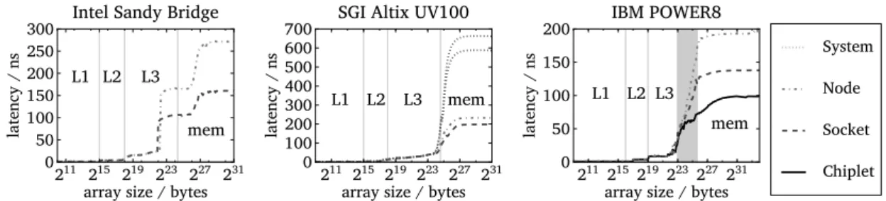
Information regarding the NUMA to-pology of a system is typically avail-able to the runtime system from the firmware via the OS. The numactl --hardware command displays the information the OS provides regard-ing NUMA distances within the system. Table 3.1 summarises the obtained NUMA distances. Besides this information, we measure the real latencies when mov-ing data across the different NUMA domains in the evaluated platforms. We use

lat_mem_rdtool from LMbench [27] to measure the real latencies. These results are shown in figure 3.1. In the case of the Intel Sandy Bridge system, there is an average68% latency penalty in accessing the remote NUMA region memory. In the case of the IBM POWER8, accesses to the memory of the other chiplet located in the same socket suffer from40% latency penalty, while accessing the memory of the remote socket increases the penalty up to 95%. In the case of the SGI UV100, accesses within the same blade have an increased latency of 17% com-pared to accessing the local memory, while there is a significant latency penalty of 3× to access data in other IRUs, or even close to 3.4× in the distant sockets. As shown in figure 3.1, these latencies follow the same pattern and similar ratios as the data obtained from the firmware displayed in table 3.1, except in the case

(33)

3.1 Experimental environment

211 ₂15 ₂19 ₂23 ₂27 ₂31 array size / bytes 0 50 100 150 200 250 300 latency / ns _{L1 L2 L3} mem Intel Sandy Bridge

211 ₂15 ₂19 ₂23 ₂27 ₂31 array size / bytes 0 100 200 300 400 500 600 700 latency / ns L1 L2 L3 mem SGI Altix UV100

211₂15₂19₂23₂27₂31 array size / bytes 0 50 100 150 200 latency / ns L1 L2 L3 mem IBM POWER8 System Node Socket Chiplet

Figure 3.1:Measured memory latencies (in nanoseconds) as we increase the working set size with LMbenchlat_mem_rd.

of the IBM POWER8, where the firmware annotations are not consistent with the real measurements and the proportions in the firmware are the double of the real ones.

3.1.4 Graph partitioning

For partitioning the graphs, we use the methods available in the Scotch 6.0.4 [36] graph partitioning library. When using Scotch, it is possible to partition the graph into k equal parts or to map the graph to a target graph with k vertices. The second option is of much more interest, since it allows to specify the different NUMA distances in the target architecture in order to help the partitioner to group the tasks in the correct way. We represent the target architecture as a complete graph with as many vertices as cores, and with edge distances related to the NUMA distances obtained from the firmware as explained in section 3.1.3. Then, after doing the mapping of the tasks to the target architecture, we assign each task to the NUMA domain where the assigned core resides. For the TDG describing the application, we use the total amount of transferred data between the tasks to give a weight to the edges.

3.1.5 Tested applications

Conjugate gradient

CG is an iterative method for solving linear systems of equations with a symmetric positive-definite matrix. We use a sparse matrix version with a task decomposition as described by Jaulmes et al. [22]. The source code level annotations to guide the NUMA-aware scheduling assign tasks to sockets in a round-robin fashion.

(34)

Gauss-Seidel

This is an algorithm solving the stationary heat diffusion problem using the iter-ative Gauss-Seidel method with a 4-element stencil (top, bottom, left, right). The implementation is based on the available one from BAR [8], with a task decom-position given by tiles but with a modified data allocation strategy to make the tile contents contiguous in memory instead of the rows. The graph follows a wave-front shape, as shown in figure 2.1. The source code level annotations defining the optimal NUMA-aware scheduling are optimised for two sockets and follow a division along the main diagonal of the stencil.

Integral histogram

This algorithm computes a cumulative histogram for each pixel of an image, using a cross-weave scan as described by Porikli [38]. We use a modified version (to use aligned allocations) from the one available in BAR [8]. The halos are allocated in a round-robin fashion, the image data and scan tasks are assigned to a socket in round-robin using the column identifier.

Jacobi

This application solves the stationary heat diffusion problem using the iterative Jacobi method with a similar implementation to the Charm++ project [20], [23]. This implementation uses a 5-element stencil (top, bottom, left, right, centre) and a task decomposition given by blocks of rows. The source code level annotations for assign the blocks of rows to a socket follow a round-robin approach. The double-buffer nature of Jacobi gives an embarrassingly parallel algorithm inside every iteration. Together with the highly symmetric shape of the task dependency graph, it becomes simple to partition, in contrast to the Gauss-Seidel code that solves the same problem.

NStream

NStream is a synthetic benchmark to measure memory bandwidth from the Intel Parallel Research Kernels benchmark suite [43] based on STREAM by McCalpin [28]. We use a task-based implementation ported to OmpSs. Since it works with

(35)

3.1 Experimental environment the operations done, its task graph is made of isomorphic connected components, so partitioning it should be as easy as assigning every component to one socket. Due to the simplicity of the graph, the benchmark gives a good way to detect strange behaviour in the partitioner. The user-level annotations for the NUMA-aware scheduler assign each array to a socket following a round-robin approach.

QR factorisation

Given a general matrix A, a QR factorisation of A is a product A = Q Rwhere Q

is orthogonal and R is upper triangular. We use a task-based implementation of the tiled algorithm described by Buttariet al. [12], that saves the Rmatrix in the upper-triangular part of Aand the Householder reflectors that allow to compute

Q in the lower-triangular part. It uses procedures from LAPACK as kernels for the computations. The source code level annotations assign the blocks of the matrix in a round-robin approach using the row identifier, while the subsequent tasks are assigned where most blocks reside (using the row identifier).

Red-Black

This is the third and last algorithm solving the stationary heat diffusion problem. The data decomposition is exactly the same as for Gauss-Seidel, but the task graph is more similar to Jacobi; the red sub-iterations are embarrassingly parallel (by tiles) and so are the black sub-iterations. The source code level annotations split tasks by following a division along the main diagonal of the stencil.

Symmetric matrix inversion

This algorithm is used to compute the inverse of a symmetric matrix in a fast way by means of a Cholesky decomposition. We use the tiled task decomposition of the dense linear algebra version as described by Al-Omairy et al. [30], and compare our results against the NUMA-aware scheduling. It uses procedures from LAPACK as kernels for the computations. The user-level annotations for the NUMA-aware scheduler assign tasks in a round-robin approach as proposed in that same article.

(36)

3.2 Evaluation

In this section we evaluate the performance of the proposed mechanisms consid-ering the 7 applications and 3 platforms described in section 3.1. Our evaluation considers six different approaches:

• First-In First-Out (FIFO) task scheduler that is unaware of data location. This is the baseline scheduler.

• Socket Aware (SA) scheduler, which is driven by annotations at the source code level. The specific annotations of each benchmark are explained in section 3.1.5.

• The four approaches described in chapter 2: DEP, DEP, SP and RIP-MW. In the case of DEP, we use a stride of2.

For each application, platform and method we repeat each experiment 10 times. In all speedup plots shown in this section, bars are averaged among the different repetitions and normalised to the baseline FIFO scheduler. Bar height represents the mean value, a horizontal thick line is the median, and error bars show the standard deviation of the 10 repetitions. Our experiments run on 16 cores when considering the Sandy Bridge system, on 16 cores when running on the UV100 (a total of 8 cores per socket considering runs on 2 sockets) and on 24 cores in the POWER8 (6 per chiplet, using 4 chiplets). For each system configuration we include a plot of the geometric mean computed over all the executions done con-sidering the 7 benchmarks.

3.2.1 Intel Sandy Bridge

Figure 3.2 shows the execution time speedups when applying the different schedul-ing methods to executions on the Intel Sandy Bridge machine. Average results are also included, using the geometric mean of individual results. SA achieves an av-erage1.16× speedup, while DEP reaches1.14×. RIP schedulers show more vari-ability in their behaviour. RIP-DEP achieves very competitive results, reaching average1.12×speedups. In contrast, RIP-SP is competitive for half of the bench-marks, and suffers significant slowdowns in three benchmarks (CG, QR and SMI). Consequently, average performance is degraded (although the average median is

(37)

3.2 Evaluation Conjugate gradient 0.50 0.75 1.00 1.25 1.50 speed u p

Gauss-Seidel Integral histogram Jacobi NStream

QR factorisation 0.50 0.75 1.00 1.25 1.50 speed u p

Red-Black Symm. mat. inv. 0.50 Geometric mean 0.75

1.00 1.25 1.50

FIFO SA DEP RIP-DEP RIP-SP RIP-MW

Figure 3.2:Speedup results when running on a 2-socket 8-core Intel Sandy Bridge platform.

still above FIFO). Finally, RIP-MW does not reach the speedups of DEP or RIP-DEP in any benchmark due to the overhead of periodically repartitioning the TDG. As a result, an average10% slowdown is obtained.

Individual results per benchmark follow similar trends and are coherent with the different latencies shown in figure 3.1. In the case of CG, the matrix is divided into blocks that are allocated in both NUMA regions. The number of matrix blocks is 30, two less than the double of the number of threads, to make sure there are enough parallel tasks to achieve good performance on 16 cores. While all the con-sidered approaches allocate approximately half of the matrix on each region, the FIFO scheduler is not aware of this situation and it sometimes assigns tasks to the wrong socket. The SA approach based on source code annotations always manages to execute tasks to the right socket. The DEP approach applies a simple modulo function to initialisation tasks and then tasks execute on the socket where more data has been initialised. As a result, DEP attains a significant 1.42× speedup. In case of RIP-DEP each socket seems to get specialised in executing a certain kind of tasks, getting a 1.34× speedup. Finally, RIP-SP and RIP-MW fail in providing significant benefits due to the wrong task placement decisions in the first case and the large overhead of the multiple graph partitions performed by the second. In the case of the exact numerical algorithms QR and SMI, the RIP methods do not improve the performance of the baseline FIFO scheduler since these two bench-marks show very low sensitivity to NUMA effects when using only two sockets, especially if they have similar latencies [30].

Interestingly, in case of the Gauss-Seidel and Red-Black applications, the DEP approach fails in emulating the speedups of1.11× achieved by the SA approach,

(38)

which is guided by user code annotations. In contrast, the RIP-DEP approach does indeed achieve good speedups (1.07×) since its initial graph partition defines a task to sockets mapping very close to the one defined at the application source code level, as shown in figures 2.4 and 2.5. The RIP-SP and RIP-MW techniques fail in providing significant benefits. Although they start from the same good partition as RIP-DEP, the propagation performed by RIP-SP is flawed and the high overhead of RIP-MW undermines its performance.

3.2.2 SGI Altix UV100

Conjugate gradient 0.5 1.0 1.5 2.0 2.5 3.0 speed u p

QR factorisation 0.5 1.0 1.5 2.0 2.5 3.0 speed u p

1.5 2.0 2.5 3.0

4.1 4.1 4.1 3.3 3.3 3.3 3.3

Figure 3.3:Speedup results in the SGI UV100 using 2 sockets.

For the SGI Altix UV100 machine, we have done experiments using two sockets with results visible in figure 3.3. We do not have support to run our executions in isolation in this system, which sometimes adds noise to our experiments. On average, DEP achieves speedups of1.98×over the FIFO approach, while RIP-DEP, RIP-SP and RIP-MW achieve improvements of 2.02×, 1.28× and 1.09× respect-ively. As figure 3.3 shows, some of our methods match or in certain cases outper-form the speedup obtained by the partition designed by the programmer, which is expressed under the SA category.

The strong NUMA effects of the Altix system, described in section 3.1.3, allow the RIP-DEP technique to clearly beat the DEP approach on average due to the excellent speedups it achieves when dealing with the Gauss-Seidel and the Red-Black applications. The DEP technique, based on simple round-robin policies, is

(39)

3.2 Evaluation not able to emulate the optimal partition expressed at the application source level. In contrast, the partition obtained by RIP-DEP is close to the best possible one, which allows the RIP-DEP technique to achieve speedups of2.01×in Gauss-Seidel and 2.08× in Red-Black, very close to the ones achieved by SA, which is 2.05×

faster than FIFO in both cases.

3.2.3 IBM POWER8 Conjugate gradient 0.50 0.75 1.00 1.25 1.50 speed u p

QR factorisation 0.50 0.75 1.00 1.25 1.50 speed u p

1.00 1.25 1.50

2.0 2.0 2.0 2.0

Figure 3.4:Speedup results in the IBM POWER8.

In the IBM POWER8 machine, we run tests on the four chiplets. Results are shown in figure 3.4. In this occasion, DEP reaches a speedup of 1.20×, doubling the 1.10× speedup of SA, while RIP-DEP goes up to 1.11×. On the other hand, RIP-SP and RIP-MW have around a20% performance loss.

Contrary to the good results achieved by the RIP-DEP approach in applications like CG and Integral Histogram seen in the Intel or the Altix platforms, in the POWER8 the RIP-DEP method does not show much performance. This is caused by the inaccurate NUMA distances set in the firmware of the machine as section 3.1.3 describes in detail. Since the graph partitioning performed by RIP-DEP is fed by the firmware NUMA distances, the final partition is suboptimal.

The case for Jacobi, on the other hand, is that our methods surpass the results of the manual partition using the socket-aware scheduler. As we explained in sec-tion 3.1.5, the manual partisec-tion done by the programmer is using a simple round-robin approach, assigning every block of rows and their corresponding tasks to a

(40)

different socket. DEP outperforms the SA techniques by applying a round-robin task distribution of stride 2. Interestingly, RIP-DEP achieves the same perform-ance as DEP without the need for setting up the round robin stride parameter, which highlights the benefits of graph partitioning approaches over DEP and SA.

Regarding the Gauss-Seidel and Red-Black benchmarks, the manual partition using the socket-aware scheduler is optimised for two NUMA regions, as explained in section 3.1.5. For this reason, DEP has a much better performance than SA in these applications even if the partition is not perfect, and this shows our proposals are more prepared for future many-socket scenarios.

3.2.4 Sensitivity to the window size

100 150 200 250 300 350 400 450 # tasks in the window

0.95 1.00 1.05 1.10 1.15 1.20 1.25 1.30 speedup

Figure 3.5:Sensitivity of Jacobi to the win-dow size using RIP-DEP in the In-tel Sandy Bridge when using 150

blocks of rows.

Figure 3.6:Load imbalance problems when choosing an inadequate window size. Dashed tasks and edges are not in the window, colours show the partition.

The window size parameter, corresponding to the number of tasks in the subgraph as introduced in section 2.3, is fundamental for all the RIP methods. For iterative al-gorithms, such as the solvers for the heat diffusion problem or CG, a good window is obtained by selecting a number of tasks of around 2 or 3 whole iterations (plus the ini-tialisation tasks), with an intersection of one iteration for RIP-MW. For dense exact lin-ear algebra applications, the optimal win-dow size is around 2 or 3 times the total num-ber of matrix blocks and an intersection of a couple of complete rows. In all cases, setting up a good window size does not require a deep understanding of the application source code, just a high-level idea of what the al-gorithm does.

Figure 3.5 shows how the window size af-fects the performance of Jacobi when using the RIP-DEP approach with150blocks. We can see how after having150tasks, one for each block, in the window the bene-fits of RIP-DEP over FIFO decrease. The reason is that up until then all tasks tasks are for initialising the data and the task graph is completely disconnected. This

(41)

3.2 Evaluation works fine because, by default, when there is no more information the Scotch library tries to group the vertices in the same order as their identifiers, given by the creation order, which corresponds to consecutive blocks of the stencil, so locality is preserved.

After the initial152tasks (2of them are for setting the borders of the problem), the following 150 tasks carry out the computations of the first iteration of the algorithm, one per block, so when not taking into account all the tasks of the iteration the partitioner is forced to map the connected tasks to the same socket and put the rest freely. For the first iteration, when using two sockets the worst case is when only1/3of the iteration is on the window, because then those tasks and the initializers of the data corresponding to their blocks get to one socket, and the rest to the other. This is seen precisely in figure 3.6, where the stencil is divided into 12 blocks and we get 4 blocks in one part and 8 in the other (plus one border in each part), thus creating a considerably high load imbalance.

In general, the RIP approaches require a window size that is large enough to be representative of the whole parallel run. However, if the windows size is too large, the partition of the initial subgraph becomes too costly, which undermines the benefits of the RIP technique.

3.2.5 Work stealing

Work stealing is an effective technique to improve the performance of parallel applications [3], [4], [39], [47]. Figure 3.7 compares the benefits of all the tech-niques considered in this paper with (grey) and without (white) work stealing when run on the Intel Sandy Bridge and the SGI Altix UV100 using two sockets. The results for the IBM POWER8 are similar to those of the Sandy Bridge. Results appearing in white in figure 3.7 correspond to the ones appearing in figures 3.2 and 3.3.

System-wise, we can see how work stealing provides better results when ap-plied on the Sandy Bridge system than on the SGI UV100. The reason is the large memory latency of the latter system, which hides the benefits of stealing work between sockets. Technique-wise, we see in figure 3.7 how work stealing under-mines the benefits of the SA and DEP techniques, specially when run on the UV100 System. Since these two techniques already provide well balanced task schedules, adding work stealing to them does not add any benefit and, contrarily, forces some

(42)

SGI Altix UV100 (2 sockets) 0.5 1.0 1.5 2.0 2.5 speed u p

Intel Sandy Bridge 0.875 1.000 1.125 1.250 speed u p

Figure 3.7:Benefits over the FIFO scheduler without applying work stealing (white) and with work stealing (shaded in grey). Values are the geometric means for the applications presented in section 3.1.5.

tasks to run on sockets that are far from the data they need. The RIP-DEP tech-nique gets its performance slightly improved by stealing tasks between sockets when running on the Sandy Bridge system and gets its performance degraded on the UV100. These observations indicate small load imbalances with a minimal im-pact on the final performance. The benefits of fixing these imbalances are hidden on the SGI Altix UV100 by the slowdowns due to wrong task scheduling decisions. In all the considered scenarios RIP-SP performs better with work stealing, which indicates that this technique suffers from large load imbalances that undermine its effectiveness.

(43)

Final words

In this work we have shown how graph partitioning methods can increase the performance of parallel applications by mitigating NUMA effects, and it is in fact the first work to present results in a multi-socket cache-coherent NUMA system. In various cases, the benefit of using graph partitioning is on par with a manual mapping of the work to the sockets of a shared-memory node, but without the need for specific annotations at the source code level to guide the scheduling decisions. The benefits of using these techniques are not only so from a theoretical point of view, we have done tests on multiple real-life machines which have made the approach look highly promising.

Graph partitioning is more difficult to use with exact linear algebra algorithms and other applications that do not have an iterative flow, due to their ever-changing structure, not so predictable. In these cases, work stealing can help to improve the performance when compared to blind assignments not taking into account the structure of the program.

To improve the partition, future work can go in the direction of taking even more advantage of the structure of the graph. Indeed, the partitioner can be ex-tended to get better performance with RIP-MW, which should be the way to go with applications that change behaviour during the execution. We expect that the overhead associated with RIP-MW can be reduced with some sort of hard-ware support, following the path set by the Runtime-Ahard-ware Architectures point of view [13], [42]. In this way, RIP-MW can be improved to produce high quality graph partitions under a very low cost. Another proposal for future work consists in applying the partition at the core level, and not at the NUMA region level. This idea aims to get benefit of the data locality within private caches, although the overhead of partitioning is probably higher than just partitioning at the NUMA domain level.

(44)

(45)

Glossary

execution model specification of how a program execution should take place.

processing element one of the basic execution units in a computer, such as a Cent-ral Processing Unit (CPU).

round-robin assignment done in circular order.

runtime system piece of software that implements part of the execution model, controls and carries over the execution of a program.

task in a task-based programming model, portion of a program that is executed sequentially and is considered a unit.

task-based programming model test.

work-stealing scheduling option in which a processing element can execute work from another intended to be executed by another processing element.

(46)

(47)

Acronyms

API Application Programming Interface.

CPU Central Processing Unit.

DEP Dependency Easy Placement.

EFT Earliest Finish Time.

FIFO First-In First-Out.

HPC High Performance Computing.

IRU individual rack unit.

LAPACK Linear Algebra Package.

LLC Last-Level Cache.

NUMA Non-Uniform Memory Access.

RAW read-after-write.

RIP Runtime Informed Partitioning.

RIP-DEP RIP with Dependency Easy Placement.

RIP-MW RIP with Moving Window.

RIP-SP RIP with Socket Propagation.

TDG Task Dependency Graph.

WAR write-after-read.

(48)

(49)

List of Tables

3.1 NUMA distances obtained using the numactl --hardware com-mand. . . 20

(50)

(51)

List of Figures

1.1 NUMA topology with two pairs of sockets generated using lstopo

from hwloc. . . 1

1.2 Task dependency graph for algorithm 1.1 . . . 4

2.1 Partition of the Gauss-Seidel TDG as an undirected graph . . . 13

2.2 Theold dependencies option includes the dashed edges to help the partitioning library. . . 13

2.3 Small drawing showing the options for RIP with Moving Window . 16 2.4 Task assignments into two sockets on the first iteration of the Gauss-Seidel method applied to a 8×8grid. . . 17

2.5 Task dependency graph of Gauss-Seidel and three different partitions 18 3.1 Measured memory latencies (in nanoseconds) as we increase the working set size with LMbenchlat_mem_rd. . . 21

3.2 Speedup results when running on a 2-socket 8-core Intel Sandy Bridge platform. . . 25

3.3 Speedup results in the SGI UV100 using 2 sockets. . . 26

3.4 Speedup results in the IBM POWER8. . . 27

3.5 Sensitivity of Jacobi to the window size . . . 28

3.6 Load imbalance problems when choosing an inadequate window size. Dashed tasks and edges are not in the window, colours show the partition. . . 28

3.7 Benefits over the FIFO scheduler with and without applying work stealing . . . 30

(52)

(53)

List of Algorithms

1.1 Small task-based program . . . 3

2.1 Dependency Easy Placement . . . 12

2.2 Runtime Informed Partitioning . . . 14

(54)

Graph partitioning for the reduction of data transfer in task-based programming models

Master of Science in

Advanced Mathematics and

Mathematical Engineering

M

A

ST

ER

’S

D

EG

R

EE

TH

ES

IS

Graph partitioning for the reduction of data

transfer in task-based programming models

Master’s degree thesis

Author:

Isaac Sánchez Barrera

Advisors:

Marc Casas Guix

Miquel Moretó Planas

Facultat de Matemàtiques i Estadística

Universitat Politècnica de Catalunya

RoMoL Project

Acknowledgements

Contents

1 Introduction

1.1 Problem background

1.2 Task-based parallelism and its opportunities in NUMA

systems

1.3 Graph partitioning

2 Exploiting the task dependency graph

to mitigate NUMA effects

2.1 Dependency Easy Placement (DEP)

2.2 Considerations about applying graph partitioning

algorithms to applications’ TDGs

2.3 Runtime Informed Partitioning (RIP)

3 Experiments

3.1 Experimental environment

3.2 Evaluation

Final words

Glossary

Acronyms

List of Tables

List of Figures

List of Algorithms