Blockmodeling Techniques for Complex Networks.

(1)

Blockmodeling techniques for complex networks

by

Brian Joseph Ball

A dissertation submitted in partial fulfillment of the requirements for the degree of

Doctor of Philosophy (Physics)

in The University of Michigan 2014

Doctoral Committee:

Professor Mark E. Newman, Chair Professor Charles R. Doering

Associate Professor Elizaveta Levina Assistant Professor Xiaoming Mao Professor Michal R. Zochowski

(2)

c

(3)

(4)

ACKNOWLEDGEMENTS

I would like to thank everyone who has helped make this dissertation a reality, starting with my advisor, Dr. Mark Newman. Mark’s extraordinary passion and curiosity have been an inspiration to me. His vast knowledge and patience have been invaluable to my education and professional development. I would also like to thank Dr. Charles Doering, Dr. Elizaveta Levina, Dr. Xiaoming Mao, and Dr. Michal Zochowski, who have kindly taken the time to serve on my dissertation committee.

I would also like to thank Dr. Jean Krisch, who has helped mentor me and guide my career since before I came to Michigan as a freshman. Her wisdom and genuine concern for my success have been a strong positive influence throughout my time here.

Special thanks go to all of my officemates in 320 West Hall, including Brian Karrer, Travis Martin, and Thomas Zhang, who somehow managed to put up with me on a daily basis. It was a pleasure working with such intelligent people with whom I could work and share ideas. My cohort members Jax Sanders and Adam Sypniewski also deserve thanks for their friendship and fresh perspectives in many discussions. I would also like to thank all of my friends from my church’s graduate student and young professional group. I would never have made it this far without their encouragement and support.

Finally, I give my biggest thanks to my parents, to whom I owe everything. This work uses data from Add Health, a program project designed by J. Richard Udry, Peter S. Bearman, and Kathleen Mullan Harris, and funded by a grant P01–

(5)

HD31921 from the National Institute of Child Health and Human Development, with cooperative funding from 17 other agencies. Special acknowledgment is due Ronald R. Rindfuss and Barbara Entwisle for assistance in the original design. Per-sons interested in obtaining data files from Add Health should contact Add Health, Carolina Population Center, 123 W. Franklin Street, Chapel Hill, NC 27516–2524 ([email protected]).

(6)

LIST OF FIGURES

Figure

1.1 (a) The K¨onigsberg bridge problem. The goal is to cross each of the yellow bridges exactly once. (b) The picture rewritten as a network where the vertices are the land and the edges are the bridges. No Eulerian path exists in this network. . . 3 1.2 Jacob Moreno’s sociogram [98]. The triangles are boys and the circles

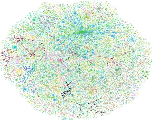
are girls. There are many interactions between boys and between girls, but only a single case where a boy interacted with a girl. . . . 4 1.3 Visualization of the internet taken on June 29, 1999, colored by IP

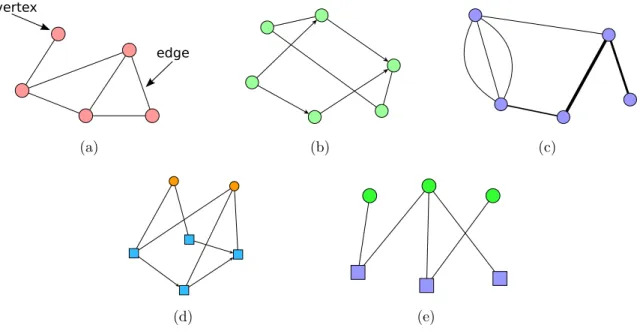
address. Credit for the image goes to Hal Burch and Bill Cheswick of the Internet Mapping Project [23]. . . 7 1.4 (a) Demonstrating a simple network. (b) A network with both

di-rected edges (drawn with an arrow to indicate direction) and undi-rected edges. (c) A network exhibiting both multi-edges and weighted edges (drawn as thickness). (d) A network with multiple kinds of ver-tices. Connection patterns will be specified by the network – here the blue squares form a directed graph on their own, and the orange cir-cles are only allowed to connect to blue squares and in an undirected fashion. (e) Bipartite network, a special case of the type of network shown in (d). . . 9 1.5 A network (a) and its corresponding adjacency matrix (b)

demon-strating both directed and undirected edges as well as a self-edge. . 11 1.6 Example of a network with communities. The vertices are colored

(9)

2.1 Results from the three sets of synthetic tests described in the text. Each data point is averaged over 100 networks. Twenty random ini-tializations of the variables were used for each network and the run giving the highest value of the log-likelihood was taken as the final result. In each panel the black curve shows the fraction of vertices as-signed to the correct communities by the algorithm, while the lighter curve is the Jaccard index for the vertices in the overlap. Error bars are smaller than the points in all cases. . . 43 2.2 Overlapping communities in (a) the karate club network of [152] and

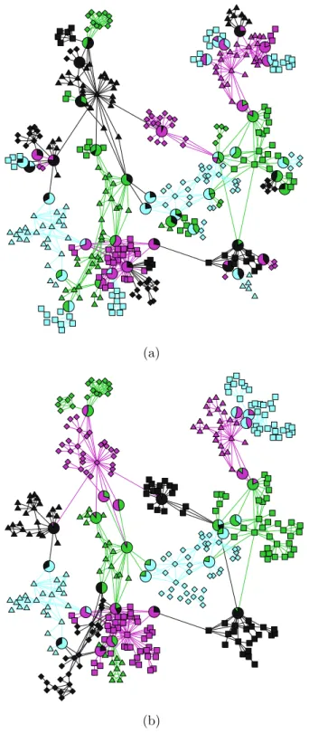
(b) the network of characters from Les Mis´erables [85], as calculated using the algorithm described in this chapter. The edge colors corre-spond to the highest value of qij(u) for the given edge, while vertex

colors indicate the fraction of incident edges that fall in each com-munity. For vertices in more than one community the vertices are drawn larger for clarity and divided into pie charts representing their division among communities. . . 47 2.3 Overlapping communities in the network of US passenger air

trans-portation. The three communities produced by the calculation cor-respond roughly to the east and west coasts of the country and Alaska. 48 2.4 Overlapping communities in the collaboration network of network

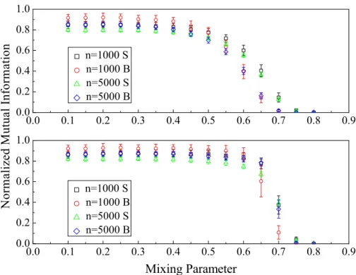
scientists as calculated by the algorithm of Section 2.4 (a) without the post-processing step that ensures connected communities and (b) with the post-processing. Each community is represented as a shape/color combination, except for overlapping vertices, which are always drawn as circles. . . 50 2.5 Performance of the nonoverlapping community algorithm described

in the text when applied to synthetic networks generated using the LFR benchmark model of Lancichinetti et al. [86]. Parameters used are the same as in Ref. [86] and (S) and (B) denote networks with the “small” and “big” community sizes used by the same authors. The top and bottom panels respectively show the results without and with post-processing to optimize the value of the log-likelihood. Ten random initializations of the variables were used for each network and each point is an average over 100 networks. . . 53

(10)

2.6 Non-overlapping communities found in the US college football net-work of Ref. [58]. The clusters of vertices represent the communities found by the algorithm, while the vertex shape and color combina-tion represents the “conferences” into which the colleges are formally divided. As we can see, the algorithm in this case extracts the known conference structure perfectly. (The square black vertices represent independent colleges that belong to no conference.) . . . 54 3.1 Communities in a network demonstrated in the form of a Venn

dia-gram. The test is to assume 2 communities are in the network and extract 3 communities. (a) The community structure. From left to right, the blue community was split into blue and green communities. Colors are additive for overlaps – for example, a vertex in the red and blue communities falls in the purple segment. (b) The first case from list 1. Any vertices belonging to the community set highlighted in blue count for the heuristic. (c) The second case from list 1. Any vertices in the community set highlighted in blue that are extracted as belonging to any of the red sets are counted. More complicated situations can arise when 3 or more communities are present in the network. . . 63 3.2 Twice the change in log-likelihood normalized by the number of

ver-tices betweenK communities andK−1 communities plotted against

K. The stopping point for each network is when it falls below the green line (Wilks’ Theorem prediction). Black circles are the aver-age and standard deviation of the actual data, and red squares are our prediction based on the heuristic described in the text. AIC’s stopping criterion is not drawn, but would be a horizontal line at 2.0. 67 3.3 (a) Histogram of the computed change in log-likelihood when K = 4

for the test described in the text. The red curve is the best fit to a

χ2 _{distribution normalized to match the histogram, and is obviously}

too wide. (b) Corresponding Q-Q plot. The green line is a fit to the quantiles, and the blue line is the liney=x. The fit is good, meaning the shape of the distribution is approximately correct, but the blue and green lines don’t match up, which means that the width of the distribution is incorrect. . . 69

(11)

3.4 Comparison of the two tests mentioned in the text. As in figure 3.2, black squares are the results of the first test, with equal-sized com-munities, and the green line is the stopping point. Blue diamonds are the results of the test with differently-sized communities. The two tests do not have a strong overlap, showing that a network’s commu-nity structure impacts the change in log-likelihood. K = 1,2 are not shown since they actually exhibit community structure – we have no reason to believe that the two tests should give the same change in log-likelihood there anyways. . . 70 3.5 Community structure as extracted using the overlapping community

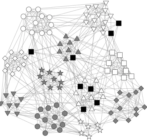
detection blockmodel with AIC (a) and our counting heuristic with a p-value of 0.5 (b). Colored circles correspond to the groups, and the actual conferences are shown by the underlayed grayscale shapes. Extracted communities are correlated with the conference structure in both cases, but AIC doesn’t find the correct number of conferences whereas our heuristic does. See figure 2.6 for a clear version of the actual conferences. Of special interest are the independent teams, drawn as black squares. . . 72 4.1 Probability that an author wrote more than a given number of papers.

Red circles indicate values calculated from the full data set; black squares are values from the data set after papers with fifty or more authors have been removed. The plot is cut off around 500 papers because there is very little data beyond this point. . . 79 4.2 Fraction of papers written by the most prolific authors (with credit

for multi-author papers divided among coauthors, as described in the text). The red (grey) curve represents values calculated from the full data set; the black curve represents values after papers with fifty or more authors have been removed. Note that the two curves are almost indistinguishable. The dashed line indicates the form the curve would take if all authors published the same number of papers. 81 4.3 Number of papers published in each five-year block. Red circles

in-dicate numbers calculated from the full data set; black squares are calculated from the data set after papers with fifty or more authors have been removed. Note that the two values are almost indistin-guishable. The straight line is the best-fit exponential. . . 82

(12)

4.4 Number of unique authors who published a paper in each five-year block. Red circles indicate numbers calculated from the full data set, while black squares are calculated from the data set after papers with fifty or more authors have been removed. Note that the two values are almost indistinguishable. The straight line is the best-fit exponential. . . 83 4.5 Number of authors per paper averaged over five-year blocks. Red

circles indicate the full data set; black squares are the data set after papers with fifty or more authors have been removed. . . 84 4.6 Average number of unique coauthors of an author, averaged in

five-year blocks. Red circles indicate the full data set; black squares are the data set after papers with fifty or more authors have been removed. 85 4.7 Average numbers of citations made (black squares) and received (red

circles) per paper, in five-year blocks. . . 86 4.8 Fraction of citations made more than a given number of years after

publication. Black diamonds include all citations, blue squares are self-citations, red circles are co-author citations, and green triangles are distant citations. . . 89 4.9 Fraction of citations made, by type, in five-year blocks. There were

no citations made in the 1890–1894 block. Blue squares represent self-citations, red circles are co-author citations, and green triangles are distant citations. . . 90 4.10 Probability of future coauthorship with another author as a function

of the number of shared coauthors. The number of shared coauthors is counted at the time of first coauthorship or the date of either coauthor’s last published paper, whichever comes first. . . 94 5.1 (a) Probability of reciprocated friendships as a function of rank

differ-ence (normalized to run from−1 to 1). The histogram shows empir-ical results for a single example network; the solid curve is the fitted function α(z). (b) The equivalent plot for unreciprocated friendships. 108 5.2 The fitted central peak of the friendship probability distributions for

(a) reciprocated and (b) unreciprocated friendships. The horizontal axes are measured in units of absolute (unrescaled) rank difference divided by average network degree. Each blue curve is a network. The bold black curves represent the mean. . . 109

(13)

5.3 The fitted probability function for unreciprocated friendships, minus its central peak. The horizontal axis measures rank difference rescaled to run from −1 to 1. Each blue curve is a network. The bold black curve is the mean. . . 111 5.4 Plots of rescaled rank versus degree, averaged over all individuals

in all networks for (a) in-degree, (b) out-degree, and (c) the sum of degrees. Measurement errors are comparable with or smaller than the sizes of the data points and are not shown. . . 113 5.5 Rescaled rank as a function of school grade, averaged over all

indi-viduals in all schools. . . 114 5.6 A sample network with (rescaled) rank on the vertical axis, vertices

colored according to grade, and undirected edges colored differently from directed edges. Rank is calculated as an average within the Monte Carlo calculation (i.e., an average over the posterior distri-bution of the model), rather than merely the maximum-likelihood ranking. Note the clear correlation between rank and grade in the network. . . 115 E.1 Histogram of the number of papers with a given number of authors.

The vertical line falls at fifty authors and corresponds roughly to the point at which the distribution deviates from the power-law form indicated by the fit. The data for ten authors and more have been binned logarithmically to minimize statistical fluctuations. . . 137

(14)

LIST OF TABLES

Table

4.1 Mean values of some statistics for our data set, with and without papers having over 50 authors. . . 78 4.2 Mean time delay between a paper’s publication date and the dates of

the papers it cites. . . 91 4.3 Percentage of papers that make or receive at least one citation of a

given type. . . 92 B.1 Example networks and running times for each of the three versions

of the overlapping communities algorithm described in the text. The designations “fast” and “naive” refer to the algorithm with and with-out pruning respectively. “Iterations” refers to the total number of iterations for the entire run, not the average number for one ran-dom initialization. “Time” is similarly the total running time for all initializations. Directed networks were symmetrized for these tests. All networks were run with 100 random initializations, except for the LiveJournal network, which was run with 10 random initializations. Calculations were run on one core of a 4-core 3.2 GHz Intel Core i5 CPU with 4 GB memory under the Red Hat Enterprise Linux oper-ating system. Running times do not include the additional cluster aggregation process described in Section 2.5.2, but in practice the extra time for this process is negligible. . . 127

(15)

LIST OF APPENDICES

Appendix

A. Community detection and statistical text analysis . . . 121

B. Results for running time . . . 125

C. Nonoverlapping communities . . . 128

D. Attainability of the maximal solution . . . 132

(16)

CHAPTER I

Introduction

The word “network” has become pervasive in our society. The average person understands that networks are found almost everywhere and will immediately pro-duce such examples as the internet or social networks like Facebook. Pressed a little harder, people can come up with other examples, like the power grid, food webs, and cell phone networks. What most people do not realize however, is that while these networks are different, there is a single set of mathematics that scientists use to describe all of them that unifies them together as networks. This combined un-derstanding is the result of discovering a common thread through years of work from scientists in unrelated fields studying seemingly unrelated topics; each of the examples above and in fact all networks stem from the same building blocks, a set of objects (vertices) and connections between them (edges). The result of this perspective is a powerful tool with far-ranging applications.

The first chapter of this dissertation begins by providing background into the subject of networks. Section 1.1 discusses the many histories of networks and how they came together. This leads to section 1.2, which talks about why physicists are interested in networks, their main contributions to the field, and how they are necessary for the continued success in the modern world of networks. Section 1.3 discusses all of the network basics relevant to the dissertation. This introductory

(17)

chapter wraps up in section 1.4 with the novel contributions of this dissertation to network science and a summary of the main chapters of the dissertation.

1.1 Historical interest

The first interest in networks developed from the mathematical study of graph theory. One of the best known early problems that sparked interest in the field came from Leonhard Euler’s 1735 study of bridges in the Prussian city of K¨onigsberg. The problem posed was this: how could a person cross each of the seven bridges in the city, situated over the Pregel River, without crossing the same bridge twice? This problem is demonstrated in figure 1.1a. Euler’s genius was to acknowledge that the shapes of the landmasses were irrelevant – all that mattered was which landmasses were connected by the bridges. The entire problem can be reduced to traversing edges on a graph, shown in figure 1.1b (not surprisingly, this problem is now in general referred to as finding an Eulerian path), and Euler showed that in the case of the K¨onigsberg bridges, there is no solution.

While graph theory has been around since Euler’s time, its primary focus has been purely mathematical – there has been very little application to real-world networks. Sociologists independently started gaining interest in networks in the early 20th cen-tury. An important example is Jacob Moreno’s 1934 study of school children on the playground [98]. He drew a picture of the children and their interactions, shown in figure 1.2, which he termed a “sociogram”, where the students were represented as triangles and circles for boys and girls respectively and a line was drawn between two students if they were seen interacting on the playground. From this picture, it was easy to see patterns in the interactions, specifically that the boys and girls pri-marily interacted within their own groups. Sociologists quickly saw the use of such pictures and modes of thinking and have been applying and studying social networks ever since. Of particular note are two specific models, the blockmodel and a tiered

(18)

(a)

(b)

Figure 1.1: (a) The K¨onigsberg bridge problem. The goal is to cross each of the yellow bridges exactly once. (b) The picture rewritten as a network where the vertices are the land and the edges are the bridges. No Eulerian path exists in this network.

(19)

Figure 1.2: Jacob Moreno’s sociogram [98]. The triangles are boys and the circles are girls. There are many interactions between boys and between girls, but only a single case where a boy interacted with a girl.

ranking model. In the blockmodel, the ideal situation is that everyone in a particular social clique connects to everyone else within the clique and connects to no one else1_.

Homans’ tiered directed model was based upon an idea of social status where a person is allowed to connect to other people at their same level as well as make connections up the tiers, but is prohibited from connecting to a lower level [35, 75].

The two disciplines listed above are the forerunners of networks as a field. Many different scientific disciplines have contributed to the field, too numerous to discuss here, except to mention the contributions from computer scientists and biologists. One of the questions that attracted computer scientists’ interest in the field was a problem mathematicians had studied for years, the traveling salesman. In this prob-lem, a salesman attempts to travel between several cities. The roads between each

(20)

city have an associated cost of time and effort, and the salesman’s goal is to mini-mize the total cost. This and several other problems united computer scientists and their computational complexity theory with networks [81]. The work done was espe-cially relevant in a practical sense given the parallel development of local computer networks and the much larger connecting network, now known as the internet. Vul-nerabilities in this new physical network were a real issue – scientists needed to be certain that any two computers could communicate with each other even as some connections failed, and that making the connection would be efficient with respect to the network. The main contributions of computer scientists to the early networks literature were minimum cut/maximum flow algorithms and minimum spanning trees (via path distance) in the form of local routing approximation algorithms [40, 53, 93]. A different topic that should also receive mention are computer scientists’ work in classification with an emphasis on natural language and image processing that has applications to networks [19, 68, 69, 70, 88, 121].

Biologists on the other hand became interested in food webs and more recently metabolic and neural networks [31, 147]. Every ecosystem has a network where or-ganisms with a higher so-called trophic level eat oror-ganisms with lower trophic levels, creating a chain connecting the lowest trophic levels up to the highest ones. These networks tell biologists about the stability of an ecosystem and thus are of central interest to ecologists. Similarly metabolic and neural networks are central to un-derstanding how a particular organism works, so they have also received a lot of attention.

Since the early 1990s, the unification of all these different representations and applications became the field of network theory, with the review by Wasserman and Faust playing a significant part [143], and is largely due in part to the involvement of physicists and computer scientists.

(21)

1.2 Interest to physicists

Traditionally, networks were small systems of interacting agents [75, 85, 152]. Re-searchers studying the systems were generally interested in small scale features, on the order of individual node properties. For example, a scientist might ask how im-portant a particular vertex is to the network, often answered in the form of centrality or connectivity measures [143]. However, with the advent of large scale computing and tools such as the internet, it became significantly easier to gather a large data set. Up to that point, a “large” network would be one with one or a few hundred agents. It was now possible to have data sets numbering in the millions and billions of agents. Rather than having specialized knowledge about each actor and interaction in the network, researchers could now only afford to have global knowledge about the entire system. Questions that had been central to networks in the past became dif-ficult to interpret because the amount of information about individual agents got to be too large to handle. Even visual checks for interesting features are difficult, as can be demonstrated by comparing Moreno’s sociogram and the internet2_{, in figures 1.2}

and 1.3 respectively.

Physicists are already well-acquainted with the problems associated with large datasets. On the experimental side, high energy physics experiments are, as of 2013, able to gather terabytes of data each day even after throwing away a significant frac-tion of the data. Dealing with large amounts of data can be a technical challenge, and physicists are better acquainted than most with this problem. From a theo-retical standpoint, large systems are the routine study of statistical physics, which focuses on extremely large numbers of interacting particles. An early use of statistical methods in physics was the application of statistical mechanics to thermodynamics, which deals with physical properties of materials and fluids. One research topic in

2_{Technically this is not a full representation of the internet, but rather a subset of the edges}

defined by a minimum distance spanning tree as measured by route tracing from a single source computer [23].

(22)

Figure 1.3: Visualization of the internet taken on June 29, 1999, colored by IP ad-dress. Credit for the image goes to Hal Burch and Bill Cheswick of the Internet Mapping Project [23].

(23)

statistical physics of particular interest to this dissertation is the interaction of par-ticle spin systems in crystals, famously receiving attention from Ernst Ising in the 1920s [78, 116]. This is an important physics topic since spins affect the electro-magnetic properties of a material. Crystals are defined as having a regular, strongly defined pattern of connections known as a lattice. In that regard, they can be viewed as being well-behaved networks. Between the wide availability of data from an abun-dance of sources (including but not limited to the examples given in section 1.1) and already being interested in similar problems, the expansion of physicists’ interests to include studying networks was a natural one.

1.3 Basics of network structure

In general, a network is a collection of objects, known as vertices, nodes, or actors, and connections (typically pairwise) between them, called edges, as demonstrated in figure 1.4a [106]. There are many different ways these can manifest. For example, edges can be either directed or undirected (fig. 1.4b). There can also be multiple edges between the same pair of vertices, known as a multi-edge, or they can potentially have weights on them (fig. 1.4c). A network with no multi-edges or self-edges (an edge from a vertex to itself) is called simple. It is also possible to have multiple kinds of vertices and edges (fig. 1.4d). A special case of these multi-modal networks are bipartite networks, where there are two kinds of vertices that are allowed to connect to each other but not to vertices of their own type (fig. 1.4e). Every bit of understanding that can be achieved with networks builds off these concepts, so this section will cover the mathematics associated with these concepts and begin extending ideas about connection patterns as a prelude to the rest of the dissertation. The work presented here primarily uses unipartite networks (networks with only a single kind of vertex), but bipartite networks will also be discussed when necessary, so that it is not confusing when they come up in later chapters.

(24)

vertex

edge

(a) (b) (c)

(d) (e)

Figure 1.4: (a) Demonstrating a simple network. (b) A network with both directed edges (drawn with an arrow to indicate direction) and undirected edges. (c) A network exhibiting both multi-edges and weighted edges (drawn as thickness). (d) A network with multiple kinds of vertices. Connection patterns will be specified by the network – here the blue squares form a directed graph on their own, and the orange circles are only allowed to connect to blue squares and in an undirected fashion. (e) Bipartite network, a special case of the type of network shown in (d).

(25)

1.3.1 Adjacency matrix

The most common (and arguably most useful from a theoretical standpoint) math-ematical way of describing a network, denoted G (for graph), is with the adjacency matrix [106]. For a network with n vertices, the adjacency matrix A is an n× n

matrix where each row and column correspond to a particular vertex, and the par-ticular elements correspond to the edges between the vertices. In the bipartite case,

A is called the incidence matrix. The rows and columns correspond to the different kinds of vertices, so A is only square if there are equal numbers of the two kinds of vertices. Aij = 1 means that there is an edge from the jth vertex to the ith vertex,

and takes value 0 if no such edge exists. In the case of a weighted or multi-edge, Aij

takes value of the weight of the edge or number of edges respectively3. For undirected edges, Aij =Aji, and if the network is directed and it is the case thatAij =Aji, the

edge is called reciprocated. By convention, an undirected self-edge takes the value 2 rather than 1, so that the number of ends of edges in the network is preserved when counting the elements of the adjacency matrix. An example of a network and its corresponding adjacency matrix is shown in figure 1.5a and b respectively.

It is common to have a bipartite network yet only be interested in one of the vertex types. In this case, most scientists project the network into a unimodal form, declaring an edge between two vertices if both connect to any of the same vertices in the bipartite case. In terms of the incidence matrix, this means taking the new adjacency matrix to beAAT_or_AT_A_{, where}T_{is the transpose operator, depending on}

which set of vertices is desired in the projection. Additionally, the projected network will often be forced to be simple by dropping all of the self-edges and setting all the remaining positive elements of the adjacency matrix to 1 to eliminate multi-edges.

With the adjacency matrix in hand, other important quantities of the network

3_{Care must be taken here! While weighted and multi-edges are significantly different conceptually}

(26)

(a) A=     0 0 0 1 0 2 1 0 1 1 0 0 1 0 0 0     (b)

Figure 1.5: A network (a) and its corresponding adjacency matrix (b) demonstrating both directed and undirected edges as well as a self-edge.

can be defined. The degree ki of a vertex is the number of ends of edges connected

to vertex i. In terms of the adjacency matrix, ki =P_jAij. Furthermore, since each

edge has 2 ends, the degrees relate to the number of edges m in the network by P

iki = 2m. In directed networks, it is sometimes important to distinguish the

in-and out-degrees: kin_i =P jAij andkiout = P jAji. In this case, P ik in i = P ik out i =m

since the start and end of each edge are distinguishable.

The importance of the degree sequence, defined by the set {ki}, cannot be

un-derstated. A large amount of information in the network is contained in this set. A related yet different concept is the degree distribution, studied by Rapoport and Horvath, which gives the probability that a vertex chosen uniformly at random from the network has a certain degree [124]. In many real-world networks, the degree dis-tribution follows a long-tailed disdis-tribution4 _{[102, 106]. In this case, it is common to}

(27)

have a small fraction of the vertices connecting with a large fraction of the edges, demonstrating the importance of the concept of degree in the network.

By definition of m and n, the average degree in the network hki = 2_nm. The edge density is the fraction of possible edge pairs that are actually edges, i.e. the probability that a randomly chosen vertex pair have an edge: _n₍2_nm₋₁₎. A network is said to be dense if hki = O(n) so that the edge density is a non-vanishing fraction with n. In all other cases, the network is called sparse. It is common to deal with an even more stringent limit, where hki =O(1). Unless otherwise stated, the latter behavior is assumed. When discussing real networks, the network is said to be sparse if hki is only a small fraction of the possible n, since it does not make sense to talk about how the degree is changing with the size of the network given that it is a set size.

1.3.2 Transitivity and clustering

A precursor concept to communities (soon to be described in detail) is the clique. A clique in a network is a group of vertices in which every pair of vertices is connected by an edge (self-edges excluded). In terms of the adjacency matrix, a setC is a clique if for alli, j ∈Cwherei6=j,Aij 6= 0. A clique is considered to be maximal if no other

vertices can be added to the group and still preserve the group’s status as a clique. A different yet relevant concept regarding local graph structure is the neighborhood of a vertex, the set of vertices the vertex is connected to by edges. Many methods for detecting communities are based on these two concepts [9, 112].

Cliques with 3 vertices in them, generally referred to as triangles due to the way they are drawn in a network, hold a special interest for network scientists. A triangle is a potential indicator of transitivity in the network, the concept that the friend of

using this substitution however, as it has been proven that distinguishing a power law distribution from a log-normal distribution can be a difficult task [30]. Deviations at the upper end of the distribution are also observed with regularity so that neither of these distributions are an accurate description over the full range of degrees.

(28)

my friend is also (or should be) my friend. The amount of transitivity in a network is measured by computing the clustering coefficient, C [143, 146]. C is defined as the probability that a randomly selected connected triple (three vertices connected by two edges) is actually a closed triangle, and can be computed either on a vertex by vertex basis or over the entire network. For sparse networks, the density of edges is hki/n, which is small, so it would be reasonable to expect that the clustering should also be small. However, since the 1940s, it has been repeatedly noted that the clustering coefficient takes surprisingly high values in many types of networks, with values as high as 0.3 not uncommon [106, 107, 123]. One idea to explain transitivity in networks is triadic closure, the idea that a triangle became closed because two of the three relevant vertex pairs were already connected [34, 74, 99].

Triangles can also be discussed in a directed graph, but it is much more common to talk about motifs, sometimes referred to as triples in the sociology literature [72, 95, 134]. Historically, sociologists would compare sociograms by computing each of the sixteen possible unique configurations of directed edges, called motifs, between three vertices on the network. These calculations were spurred by a lack of computational power, while still being relatively informative about the network structure5_.

1.3.3 Paths and components

The extension of the concept of neighborhoods in a network is the path. A path is said to exist from vertex i to vertex j if it is possible follow edges in the net-work starting at i and end at j [106]. In terms of the adjacency matrix, a path of length d from i to j is one where there exists some set {l1, l2, . . . , ld−1} such that

Ajl1Al1l2· · ·Ald−2ld−1Ald−1i 6= 0. A path from i to itself is called a cycle. While this

last concept is essentially useless in an undirected network without adding condi-tions about backtracking along edges, it is always non-trivial in directed networks. A

(29)

directed network in which there are no cycles is called a directed acyclic graph. The distance between two vertices is the length of the shortest path between them, which itself is referred to as a geodesic6_. _{The average path length is the}

average distance between vertices in the network. The diameter of the network is the maximum distance taken over all pairs of vertices in the network. The diameter is difficult to compute on large networks, so the average distance is often used as a proxy even though the two can be quite different.

The concept of paths in networks has made it into popular culture. In the late 1960s, a psychologist by the name of Stanley Milgram ran a famous experiment where he asked about 300 residents of Kansas and Nebraska to try to reach a particular friend of his in Boston, with the condition that they were only allowed to forward the letter and directions to a direct acquaintance, who would then continue the chain [94]. Of the forty or so letters that completed the journey, on average they had been forwarded 6.2 times, motivating the popular phrase “six degrees of separation” [145]. Although the methodology in his experiment was questionable (What happened to the letters that did not make it? For the ones that did, did they take the shortest path? What about selection bias in the sample?), many similar results quickly started appearing with other networks [24]. This phenomenon has since been termed the small world effect, which notes that the average path length in a network generally grows slowly with the size of the network [146].

A connected component in a network is the maximal set of vertices where any two vertices have a finite length path between them (in fact, in an undirected network, a vertex that connects to any vertex in the connected component must itself be in the connected component) [106]. Generally there is at most a single connected component that takes up a significant fraction of the vertices in the network, called the giant component, and a number of small components that take varying sizes but

(30)

all scale independently of n [102]. Calculations in this dissertation will typically be restricted to the giant component since it is the most interesting part of the network for the problems discussed.

In a directed network, there are four kinds of partially nested component types. The weakly connected component of a vertex consists of the connected component ignoring edge direction. This contains both the in- and out-components, which are the set of vertices that can reach/be reached by the vertex in question respectively7. The strongly connected component (SCC) is the closest analog of the connected component from the undirected case, which is the set of vertices that can both reach and be reached by other vertices in the SCC – the intersection of the in- and out-components. In other words, for any two vertices in the SCC, there must exist a cycle for one of the vertices that contains the other vertex. As with undirected networks, it is commonly found that there is at most one giant component and many small components, each represented in the form of a bow tie diagram that demonstrates the different component types [22].

1.3.4 Community detection

Continuing the trend of expanding the scale of focus of connection patterns, the scale within a network called the intermediate scale, referred to in Physics as the mesoscopic scale, will be discussed. In real networks, connections between vertices are not random. Vertices have internal characteristics that play into how they connect with their neighbors. A common dynamic in many networks is assortative mixing, sometimes called homophily: actors in the network with a particular property are more likely to connect to others with the same property. For example, students are more likely to be friends with other students of the same age, sex, or race [97, 124].

7_{However, it is incorrect to think of the weakly connected component as the union of the}

in-and out-components, as this does not necessarily include all of the vertices in the weakly connected component.

(31)

When studying networks, the internal mechanisms that generate the network are usually not known, but the effect is seen. Intuitively, the converse of the previous paragraph should be true: the connection patterns should be informative about the vertices in the network, and this is the goal of community detection. For a specific subset of vertices, it is said to be a community if the vertices primarily connect to other vertices within the subset [54, 58]. An example of such a structure is shown in Figure 1.6. While researchers all agree that this structure must be true in a loose sense, the precise definition of a community is subject to much debate [54]. Depend-ing on the context, communities can even be disjoint or overlappDepend-ing. Community structure and the associated network mechanisms is an important topic for network scientists and a lot of work has gone into studying the subject. For the reader inter-ested in the subject who wants significant detail on the problem and the work done to date, Fortunato gives an excellent review of the entire subject in [54].

Figure 1.6: Example of a network with communities. The vertices are colored accord-ing to which of the three separate communities they belong.

There are several early methods for community detection worth mentioning. The first is hierarchical clustering, which arose out of sociological interests. The idea behind hierarchical clustering is that similar vertices (for however similar is defined in the particular context) should slowly aggregate in a pairwise fashion until eventually

(32)

the entire network has aggregated into one single group. Then the objective is to find the right scale at which to stop the agglomeration. Similarly hierarchical clustering can be run by dividing up the network until each vertex is in its own group, which is known as a divisive algorithm. Whether agglomerative or divisive, the full algorithm is represented as a picture in the form of a dendrogram, a form of tree where all the vertices are lined up in a row and connections up the tree show the different agglomeration/division steps. The final cut is a horizontal line where the connections above the line are ignored and the connections below the line form the communities. An example of this technique is the method by Newman and Girvan [108].

The second method is graph partitioning, a method which originated in computer science. The goal of graph partitioning is to minimize the number of edges that run between two groups of a given size, i.e. to find the groups of vertices that require the fewest number of removed edges to create two separate connected components. This is commonly done by computing the Laplacian matrix, a positive semi-definite matrix closely related to the adjacency matrix [29]. The zero eigenvalues of the Laplacian matrix have associated eigenvectors that correspond to the different connected com-ponents of the network. Thus intuitively, two groups of vertices that only have a few edges between them should have a fairly small corresponding eigenvalue, and many graph partitioning methods are based around finding these small eigenvalues [52].

One of the more famous recent measures for community detection is modularity, which grew out of the Girvan-Newman algorithm mentioned above [108]. The idea behind modularity is that two vertices connected by an edge in the same community should get a positive score, but receive a penalty if the two vertices are not connected by an edge, so that a good set of communities gives a high modularity score. The exact amount of penalty can be changed depending on the preferred community structure, but is most commonly taken to be the expected number of edges between the two vertices under the configuration model (to be described in section 1.3.5) so that the

(33)

trivial grouping of the entire network being one community gives a modularity of 0. In this case the expression for modularity can be written asQ= (Aij−

kikj

2m)δ(gi, gj),

where gi is the community of vertex i and δ is the Kronecker delta8.

In an ideal world, it would be possible to find the best modularity score over all combinations of communities, but this has been proven to be difficult [21]. Many computational methods have been devised to approximately maximize modularity, and in practice this measure and the numerous methods do a very good job of finding community structure in networks [54]. Modularity does have a few known problems however, for instance it cannot be used to find very small communities [55], may not have a unique optimum [59], and is somewhat unsatisfactory from a formal view-point [17, 155].

Sometimes it is desired to discuss variants of community structure. As mentioned earlier in the section, there is a problem known as overlapping community detection where vertices are allowed to belong to multiple groups. An early method created for detecting overlapping communities is clique percolation [112]. This method looks for cliques with c vertices in them (where c is an input to the method), and defines two such cliques to be adjacent if they share c−1 vertices. Then a community is the set of vertices that can be reached by traversing adjacent cliques with c vertices as though they were paths. Since a vertex can be in multiple cliques withcvertices that are not necessarily adjacent, this method inherently gives overlapping communities.

Many methods like clique percolation are based on the local structure of the network [9]. These methods are based around growing communities in the network rather than splitting the network up into communities. This has the advantage of finding communities that are compact, connected, and potentially overlapping, several aspects of which are not guaranteed by global methods. The number of communities

8_{Modularity is often written with a normalizing factor of} 1

2mso that it is restricted to run between −1 and 1, although this does not affect the extracted community structure for a given network in any way since it is just a multiplicative constant.

(34)

that local methods find is also dependent on the graph structure rather than being a set number, which could be seen as an advantage or disadvantage depending on the application9_{. It may also be desirable to allow for disassortative structure in}

the community (for example as found in a bipartite network), something which these local methods cannot address. Many of these points will be discussed in further detail throughout this dissertation.

1.3.5 Generative Models

A useful technique in the study of complex networks are generative models, mod-els that can be used to generate synthetic networks [71, 73, 109]. The purpose of using these models is to generate example networks that have particular desirable properties [13, 96, 105, 117, 146]. These can then be used as benchmarks for testing algorithms against or to compare synthetic and real networks.

Many generative models assume that all edges are placed independently10. While realistically this may seem a very poor assumption to make since, as noted earlier in the chapter, there is significant clustering in real networks, it is still possible to get useful information out of the models11_{. Furthermore, this makes the math involved}

more tractable. Throughout the body of this dissertation, this will always be assumed. It is also common to assume the limit of large network size with respect to the vertices, although this assumption will not be the case outside of this section unless stated otherwise.

Historically, one of the simplest, earliest random network model is the Erd˝os-R´enyi random graph, which comes in two flavors [47, 48, 49, 133]. In the first version of

9_{Ideally there should be method that can handle either a fixed or an unknown number of}

com-munities, but little work has been done on this difficult problem [121].

10_{There are a few especially notable exceptions to this. For example, the configuration model [16,}

96, 111] has small correlations between edges. There is also a class of models designed specifically to create networks with non-vanishing clustering. These models place triangles directly into the network instead of edges [105].

11_{This is possibly the most surprising and interesting result to come out of modern statistics, that}

(35)

this model, G(n, p), an edge is placed between each pair of vertices with probability

p, wherep is the same for all vertex pairs. To borrow terminology from physics, this model is a canonical ensemble on the edges, and the second version of the Erd˝os-R´enyi random graph,G(n, m), is the microcanonical ensemble equivalent. G(n, m) generates

m edges and places them uniformly at random over the unique vertex pairs without replacement. In the limit of large network size, these two models are equivalent under the substitution n2p= 2m.

Since edges are placed independently, it is trivial to see that in the Erd˝os-R´enyi model, the expected degree for each vertex is merely hkii=hki=np. As mentioned

in section 1.3.1, the degree sequence is very informative, so this model is not especially realistic12_.

A more realistic model is the well-known configuration model, invented by Malloy and Reed, Bender and Canfield, and many other mathematicians [16, 96, 111]. In this model, the vertices have a given number of edge stubs so as to preserve the degree, and the edges are placed uniformly at random without replacement over the stubs. Thus the probability of an edge between two vertices i and j is kikj

2m where

ki are the parameters of the model and 2m = P_iki by definition, although this is

a misnomer since the graph is not actually generated in this fashion. A modified version of the configuration model with this interpretation in mind was introduced by Chung and Lu [28]. In this version of the model, edges are placed independently between two vertices following a Poisson distribution with mean equal to kikj

2m so that

the degree is preserved only in expectation. In this regard, the degree sequence in this model is analogous to a canonical ensemble from statistical physics compared to the configuration model’s microcanonical ensemble. The advantage of the Chung-Lu model over the configuration model is that it is occasionally easier to deal with it mathematically.

12_{In fact this model is not realistic in a variety of ways. About the only property it does correctly}

(36)

For most probabilistic network models that place edges independently, each edge follows a Bernoulli distribution with probability dictated by the model; simply put, either there is an edge between a pair of vertices or there is not an edge. In some cases, it is more convenient to use the Poisson distribution where the parameter of the distribution, which doubles as the mean, is the same value as the Bernoulli case, where it also doubles as the mean. Technically this creates a multigraph, but for sparse networks the expected number of multi-edges is small, so it is only a minor error. In return, the mathematics can become significantly easier due to the additive property of the Poisson distribution: the sum of two Poisson distributed random variables with meansλ1 and λ2 respectively is Poisson distributed with meanλ1+λ2.

This dissertation will repeatedly take advantage of this formulation.

A common way of generating networks, rather than placing edges probabilistically, is to grow them: the network starts with a small number of vertices, and then more are added and edges are placed between the vertices that exist at each step. A common theory is that some networks follow a rich get richer scheme as they develop, where vertices with a higher degree are more likely to have new edges connect to them [120]. This is commonly thought to be true for citation networks, where it is only possible to cite papers that have already been written and scientists are more likely to cite the famous papers than lesser-known ones in their field. This preferential attachment has been realized in many network models, for example in the famous paper by Barab´asi and Albert [13, 117]. In this model, at each time step, a single vertex gets added to the network and has a set degree. The other ends of the new edges get placed among the existing vertices in proportion to their degree. In particular, this model reproduces a long-tailed degree distribution, a feature observed in real networks [120]. Another common synthetic modeling technique is to start with a network that has a regular structure and move the edges around, called rewiring. One well-known model of this type is the small-world model by Watts and Strogatz [146]. In this

(37)

model, the n vertices each have degree 2k, where the vertices are arranged in a circle and connect to k neighbors on each side. Then with probability p, each edge is removed and placed again uniformly at random over the vertex pairs. Depending on the value of p(and k, albeit in a minor role), the resulting network can have zero or non-zero clustering and exhibits or does not exhibit the small world effect.

With these and many more models, it is possible to calculate all sorts of interesting statistics. However, this dissertation will take a different turn; the main focus is in fitting network models to real networks. Network models are perfect for learning the structure of real networks since they are well-principled – the type of structure the model is looking for can be understood exactly. In particular, since the models presented in this dissertation are probabilistic in nature, the statistics literature can be leveraged against all of these questions. Likelihood maximization methods are a perfect place to start this discussion.

1.3.6 Maximum likelihood estimation

A commonly used method for extracting information from networks by using probabilistic models is maximum likelihood estimation. The idea behind this method is rather simple: maximize the probability (referred to in this sort of posterior case as the likelihood) that the observed graph was generated with respect to the parameters of the model. According to most models, the edges are generated independently, so this will often take the form

P(G|Θ) =Y i<j P(Aij|Θ) Y i P(Aii|Θ) (1.1)

for an undirected network where Θ are the model parameters. The self-edge terms, when allowed as in equation 1.1, are split into a separate term and will look slightly different compared to the other edge terms because of the conventional factors of two

(38)

in the adjacency matrix.

Since the likelihood is a product of a large number of terms, it is more convenient to work with its logarithm, called the log-likelihood, which turns the product into a sum without changing the position of the maximum because the logarithm func-tion is strictly increasing. For simple models, the maximizafunc-tion can be done directly by taking derivatives, setting the expression equal to 0, and solving it in the stan-dard Calculus-based approach. For example, the Erd˝os-R´enyi random graph G(n, p) (ignoring self-edges for simplicity) has likelihood

P(G|Θ) =Y i<j pAij₍₁₋_p₎(1−Aij) (1.2)

where the product only runs over i < j since the model generates undirected graphs. Taking the log of equation 1.2 gives us the log-likelihood

L=X i<j Aijlog(p) + (1−Aij)log(1−p) . (1.3)

Setting the derivative of the log-likelihood with respect to p equal to 0 and solving for pgives the best fit solution:

∂L ∂p = 0 = X i<j Aij p − (1−Aij) 1−p ! 0 = m p − n 2 −m 1−p p=m/ n 2 . (1.4)

Fitting this model to an observed network matches the number of edges to the number observed in the graph (or equivalently matches the average degree) but cannot do anything more complex than that.

(39)

model is fit to data. However, direct maximization alone will not be sufficient for the models presented in this dissertation since, as will be seen in the next section, many of the parameters are discrete, so other methods must be employed to estimate those particular parameters.

1.3.7 Stochastic blockmodels

The natural extension of the previous sections is the family of models known as stochastic blockmodels [131, 142]. In these models, each vertex is assigned to a group, and connect with the other vertices based on these groups. As with other probabilistic network models, the strength of the stochastic blockmodels stems from their rigorous mathematical background. It is possible to prove exactly what kind of structure, community or otherwise, the model is picking out, and when that structure can be found [37, 38]. They also offer a flexibility unrivaled by other methods – since much of the information is encoded by the vertices themselves, they can be used to describe a wide variety of network structures with minimal modification.

An early and particularly simple model in this class is the standard stochastic blockmodel, a community detection model where the probability of an edge between two vertices is given by a mixing matrix, ωgi,gj whose element is determined by the

communities of the two vertices, denoted gi [131, 142]. The name of this model and

the class of models in general is a reference to the sociological model mentioned in section 1.1, although it is clear that this model is significantly more flexible than the earlier one. For example, it can account for both assortative and disassortative structure depending on the elements of the mixing matrix, whether they are strongly diagonal or strongly off-diagonal. However, like the Erd˝os-R´enyi random graph, ver-tices within a group all have the same expected degree. What this means in practice is that if this model is used to find community structure in a real network, the best set of “communities” it finds often correspond to a split between high and low-degree

(40)

vertices [37].

A significantly more useful model is Karrer and Newman’s degree-corrected stochas-tic blockmodel [83]. In this model, every vertex has an additional parameter θi that

controls the degree of the vertex, while retaining the mixing matrixωfrom the earlier model. The probability of an edge between two vertices is θiωgi,gjθj. The additional

flexibility in the form of controlling the degree makes this model much more useful in practice than the standard stochastic blockmodel.

The models discussed in the body of this dissertation are all variants of stochastic blockmodels. The discussion in this section has focused on traditional assortative and disassortative community detection up to this point, but it should be clear that this sort of model can be useful in discovering other structure as well. Such an example will be discussed in depth in chapter V in the form of a mathematical realization of Homans’ ranking model [75].

1.3.8 Expectation-maximization algorithm

As mentioned in section 1.3.6, maximization via derivatives is not sufficient for many network models. To supplement that approach, this dissertation will make extensive use of the maximization technique known as the expectation-maximization (EM) algorithm [39]. The EM algorithm is a technique for maximizing the likelihood of a parameterized latent, that is unobserved, variable model. For stochastic block-models, the latent variables are the communities (or whatever vertex information the model concerns itself with) and the parameters are the mixing matrix and any other relevant parameters explicitly defined in the model. The algorithm is performed by splitting the single maximization into two deterministic steps, which individually can be much simpler to solve than the combined problem. The first (Expectation) step is to find the distribution of the latent variables while holding all other observables and parameters constant, and the second (Maximization) step is to maximize the explicit

(41)

expression with the latent variables over the parameters, a step which is often done directly with derivatives. These two steps are computed in an alternating fashion until the parameters converge, at which point both steps are satisfied simultaneously. The EM algorithm is proven to monotonically increase the likelihood at each step, and converge to a critical point of the likelihood13_{. This critical point is not guaranteed}

to be the absolute maximum, so the algorithm will typically be run multiple times (at different starting locations, since it is deterministic) and the best result kept as the desired answer.

There are many equivalent formulations of the EM algorithm, and two will be presented here which will be useful later in the dissertation. Mathematically the objective is to turn the log of a sum into a sum of logs, since these are much easier to differentiate. A simple and direct way this can appear is via Jensen’s inequality in the form log P uxu ≥X u qulog xu qu , (1.5)

where the xu are some set of positive numbers (which in our case will be related to

the probability of a specific edge) and the qu are any nonnegative numbers satisfying

P

uqu = 1. This statement is a valid application of Jensen’s inequality because the

logarithm function is concave. Notice in particular that the equality can be recovered by making the particular choice

qu =xu/

X

u

xu. (1.6)

It is not immediately clear how thequ correspond to the latent variables of our models,

so this is demonstrated by comparing this method with a second way of writing the

13_{Since each step individually maximizes the log-likelihood with respect to a particular set of}

parameters, it is trivial that the likelihood must increase with each iteration. Furthermore, well-defined likelihoods have an upper bound of 1, so this increase has to stop somewhere. It will soon be shown that where this two-step process converges corresponds to a critical point of the original likelihood.

(42)

EM algorithm:

log(P(G|Θ))≥log(P(G|Θ))−D Q(Z)||P(Z|G,Θ), (1.7)

whereP(G|Θ) is the probability of the data given the parameters (written in a format suggestive to the application towards networks), Z refers to the latent variables, and we’ve introduced Q(Z) as any probability distribution over Z. D(P1(X)||P2(X)) =

P XP1(X)log P1(X) P2(X)

is the Kullback-Leibler divergence (also referred to as the rel-ative entropy) of distributions P1(X) and P2(X) over some random variable X. In

particular, the Kullback-Leibler divergence is weakly greater than 0 and equals 0 if and only if P1(X) = P2(X) almost everywhere14. Thus whereas Q(Z) can be any

probability distribution, the right hand side of equation (1.7) will be maximized (and thus the two sides of the equation will be equal) when Q(Z) = P(Z|G,Θ), the dis-tribution of the latent variables. Simplifying equation (1.7) gives

P(G|Z,Θ) is the form of our model given the latent variables and is much easier to write explicitly than P(G|Θ) since there’s no additional sum over the latent vari-ables. The term P(Z|Θ) is the prior on the latent variables and is often independent compared to the probability of the graph with respect to the parameters and thus maximized separately from the rest of the equation. The two steps of the EM

algo-14_{For the network models, the fact that the Kullback-Leibler divergence is additive over}

(43)

rithm are to computeQ(Z) = P(Z|G,Θ) holdingΘconstant then to maximize equa-tion (1.8) with respect toΘwhile holdingQ(Z) constant. Comparing equations (1.5) and (1.8) with the appropriate substitutions (qu =Q(Z) and xu =P(G, Z|Θ)), it is

clear that the two are equivalent and thus both represent valid EM algorithms. This dissertation will primarily use the Jensen formulation since it will be easier to follow for the models presented.

In most applications of the EM algorithm, the M step becomes easy to compute and a closed form solution is not uncommon. The E step can be another story however. It is rare for this step to have a closed form solution, so a numerical method like Markov Chain Monte Carlo (MCMC) is usually needed to obtain the distribution of the latent variables [127].

1.4 Outline of the dissertation

In this chapter we have given a brief introduction to networks. The techniques discussed will be instrumental in the following chapters. With this dissertation, we expand upon previous work in several key areas of networks, focusing on the use of stochastic modeling techniques. Specifically, we apply techniques previously unseen to networks research and make progress on unanswered questions. We use principled approaches and when possible make rigorous derivations of our methods. The results are useful methods that are effective both in synthetic tests as well as real world networks.

In chapter II, we introduce a stochastic blockmodel for overlapping community detection that can be run in a memory and computationally efficient manner due to both steps of the EM algorithm having closed form solutions. Part of our effort is spent improving upon the efficiency of the implementation, making it useful for detecting community structure even on modern networks numbering in the millions of nodes and edges. We include appendices (A,B,C) tying this model with other

(44)

models both in the networks and computer science literatures, and to demonstrate our implementation’s efficiency. This chapter and associated appendices are based on the work presented in the author’s publication [10].

In chapter III, we create a heuristic that attempts to solve the question of choosing the correct number of communities for the overlapping community detection model introduced in chapter II. This heuristic is based loosely on model selection techniques from Statistics, specifically likelihood ratio tests. Using networks generated according to this community detection model, we show that the heuristic correctly selects the number of communities where other model selection methods fail, and it can also accurately predict the mean of the change in log-likelihoods when comparing the fits for K and K + 1 communities where no more than K communities are present in the network. Furthermore, we demonstrate that this accuracy in selecting the correct number of communities translates over to real networks. This chapter is based on unpublished work.

Chapter IV explores a different topic of interest, multi-modal networks. We an-alyze data from papers published in the American Physical Society journal series Physical Review, taking into account both authors and paper citations. We give spe-cial attention to how authors cite each others’ papers, an analysis that requires both authorship and citation information. This is supplemented by publication date infor-mation, so we also study how these citation patterns have changed over the history of the journals. This temporal discrimination is especially important since the number of publications in the journals is growing exponentially. We discover that a researcher cites his or her own papers and his or her collaborators’ papers a large fraction of the time, but the extent of this has not changed significantly over time. Furthermore, the citations received from collaborators come sooner than researchers not personally known. There is also a large amount of reciprocity; citations from one scientist to another are often returned in the form of citations later on. Transitivity among

(45)

au-thors is large. However, while still significant, triadic closure is only a small part of transitivity on the whole. This chapter is based on the author’s publication [92].

Chapter V focuses on a blockmodel which, instead of use in community detection, is used for rank ordering a network based on global flow of edges. The basic idea is that the type of network we are interested in is structured almost in an acyclic fashion, and we use our model to describe the generative processes involved. We apply this model on a collection of high school friendship networks and show that the networks demonstrate remarkably similar behavior, regardless of the characteristics of the school. The rank of the vertices appear to have a striking resemblance to a measure of popularity or social status within the school, and the pattern of connec-tions qualitatively resembles Homans’ tiered model [75]. This chapter is based on the author’s publication [11].

(46)

CHAPTER II

Overlapping community detection model

2.1 Introduction

In chapter I, we introduced background on community detection methods. We gave two examples of stochastic blockmodels that are used to detect communities in the traditional sense. In this chapter, we attempt to extend these methods to allow for overlapping communities. In a general sense, overlapping communities are significantly more difficult to describe than nonoverlapping communities because of a much larger number of parameters – the models can describe a wider variety of structure. Furthermore, even if you’re able to write down a model, it is possible that you won’t be able to extract any useful information in a reasonable amount of time. One way researchers have worked around this problem is to create methods based on local community structure [9]. Rather than splitting an entire network into com-munities in one step, these methods instead look for local groups within the network, based on analysis of local connection patterns. Methods of this kind give rise natu-rally to overlapping communities when one generates a large number of independent local communities throughout the network. Moreover, the communities tend to be compact and connected subgraphs, a requirement not always met by other methods. On the other hand, global detection methods can capture large-scale network struc-ture better and are more appropriate when particular constraints, such as constraints