White Noise Reduction for Wideband Sensor Array Signal Processing

(1)

White Noise Reduction for Wideband Sensor

Array Signal Processing

Mohammad Reza Anbiyaei

Supervisors:

Dr. Wei Liu and Dr. Xiaoli Chu

Thesis submitted in candidature

for graduating with degree of doctor of philosophy

March 2018

c

(2)

Abstract

The performance of wideband array signal processing algorithms is dependant on the noise level in the system. In this thesis, a method is proposed for reducing the level of white noise in wideband arrays via a judiciously designed spatial transformation followed by a bank of high-pass filters. The method is initially introduced for uniform linear arrays (ULAs) and analysed in detail. The spectrum of the signal and noise after being processed by the proposed noise reduction method is analysed, and the correlation matrix of the processed noise is derived.

The reduced noise level leads to a higher signal-to-noise ratio (SNR) for the system, which can have a significant effect on the performance improvement of various beam-forming methods and other array signal processing applications such as direction of ar-rival (DOA) estimation.

The performance of two well-known beamformers, the reference signal based (RSB) beamformer and the linearly constrained minimum variance (LCMV) beamformer is re-viewed. Then, the theoretical effect of applying the proposed noise reduction method as a pre-processing step on the performance enhancement of RSB and LCMV beamformers is studied. The theoretical results are then confirmed by simulation. As a representative example of wideband DOA estimation application, a compressive sensing-based DOA estimation method is employed to demonstrate the improved estimation by applying the pre-processing noise reduction method, which is confirmed by simulation.

Next, the idea is extended to wideband non-uniform linear arrays (NLAs). Since, NLA does not have a uniform spacing, the beam response of the row vectors of the transfor-mation is distorted. Therefore, the transfortransfor-mation is re-designed using the least squares method to satisfy the band-pass requirements of the transformation. Simulation results show a satisfactory improvement in the the performance of RSB and LCMV beamform-ers for the NLA structure.

(3)

The idea is further extended to uniform rectangular arrays (URAs) and uniform circu-lar arrays (UCAs), as two major types of the planar arrays. Two methods are proposed for reducing the effect of white noise in wideband URAs and for each one, a different trans-formation is designed. The first one is based on a two-dimensional (2D) transtrans-formation and the second one is an adaptation of the method developed for the ULA case. The devel-oped method for the UCA structure is based on a one-dimensional (1D) transformation, with modified modulation for the transformation to satisfy the required band-pass char-acteristics of the transformation. Same as linear array structures, the RSB and LCMV beamformers are used to demonstrate the performance enhancement of the method for planar arrays.

(4)

List of Abbreviations

:

ANC Active Noise Control

CRB Cramer-Rao Bound

CS Compressive Sensing

CSSM Coherent Signal Subspace Method

DFT Discrete Fourier Transform

DTFT Discrete-Time Fourier Transform

DOA Direction of Arrival

ESPRIT Estimation of Signal Parameters via Rotational Invariance Techniques

FFT Fast Fourier Transform

FIR Finite Impulse Response

ISSM Incoherent Signal Subspace Method

LCMV Linearly Constrained Minimum Variance

MSE Mean Square Error

MUSIC MUltiple Signal Classification

NLA Non-uniform Linear Array

NP Non-deterministic Polynomial-time

NR Noise Reduction

PSD Power Spectral Density

RMSE Root Mean Square Error

RSB Reference Signal Based

SBL Sparse Bayesian Learning

SINR Signal-to-Interference plus Noise Ratio

SIR Signal-to-Interference Ratio

SNR Signal-to-Noise Ratio

SRACV Sparse Representation of Array Covariance Vector

(8)

SVD Singular Value Decomposition

TDL Tapped Delay-Line

TOPS Test of Orthogonality of Projected Subspaces method

TSNR Total Signal-to-Noise Ratio

ULA Uniform Linear Array

UCA Uniform Circular Array

URA Uniform Rectangular Array

ZP Zero Phase

(9)

List of Figures

1.1 A simple beamformer with its outputy[n]given by a linear combination of the received array signalsx0[n], x1[n], ···, xM−1[n]weighted with the

coefficientsw0,w1,···,wM−1. . . 5

2.1 A general wideband beamformer withMsensors andJtaps. . . 14

2.2 The RSB adaptive beamforming structure. . . 15

2.3 PSD of the desired signal. . . 18

2.4 The LCMV adaptive beamforming structure. . . 26

2.5 The equivalent single TDL beamformer for LCMV when the desired sig-nal is arriving from broadside. . . 26

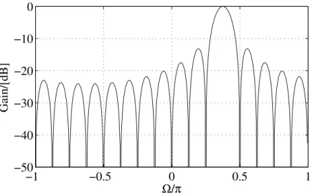
3.1 A block diagram for the general structure of the proposed noise reduction approach. . . 30

3.2 Frequency responses of the row vectors of A in the ideal case and the high-pass filtering effect of a sample row vector. . . 33

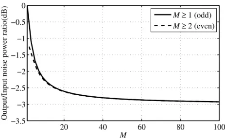
3.3 Output to input noise power ratio for odd (M>1) and even (M>2) values ofM. . . . 37

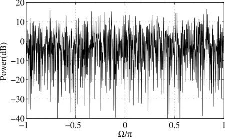
3.4 Power spectrum of the output of the noise reduction system withM=16. . 42

3.5 The frequency response of the 16_×16 DFT matrix. . . 54

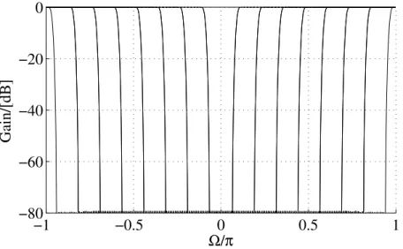
3.6 Frequency response of an example band-pass filter withM=16. . . . 55

(10)

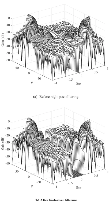
3.7 Frequency response of the resultant beamformer with respect to normalised signal frequency and DOA angle, when applying the filter coefficients in Fig. 3.6 to the received array signal. . . 55 3.8 Frequency response of the 16 linear-phase 101-tap FIR high-pass filters. . 56 3.9 The beam pattern of a sample row vector before and after high-pass

filter-ing (ULA,M=16). . . . 57 3.10 The power spectrum density of the spatially and temporally white noise

before and after processing (M=16). . . 58 3.11 SINR performance of both beamformers with and without the proposed

noise reduction (NR) method (M=16,J=100). . . . 62 3.12 SINR performance of both beamformers with and without the proposed

noise reduction method with regard to input SNR (M=16,J=100). . . . . 63 3.13 DOA estimation results with and without the proposed white noise

reduc-tion. . . 65 3.14 RMSE vs input SNR. . . 66 4.1 Frequency response of the row vectors of the 15_×15 designed

transfor-mation matrix for NLAs. . . 75 4.2 SINR performance of both beamformers with and without the proposed

noise reduction method for the NLA. . . 77 4.3 SINR performance of both beamformers with and without the modified

noise reduction (NR) methods for the NLA. . . 81 5.1 The structure of a URA, where a signal impinges from azimuth angleθ

and elevation angleφ . . . 85 5.2 A block diagram of the proposed noise reduction method based on a 2D

transformation. . . 86 5.3 Frequency responses of the 2D transformation applied to anM_×N URA. 89 5.4 The high-pass filtering effect of the (m,l)-th 2D filter in the ideal case. . . 90

(11)

5.5 The high-pass filtering effect of the (m,l)-th 2D filter in the signal fre-quency domain in the ideal case. . . 90 5.6 The general structure for UCA. . . 96 5.7 Frequency responses of an example 2D-DFT vector and its corresponding

1D-DFT vector, for the directional signal arriving fromθ=90◦andφ=45◦.101 5.8 SINR performance of both beamformers with and without the proposed

noise reduction (NR) methods for the URA. . . 104 5.9 SINR performance of the RSB beamformer with the desired signal

arriv-ing fromθd=5◦andφd=0◦. . . 105

5.10 The beam-pattern of a sample row vector of the transformation designed for UCA, before and after modifying the condition number,M=30,φ =

90◦. . . 107 5.11 SINR performance of both beamformers with and without the modified

noise reduction (NR) methods for the UCA,M=30,J=5. . . 108 6.1 SINR performance of RSB beamformer with NR method and without NR

with equivalent length,l_hp =101. . . 115 6.2 SINR performance of LCMV beamformer with NR method and without

NR with equivalent length,lhp=101. . . 116

6.3 SINR performance of both beamformers with respect to number of taps, with NR method and without NR with equivalent lengthJeq. . . 117

(12)

List of Tables

3.1 MSE for the directional signal. . . 60 3.2 Power loss for the white noise. . . 60 4.1 Sensor locations for the wideband NLA example. . . 74 5.1 MSE for the directional signal before and after the proposed noise

reduc-tion process for different URA sizes. . . 102 6.1 Computational complexity of the noise reduction based implementation,

the RSB and LCMV beamformers. . . 113 6.2 Computation time of the noise reduction based implementation, the RSB

and LCMV beamformers. . . 118

(13)

List of Publications

:

Journal papers:

1. M. R. Anbiyaei, W. Liu, and D. C. McLernon, “ White noise reduc-tion for wideband linear array signal processing”, IET Signal Pro-cessing, DOI: 10.1049/iet-spr.2016.0730, accepted, yet to appear in the printed journal.

Conference papers:

1. M. R. Anbiyaei, W. Liu, and D. C. McLernon, “Performance im-provement for wideband beamforming with white noise reduction based on sparse arrays”, in Proc. 25th European Signal Processing Conference, pp. 2433-2437, Greece, September 2017.

2. M. R. Anbiyaei, W. Liu, and D. C. McLernon, “White noise reduction for wideband beamforming based on uniform rectangular arrays”, in

Proc. 22nd Digital Signal Processing Conference, pp. 1-5, London, UK, August 2017.

3. M. R. Anbiyaei, W. Liu, and D. C. McLernon, “Performance im-provement for wideband DOA estimation with white noise reduction based on uniform linear arrays,” inProc. IEEE, 9th Sensor Array and Multichannel Signal Processing Workshop (SAM), pp. 1-5, Rio de Janeiro, Brazil, July 2016.

(14)

Acknowledgements

:

I would like to take this opportunity to express my deepest gratitude to my supervisor Dr. Wei Liu for his persistent encouragement, guidance and support, and also for giving me the opportunity to pursue my PhD studies under his supervision.

I also thank my second supervisor Dr. Xiaoli Chu for her help and support regarding the doctoral development program.

Finally, I would like to thank my parents for their continuous encour-agement and support.

(15)

Chapter 1 Introduction

1.1 Introduction

Wideband array signal processing, including beamforming and direction of arrival (DOA) estimation, has various applications in radar, sonar and wireless communications, and has been studied extensively in the past.

In [1], different adaptive beamformer methods and parameter estima-tion is reviewed thoroughly. Wei et. al [2] has reviewed different methods of beamforming and array structures. Krim and Vberg review background material and of the basic problem formulation of the parameter estimation in [3]. They introduce spectral-based algorithmic solutions to the signal parameter estimation problem, and the suboptimal solutions are compared to the parametric methods. Allen and Ghavami review the fundamentals of array signal processing in [4], and they review different adaptive beam-forming and estimation methods considering both narrowband and wide-band cases. Some difficulties and practical techniques related to sensor

(16)

1.1. Introduction 2

arrays are addressed in [5]. Such as, placing sensors as an array for accu-rate measurement, calibrating a sensor array by experiment and etc.

The performance of wideband array signal processing algorithms is de-pendent on the level of noise in the system, and normally the lower the level of noise, the better the performance is. Many methods have been developed in the past to reduce the noise level, such as adaptive noise can-cellation (ANC) [6], the Wiener filters [7, 8], and zero phase (ZP) noise re-duction methods [9, 10]. The ANC uses a reference undesired noise source and a primary source contaminated by noise, and then adaptive filtering is employed to produce a cleaned result [11]. The Wiener filter produces an estimate of the desired signal by minimising the mean squared error (MSE) between the noisy signal and a reference [12, 13]. The ANC and Wiener filter methods have proved to work well in specific applications but due to their adaptive nature, they have high computational complexity. ZP noise reducers can reduce the noise without the need to know a priori information of the signal [14,15]. The limitation of ZP noise reducers is that, the signal has to be periodic [16], and it is mainly applied to speech signals. In this thesis, a novel non-adaptive white noise reduction approach is developed with low computational complexity, and relatively good performance, with no limitation on the received wideband signal.

In addition to the wideband beamforming, the wideband DOA estima-tion is also a field of interest in this thesis. Many DOA methods have been proposed for both narrowband and wideband signals, and two

(17)

rep-1.1. Introduction 3

resentative ones are the multiple signal classification (MUSIC) [17] and the estimation of signal parameters via rotational invariance techniques (ESPRIT) [18] algorithms, which were originally proposed for narrow-band signals. For widenarrow-band signals, a commonly used approach is to decompose the wideband signal into different frequency bins and trans-form the wideband problem into a narrowband one through various fo-cusing or interpolation algorithms [19, 20]. In addition, methods such as incoherent signal subspace method (ISSM) [21], coherent signal space method (CSSM) [22] and test of orthogonality of projected sub-spaces method (TOPS) [23] have also been proposed.

Recently, with the development of compressive sensing theory [24, 25], many sparsity based DOA estimation methods were developed. A source localization method based on a sparse representation of sensor measure-ments is introduced in [26]. In [27], a DOA estimation method is proposed based on a novel data model using the concept of a sparse representation of array covariance vectors (SRACV), in which DOA estimation is achieved by jointly finding the sparsest coefficients of the array covariance vectors. The sparse spectrum fitting algorithm for the estimation of DOAs of mul-tiple sources is introduced in [28], and its asymptotic consistency and ef-fective regularization under both asymptotic and finite sample cases are studied. In [29], the authors propose co-prime arrays for effective DOA estimation.

(18)

1.1. Introduction 4

the wideband case. A method named wideband covariance matrix sparse representation (W-CMSR) is proposed in [30]. In this method, the lower left triangular elements of the covariance matrix are aligned to form a new measurement vector, then DOA estimation is achieved by representing this vector on an over-complete dictionary under the constraint of sparsity. In [31], the sparse Bayesian learning (SBL) technique is used to estimate the DOAs of independent narrowband/wideband signals by reconstructing the covariance vectors with high computational efficiency. In [32], a class of low-complexity compressive sensing-based DOA estimation methods for wideband co-prime arrays is proposed, which is based on the narrow-band DOA estimation method for co-prime arrays [29].

Wideband arrays are affected by noise from different sources. These noise sources include the voltages due to thermal noise [33] also known as Johnson-Nyquist noise [34], the shot noise [35], the cosmic black-body radiation [36] and etc. The classical central limit theorem [37] asserts that the distribution of the summation of different random variables converges to a normal, Gaussian distribution with mean 0, which is the definition of the white noise. Therefore, one common assumption for noise in wideband arrays is that it is spatially (and in many cases also temporally) white. That is, the noise at one array sensor is uncorrelated with that at other sensors. Under this assumption, it seems that there is not much can be done about it and simply it has to be accepted whatever is left of the noise component after processing the signals. For example, in the simplest beamforming

(19)

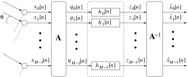
1.1. Introduction 5 0 0 1 1 0 0 1 1 0 0 1 1 000000 000000 000000 000000 000000 000000 111111 111111 111111 111111 111111 111111 00000 00000 00000 00000 00000 11111 11111 11111 11111 11111 000000 111111 00000 00000 00000 00000 00000 00000 11111 11111 11111 11111 11111 11111 y[n] x0[n] w₁ w0 θ _x₁_[_n_] x_M₋₁[n] w_M₋₁

Fig. 1.1: A simple beamformer with its outputy[n]given by a linear combination of the received array signalsx0[n],x1[n],···,xM−1[n]weighted with the coefficientsw0,w1,···, wM₋1.

structure shown in Fig. 1.1, the beamformer output y[n] is a linear combi-nation of the received array signalsx₀[n],x₁[n], _···,x_M₋₁[n]weighted with the coefficients w₀, w₁, _···, w_M₋₁, where n is the discrete time index, M

is the number of sensors in the array and θ is the angle of arrival of the impinging signal. The values of these coefficients are obtained based on some criterion such as maximising the output signal-to-interference plus noise ratio (SINR).

The question here is, whether there is anything that can be done to re-duce the effect of the white noise in a wideband array system (without at-tenuating the directional signals) so that the performance of the subsequent processing (such as DOA estimation and beamforming) can be improved.

In this thesis, the aim is to answer that question by developing a novel method to reduce the white noise level of a wideband array using a

(20)

combi-1.1. Introduction 6

nation of a set of judiciously designed spatial transformations and a bank of high-pass filters, and the key is to realise that the white noise and the direc-tional wideband signals received by the array have different spatial char-acteristics. Based on this difference, and motivated by the low-complexity subband-selective adaptive beamformer proposed in [38], first the received wideband sensor signals is transformed into a new domain where the di-rectional signals are decomposed in such a way that their corresponding outputs are associated with a series of tighter and tighter high-pass spec-tra, while the spectrum of noise still covers the full band from ₋π toπ in the normalised frequency domain. Then, a series of high-pass filters with different cut-off frequencies are applied to selectively remove part of the noise spectrum while keeping the directional signals unchanged. Finally, an inverse transformation is applied to the filtered outputs to recover the original sensor signals, where compared to the original set of received sen-sor signals, the directional signals are left intact while the noise power has been reduced.

One condition placed on the transformation matrix is that it must be invertible. It has been further assumed that it is also unitary and thus the discrete Fourier transform (DFT) matrix is used as a representative exam-ple for the uniform linear array (ULA) case and a least squares based de-sign is introduced for the non-uniform linear array (NLA) case. Detailed analysis shows that the signal-to-noise ratio (SNR) of the array after the proposed processing can be improved by about 3 dB in the ideal case. This

(21)

1.2. Original Contributions 7

is then translated into improved performance for beamforming, as demon-strated by both theoretical analysis and simulation results. This work is fo-cused on two well-known beamformers, namely the reference signal based (RSB) [39, 40], and the linearly constrained minimum variance (LCMV) beamformers [41].

The method is also extended to uniform rectangular arrays (URAs), and uniform circular arrays (UCAs) as examples of planar arrays.

1.2 Original Contributions

The original contributions of this work to the field of array signal process-ing are listed as follows,

• The SNR of the received signal can be improved by a maximum of 3 dB using the proposed noise reduction method for different array structures such as ULA, NLA, URA and UCA which have been pre-sented in this work.

• Using the developed noise reduction method an increased output SINR performance is achieved for the classic RSB and LCMV beamform-ers, for different array structures.

• Simulation results show an improved estimation accuracy for the com-pressive sensing based DOA estimation for the ULA structure.

(22)

reduced computational complexity and more robustness.

• No prior information of the impinging signal is needed and the method is quite flexible. Therefore, it can be used for different array signal processing applications, such as beamforming and DOA estimation. In the following, the contributions of the work are explained in greater detail.

1.2.1 White noise reduction for wideband uniform linear array sig-nal processing with applications in beamforming and DOA es-timation

A novel method is proposed for reducing the level of white noise in wide-band ULAs via a judiciously designed spatial transformation followed by a bank of high-pass filters. 3 dB improvement in total SNR is achieved by this method. A detailed analysis of the method and its effect on the spec-trum of the signal and noise is presented. The reduced noise level leads to a higher SNR for the system, which can have significant effect on the performance of various beamforming methods and other signal processing applications, such as DOA estimation.

The improved performance of two well-known beamformers, namely, the RSB and the LCMV beamformers is analysed. Initially, a detailed theoretical performance analysis is presented, and then, the improved per-formance is confirmed using simulation.

(23)

A compressive sensing based method employing the group sparsity con-cept is employed to analyse the performance improvement for DOA esti-mation. The performance is evaluated by calculating the error between the estimated and the actual DOA angles of the received signals. By apply-ing the noise reduction method, the error between the estimated and the actual DOA angles was reduced. Therefore, the estimation accuracy has been improved by employing the noise reduction method. The improved estimation accuracy is confirmed by simulation.

By studying the structure of the method further, it is understood that if a classic beamformer is applied to a set of array signals which have been processed by the noise reduction method, the pre-processing and the clas-sic beamformer can be modelled as an equivalent beamformer with longer TDLs. Additionally, the complexity of the noise reduction method includ-ing the beamformer part is less than the direct implementation with equiv-alent length. Also, with the noise reduction method, a more robust beam-forming can be achieved, since by using the noise reduction pre-processing the numerical issues due to calculating the optimum beamforming coeffi-cients based on inversion of correlation matrices can be avoided.

1.2.2 Extension of the white noise reduction method for non-uniform linear arrays

The idea is extended to the NLAs by redesigning the transformation using least squares filter design method. Therefore, the noise reduction method

(24)

is adjusted to be applicable to the non-uniform sensor layout of NLAs. A prototype filter using least squares method is designed, and modulated to different frequency subbands to cover the whole normalised spectrum. A low condition number is crucial, to be certain that the transformation is invertible. Initially, the diagonal loading method is used to keep the con-dition number low. Similar to the ULA case, 3 dB improvement in total SNR is achieved, which leads to the performance enhancement for beam-forming. This enhancement is demonstrated by simulation, using RSB and LCMV beamformers.

Also, for reducing the condition number of the designed transforma-tion matrix, a modificatransforma-tion method is proposed based on replacing the small singular values of the transformation. The effect of this modification method on the beam-pattern and the condition number of the transforma-tion is presented, and the beamforming performance of the noise reductransforma-tion method using the modified transformation is investigated using simulation.

1.2.3 Extension of the white noise reduction method for planar ar-rays

The idea is also extended to two major types of planar arrays, namely, URAs and UCAs.

In case of the URA, two design methods are introduced for the noise reduction method, and for each one the transformation is redesigned. The first method is based on a two-dimensional (2D) transformation, and the

(25)

1.3. Outline 11

second one is an adaptation of the ULA noise reduction method, which is based on one-dimensional (1D) transformation of the received signals.

For the UCA case, a 1D transformation is presented, which is almost similar to the ULA case, and the difference is in modulating the prototype filter to different subbands. Due to the sparse nature of circular arrays, the condition number of the transformation might be high, which is in this case, and the condition number is reduced by replacing the small singular values of the transformation, same as in the NLA case.

The effect of the noise reduction methods for the planar arrays on per-formance improvement of RSB and LCMV beamformers is confirmed by simulation.

1.3 Outline

This thesis is organised as follows.

In Chapter 2, the wideband beamforming is briefly reviewed and a de-tailed theoretical performance analysis is provided for the two well-known classic beamformers, namely, RSB and LCMV beamformers. These two beamformers are used for different applications in this thesis.

The white noise reduction method based on the ULA structure is pro-posed in Chapter 3, with a detailed analysis of the spectrum and correla-tion matrix of the noise after the proposed processing, when DFT matrix is used as transformation. Then, the effect of the noise reduction method on

(26)

1.3. Outline 12

the performance enhancement of the RSB and LCMV beamformers and a compressive sensing based DOA estimation is presented, and confirmed by simulation results.

The idea is extended to the structure of the NLAs in Chapter 4. The least squares approach is used for designing the transformation with satisfactory band-pass response.

The idea is further extended to the URA and UCA structures as exam-ples of the planar arrays in Chapter 5, where two methods are presented for the URA case, one based on 2D filtering and one by directly adopting the method developed for the ULA structure. For the UCA case, the mod-ulation of the row vectors of the transformation is modified to satisfy the structure of the UCA.

In Chapter 6, it is shown that the proposed noise reduction method is equivalent to a traditional tapped delay-line (TDL) system. The perfor-mance and computational complexity of the beamformers are compared, with the proposed pre-processing and without any pre-processing with the same length.

Finally, conclusions are drawn in Chapter 7, with possible topics for future work.

(27)

Chapter 2 Adaptive Wideband Beamforming

In this chapter, the general idea of wideband beamforming is briefly re-viewed. The RSB and LCMV beamformers are reviewed as examples for adaptive wideband beamforming, and a detailed analysis of their perfor-mance is provided.

2.1 Wideband Beamforming

For wideband beamforming, a TDL is normally employed, with Fig. 2.1 showing a general structure, where M is the number of sensors, J is the length of the TDL and∆denotes a tapped delay. The coefficient for the m -th sensor at -thek-th position of the TDL is denoted byw_m_,_k,m=0,_···,M₋

1,k=0,_···,J₋1. All J weights at the m-th TDL form anelement weight vector w_m, m = 0,_···,M₋1, and all M element weight vectors form a

MJ_×1total weight vectorw, and they are defined as:

w_m= [w_m_,₀,w_m_,₁,_···,w_m_,_J₋₁]T, (2.1)

(28)

2.1. Wideband Beamforming 14 , , ,0 ,0 ,1 ,1 n M−1 M−1 M−1 w₀ w_{0 −1}_J M−1[n] x ] [ x₀ w w w _J₋₁ ] [ y n w₀

Fig. 2.1: A general wideband beamformer withMsensors andJtaps.

w=

wT₀,wT₁,_···wT_M₋₁T , (2.2) where_{·}T denotes the transpose. The received signal by them-th sensor at the k-th position of the TDL is denoted by x_m_,_k[n], m= 0,_···,M₋1,

k=0,_···,J₋1. All J received signals at the m-th TDL form an element signal vector x_m, m=0,_···,M₋1 and allM element signal vectors form the total input signal vectorx, which are defined as:

x_m=

x_m_,₀[n],x_m_,₁[n],_···,x_m_,_M₋₁[n]T

, (2.3)

x= [xT₀,xT₁,_···,xT_M₋₁]T . (2.4) Finally, the beamformer outputy[n]is given by

y[n] =wTx. (2.5)

The idea is to process the received array signals by the noise reduc-tion method, so that the noise level in the received signals will be reduced. Then, the new set of array signals with reduced noise level will be fed to the

(29)

2.2. Reference Signal Based Adaptive Beamformer 15

+

-+

r[n] e[n] x[n] w y[n]

Fig. 2.2: The RSB adaptive beamforming structure.

following beamformers. In the following, two widely-used adaptive beam-forming methods are briefly reviewed and the theoretical performance re-sults are then derived based on the proposed noise reduction method.

2.2 Reference Signal Based Adaptive Beamformer

The reference signal based (RSB) beamformer is normally employed when a reference signal r[n] is available, where the weight vector of the beam-former can be adjusted to minimise the MSE between the reference signal and the beamformer outputy[n][39, 40], as shown in Fig. 2.2. TheMJ_×1 optimal weight vector is given by:

w_opt =ΦΦΦ_x−1s_d , (2.6)

where_{·}−1 denotes the inverse operator,ΦΦΦ_x is the signal correlation ma-trix with sizeMJ_×MJ, and is defined by:

(30)

where E_{·} denotes the mathematical expectation, _{·}∗ denotes the com-plex conjugate, ands_d is the reference correlation vector with sizeMJ_×1,

s_d =E[x∗r₀[n]] , (2.8)

withr₀[n] being the normalised reference signal with unit power.

There are three components for each of the received sensor signals: de-sired signal x_d[n], interference x_i[n] and noise x_v[n]. The desired signal

x_d[n] is a deterministic signal received from the intended transmitter. The interferencex_i[n]is a deterministic or random signal received by the array transmitted from a source but it does not have the characteristics of the desired signal. The interference can be a deterministic signal transmitted from the same source as the desired signal, which is the case for the multi-path reflection [42]. Otherwise, the source of interference can be from dif-ferent transmitters, which is the case when there are difdif-ferent transmitters in the range. This can happen when multiple transmitters and receivers are trying to communicate in the same area. Also, disturbance signals trans-mitted from the jammers are considered as interference [43]. The jammers may transmit deterministic or random signals to interrupt the communi-cation between the transmitter based on their design. The noise xv[n] is a

random signal which come from different sources such as the voltages due to thermal noise [33] also known as Johnson-Nyquist noise [34], the shot noise [35], the cosmic black-body radiation [36] and etc.

(31)

superpo-2.2. Reference Signal Based Adaptive Beamformer 17

sition of the absorption associated with all the impinging signals and the noise [44, 45]. Therefore, the signal available at the m-th sensor and k-th tap is,

x_m_,_k[n] =x_d_m_,_k[n] +x_i_m_,_k[n] +x_v_m_,_k[n]. (2.9) So, the total signal vectorxcan also be decomposed into three correspond-ing parts:

x=x_d+x_i+x_v. (2.10)

Since the desired signal, interference and noise are independent and so, uncorrelated with each other, ΦΦΦx is also a linear superposition of the

cor-responding parts and can be decomposed into three MJ_×MJ correlation matrices corresponding to the desired signal, interference and white noise components, respectively. i.e.,

Φ

ΦΦ_x =ΦΦΦ_d+ΦΦΦ_i+ΦΦΦ_v. (2.11)

In the following, each of the correlation matrices from (2.11) are deter-mined.

First, the desired signal part is considered. To simplify the theoretical calculations, it is assumed that the desired signal x_d[n] has a flat power spectral density (PSD) equal to 2πp_d/∆ω_d, where p_d, ω_d and∆ω_d are the power, frequency, and bandwidth of the desired signal, respectively. The PSD of the desired signal S_d(ω) is illustrated in Fig. (2.3) with ω₀ being the centre frequency.

(32)

2.2. Reference Signal Based Adaptive Beamformer 18 ω ∆ωd 2πp_d ∆ωd ω0 Sd(ω)

Fig. 2.3: PSD of the desired signal.

of a signal at different times. Therefore, the auto-correlation function of the desired signalx_d[n]is

R_d[τ] =E[x_d[n] x_d[n+τ]] , (2.12) whereτ is the time delay. According to the Wiener-Khinchin theorem [46] the auto-correlation function R_d(τ) is the inverse Fourier transform of the PSD S_d(ω). Therefore, R_d(τ) = 1 2π Z ∆ωd S_d(ω)ejωτdω , (2.13) where j=√₋1.

By taking the inverse Fourier transform fromS_d(ω), the auto-correlation function of the desired signal can be obtained as [40]:

R_d(τ) = p_dsinc ∆ω_dτ 2 ejω0τ _. _(2.14)

(33)

2.2. Reference Signal Based Adaptive Beamformer 19 sub-matrices as: Φ ΦΦ_d =       ΦΦΦ_d₀_,₀ _··· ΦΦΦ_d₀_,_M₋₁ ... . .. ... ΦΦΦ_d_M₋₁_,₀ _··· ΦΦΦ_d_M₋₁_,_M₋₁       , (2.15)

where each correlation sub-matrix is aJ_×Jmatrix and corresponds to the correlation of the desired signal of two different element signal vectors. Therefore, ΦΦΦdm₁,m₂ =E h x∗_d m₁x T dm₂ i . (2.16)

Note that the correlation between the desired signal at the k₁-th tap of the

m₁-th element and thek₂-th tap ofm₂-th element is given by:

h Φ ΦΦ_d_m 1,m2 i k1,k2 =E h x∗_d m₁,k₁[n]xdm₂,k₂[n] i . (2.17)

The desired signal received at them-th element and thek-th tap is a copy of the original desired signal with a delay among the array elements, as well a delay among taps. So

x_d_m_,_k[n] = x_d[n₋mTe−kT0] , (2.18)

where Te is the unit propagation delay between elements, and T0 is the propagation delay between adjacent taps. So, (2.17) can be written as:

h ΦΦΦ_d_m 1,m2 i k1,k2 =R_d[(m₁₋m₂)T_e+ (k₁₋k₂)T₀] . (2.19)

It is assumed that the adjacent array sensor spacing is half a wavelength of the maximum frequencyω_max to avoid the spatial aliasing [47].

(34)

There-2.2. Reference Signal Based Adaptive Beamformer 20

fore, the propagation delay between adjacent sensors can be expressed as

Te = L csin(θd) = π ωmax sin(θ_d), (2.20)

where L is the array spacing, c is the wave propagation speed, and θ_d is the DOA of the desired signal. Next step is to define the delay between two adjacent taps T₀. It is normally assumed that the delay between the adjacent taps is r times the delay associating with a quarter wavelength corresponding to the maximum frequency [48], which is equal to a delay associated with 90◦ phase shift atωmax . Therefore,

T₉₀ = π

2ω_max . (2.21)

So, the delayT₀ can be written as

T₀ =rT₉₀ = πr

2ω_max . (2.22)

Now, from (2.14) and (2.19),

h ΦΦΦ_d_m 1,m2 i k1,k2 = p_dsinc ∆ω_d 2 [(m1−m2)Te+ (k1−k2)T0] ×ejω0[(m1−m2)Te+(k1−k2)T0]_. _(2.23)

For an easier representation, the above equation is simplified by replacing the bandwidth ∆ω_d and centre frequency ω₀ with B_d = ∆ω_d/ω_max and Ω₀ =ω₀/ω_max, respectively. Consequently, the terms∆ω_dT_e andω₀T_e can be written as, ∆ω_dTe = ∆ω_d ωmax πsin(θ_d) =B_dπsin(θ_d), (2.24) ω₀T_e = ω0 ωmax πsin(θ_d) =Ω₀πsin(θ_d). (2.25)

(35)

Similarly,∆ω_dT₀ andω₀T₀ are written as, ∆ω_dT₀ = ∆ωd ω_max · πr 2 =Bd πr 2 , (2.26) ω₀T₀= ω0 ωmax · πr 2 =Ω0 πr 2 . (2.27)

Therefore, in the simplified form, the correlation of the desired signal at the k₁-th tap of the m₁-th element and the k₂-th tap of the m₂-th element can be expressed as,

h Φ ΦΦdm₁,m₂ i k1,k2 = p_dsinc B_d 2 τd ejΩ0τd _, _(2.28) whereτ_d is, τ_d =πh(m₁₋m₂)sin(θ_d) + (k₁₋k₂)r 2 i . (2.29)

Next step is to determine the interference correlation matrix ΦΦΦ_i using the same approach. The DOA θ_i of the interference is different from θ_d. Same as before, to simplify the theoretical calculations, it is been assumed that the interference signal x_i[n] has a flat PSD, equal to 2πp_i/∆ω_i, where

p_i, ω_i and∆ω_i are the power, frequency and bandwidth of the interference signal, respectively. Same as (2.15), the interference correlation matrixΦΦΦi

is separated intoM_×M sub-matrices as:

ΦΦΦi=       Φ ΦΦi0,0 ··· ΦΦΦi0,M−1 ... . . . ... Φ ΦΦiM−1,0 ··· ΦΦΦiM−1,M−1       , (2.30)

where each correlation sub-matrix is a J_×J matrix, corresponding to the correlation of the interference of two different element interference signal

(36)

2.2. Reference Signal Based Adaptive Beamformer 22 vectors, Φ ΦΦim₁,m₂ =E h x∗_i_m 1x T im₂ i . (2.31)

The correlation between the interference at the k₁-th tap of the m₁-th ele-ment and thek₂-th tap of them₂-th element is:

h ΦΦΦim₁,m₂ i k1,k2 =E h x∗_i m₁,k₁[n] xim₂,k₂[n] i . (2.32)

Similar to the desired signal in (2.28), in the simplified form, the correla-tion of the interference at the k₁-th tap of the m₁-th element and the k₂-th tap of them₂-th element can be expressed as:

h ΦΦΦim₁,m₂ i k1,k2 = p_isinc B_i 2 τi ejΩ0τi _, _(2.33) whereB_i=∆ω_i/ω₀ andτ_i is τi=π h (m₁₋m₂)sin(θi) + (k1−k2) r 2 i . (2.34)

Since it is assumed that the noise available at each sensor is temporally and also spatially white, so the noise is mathematically independent be-tween the sensors in the TDL. Therefore, the noise correlation products of the correlation matrix in (2.11) are zero, apart from the product of the same delay-line. Similar to (2.15) and (2.30), the noise correlation matrixΦΦΦv is

also separated intoM_×M sub-matrices, so:

ΦΦΦv =          Φ ΦΦv0,0 0 ··· 0 0 ΦΦΦv1,1 ··· 0 ... ... . .. ... 0 0 _··· ΦΦΦvM₋1,M₋1          , (2.35)

(37)

where each non-zero noise correlation sub-matrix is a J_×J matrix. It is assumed the white noise has a flat PSD equal to 2πσ2

v/∆ωv, where σv2 is

the noise variance and ∆ω_v is the bandwidth of the noise. Therefore, as in (2.28) and (2.33), the correlation of the noise at the k₁-th and k₂-th tap of the samem₁-th element is

[ΦΦΦ_v_m 1,m1]k1,k2 =σ 2 v sinc B_v 2 τv ejΩ0τv_, _(2.36) whereBv =∆ωv/ω0 andτv is τv=π h (k₁₋k₂)r 2 i . (2.37)

Finally, the reference correlation vector s_d is determined. Assuming the reference signalr_o[n]is the same as the desired signalx_d[n], s_d in (2.8) can be written as

s_d =E[x∗r_o[n]] = E[x∗x_d_o[n]]. (2.38) wherex_d_o[n]is the same asx_d[n], with unit power. It has been assumed that the desired signal, interferences and the noise are uncorrelated with each other. Therefore, (2.38) can be expressed as:

s_d =E[x∗_dx_d_o[n]]. (2.39) Furthermore,s_d can be expanded as:

s_d =

s_d₀_,₀,_···,s_d₀_,_J₋₁,_···,s_d_M₋₁_,₀,_···,s_d_M₋₁_,_J₋₁T, (2.40) wheres_d_m_,_k, m=0,_···,M₋1, k=0,_···,J₋1, indicates the correlation of the reference and the desired signal at them-th element andk-th tap, given

(38)

2.2. Reference Signal Based Adaptive Beamformer 24 by: s_d_m_,_k =√p_dsinc B_d 2 τs ejΩ0τs_, _(2.41) with τ_s =πhmsin(θ_d) +kr 2 i . (2.42)

SinceΦΦΦx and sd are fully determined, using (2.6), wopt can be calculated

for the RSB beamformer.

The beamformer output can be calculated from (2.5), and the output power is: P= 1 2E h ky[n]_k2₂i= 1 2w H optΦΦΦxwopt, (2.43)

where _{k · k}₂ is the l₂ norm and _{·}H denotes the Hermitian transpose. As denoted in (2.11), ΦΦΦx can be expressed as desired, interference and noise

parts. Therefore, the output power can also be expressed as:

P_d = 1 2w H optΦΦΦdwopt, (2.44) P_i= 1 2w H optΦΦΦiwopt, (2.45) P_v = 1 2w H optΦΦΦvwopt. (2.46)

Finally, the output SINR of the beamformer is:

SINR= Pd

Pi+Pv

. (2.47)

(39)

2.3. Linearly Constrained Minimum Variance Adaptive Beamformer 25

2.3 Linearly Constrained Minimum Variance Adaptive

Beamformer

In practice, the reference signal r[n] may be unavailable. However, when some information on the DOAs as well as the bandwidth limits of the de-sired signal and/or the interferences is available, a linearly constrained minimum variance (LCMV) beamformer can be employed for effective beamforming [2, 49].

min

w w

H_Φ_Φ_Φ

xw subject to CHw=f, (2.48)

where w and ΦΦΦ_x are defined as before in Section 2.2, C is the MJ_×J

constraint matrix and f is the J_×1 response vector. The beamformer will always have the desired response set out by the constraint equationCHw= f, no matter how the weights are adjusted. The structure of the LCMV beamformer is shown in Fig. 2.4. The solution to (2.48) can be obtained using the Lagrange multipliers method [49],

w_opt =ΦΦΦ−_x1C(CHΦΦΦ−_x1C)−1f. (2.49) The correlation matrixΦΦΦ_x is determined in the same way as in Sec. 2.2. So, only the constraint matrix C and the response vector f need to be de-fined. In the following, Cand f are defined for the case when the desired signal is coming from the broadside, i.e.,θ_d =0◦.

In this case, the desired signal components are received at the same time at the array elements, and so there would be no delay between the

(40)

2.3. Linearly Constrained Minimum Variance Adaptive Beamformer 26

x[n]

y[n]

CHw=f w

Fig. 2.4: The LCMV adaptive beamforming structure.

ˆ wM−1[n] x0[n] ˆ w0[n] wˆ1[n] y[n]

Fig. 2.5: The equivalent single TDL beamformer for LCMV when the desired signal is arriving from broadside.

desired signal components received by the array elements. Therefore, the beamformer can be considered as a single TDL, where each weight is the sum of the weights in the corresponding column. Thus, the single TDL coefficients are defined as:

ˆ w_k = M₋1

∑

m=0 w_m_,_k (2.50)

wherek=0,_···,M₋1, this single TDL structure is shown in Fig. 2.5. In order to have a distortion-less response to the desired signal, the beamformer response should only be a delay. Therefore, only one of the coefficients of the structure in Fig. 2.5, ˆw_k,k=0,_···,J₋1, is 1 and the rest are zero. So, the constraint matrix C is expressed as M identity matrices

(41)

2.4. Summary 27

I_J, with sizeJ_×J. Thus, Cis:

C= [I_J,_···,I_J]T. (2.51)

The response vectorf is only a delay, so:

f= [0,_···,1,_···,0]T. (2.52)

After defining C and f, using (2.49), w_opt can be obtained and the output SINR can be calculated using (2.43)–(2.47) from Sec. 2.2.

2.4 Summary

The general area of adaptive wideband beamforming was reviewed in this chapter. First, the general structure of wideband beamformers using TDLs was studied and the signal model was introduced which will be used through-out the thesis. Then, the general structure of the two well-known beam-formers, namely, RSB and LCMV adaptive beamformers was studied. Un-der the assumption that the received signals have flat PSDs, the theoretical values for correlation matrices of the beamformers were calculated. Using these correlation values the optimum weight vectorw_opt was calculated for the beamformers. Since the optimum weight vector w_opt and the correla-tion matrices for desired, interference and the noise for each beamformer is known, the power of the desired signal P_d, the power of interference

P_i and the power of noise P_n in the output was derived, hence, the output SINR can be calculated from these values. In the following chapters, a

(42)

2.4. Summary 28

method is developed to improve the output SINR by developing a white noise reduction pre-processing method for different array structures.

(43)

Chapter 3 White Noise Reduction for Wideband

Uniform Linear Array Signal

Processing

The most common array structure is the uniform linear array (ULA). The general idea of the proposed method is presented in this chapter in details based on a ULA structure for the sensors. Also, the effect of the noise reduction method on the performance of wideband beamforming and DOA estimation is shown with simulation. The contents of this chapter has been published in [50], and parts of the contents is presented at a conference [51].

3.1 General Structure of the Proposed Method

Consider an M-element ULA, a block diagram for the general structure of the proposed method is shown in Fig. 3.1. The M received array signals

(44)

3.1. General Structure of the Proposed Method 30 1 θ −1 n [ ] n [ ] n [ ] n [ ] n [ ] n [ ] n [ ] n [ ] n [ ] n [ ] n [ ] n [ ] n [ ] [ ]n [ ]n −1 M _M₋₁ M−1 M−1 −1 M ^ ^ x x x q q z z x x h h h

A

0 1 0 1 0 1 q z _x^ 1 0 0

Fig. 3.1: A block diagram for the general structure of the proposed noise reduction approach.

x_m[n], m =0, . . . ,M₋1, are first processed by an M_×M transformation matrixA, and then its outputsq_m[n],m=0, . . . ,M₋1, pass through a bank of high-pass filters with impulse responses given byh_m[n],m=0, . . . ,M₋

1. The outputs of these filters are denoted by z_m[n], m=0, . . . ,M₋1 and these are then transformed by theM_×M inverse transformation A−1.

For simplicity it is assumed A is unitary. The matrix A is said to be unitary ifAHA=AAH =I, whereI is the identity matrix [52]. Therefore, A−1 =AH.

It is assumed there are K wideband signals ¯s_k(t) (where t is the con-tinuous time index) impinging on the array from different incident angles θ_k, k =0,_···,K₋1. The received array signal xm(t) at the m-th sensor

consists of these wideband signals and white noisevm(t), i.e.,

xm(t) = K₋1

∑

k=0 ¯ s_k[t₋τm(θk)] +vm(t), (3.1)

(45)

3.1. General Structure of the Proposed Method 31

the k-th impinging signal with the incident angle θ_k arriving at the m-th sensor of the array. Taking the first sensor in the array as the reference point, henceτ₀(θ_k) =0. So with

s_m(t) = K₋1

∑

k=0 ¯ s_k[t₋τ_m(θ_k)], (3.2) (3.1) becomes x_m(t) =s_m(t) +v_m(t). (3.3) With a sampling frequency of f_s, the discrete version of the array vector snapshot is x[n] = s[n] +v[n], (3.4) where x[n] = [x₀[n],x₁[n],_···,x_M₋₁[n]]T, s[n] = [s₀[n],s₁[n],_···,s_M₋₁[n]]T, v[n] = [v₀[n],v₁[n],_···,v_M₋₁[n]]T.

Applying the M_×M transformation matrixA to the signal vector x[n], the output signal vectorq[n]is obtained as

q[n] =Ax[n], (3.5)

where

q[n] = [q₀[n],q₁[n],_···,q_M₋₁[n]]T .

The element of A at the m-th row and l-th column is denoted by a_m_,_l, i.e.,[A]m,l =am,l. Each row vector ofAacts as a simple beamformer, and

(46)

its outputq_m[n]is given by

q_m[n] =

M−1

∑

l=0

a_m_,_lx_l[n]. (3.6)

The beam response R_m(Ω,θ) of this simple beamformer as a function of the normalised angular frequencyΩand the DOA angle θ is [38, 53],

R_m(Ω,θ) =

M₋1

∑

l=0

a_m_,_le−jlµΩsinθ, (3.7) where µ = d/cT_s and Ω = ωT_s, with d being the spacing between the adjacent sensors, c the wave propagation speed, T_s the sampling period, andω the angular frequency of signals.

Since the sampling frequency is f_s = _T1_s, the normalised angular fre-quency is Ω= ω_f

s =

2πf

fs , where f is the signal frequency. In this thesis, fs

is equal to the Nyquist frequency. Therefore, f_s =2f_max, where f_max is the maximum frequency of the signal. So,

Ω= 2πf f_s = 2πf 2f_max = πf f_max . (3.8)

Assuming the range of the frequency f is [₋f_max : f_max], the range of nor-malised angular frequencyΩis [₋π :π].

With ˆΩ= µΩsinθ, an alternative representation for R_m(Ω,θ) can be obtained as follows A_m(Ωˆ) = M₋1

∑

l=0 a_m_,_le−jlΩˆ, (3.9) where ˆΩis representing the spatial frequency of the received signal,A_m(Ωˆ) is the frequency response of them-th row vector of theM_×M

(47)

transforma-3.1. General Structure of the Proposed Method 33 Ω^l ,L Ω ^ M-1 ^ (Ω) ... ... ... ... l ,U −π π l 0 ^ Ω 0 1 m A

(a) Frequency responses of the row vectors ofAin the ideal case for an odd

numberM. Ω^l ,LΩ ^ l ,U ^ (Ω) −π π l 0 l ,L ^ −Ω Ω l A

(b) The high-pass filtering effect of thel-th row vector in the ideal case.

Fig. 3.2: Frequency responses of the row vectors ofAin the ideal case and the high-pass filtering effect of a sample row vector.

tion matrix A(if each row vector is considered as the impulse response of a finite impulse response (FIR) filter).

Since the structure of the array is a ULA and assuming that the sampling frequency is twice the highest frequency component of the wideband signal and the array spacing d is half the wavelength of the highest frequency component, henceµ =1. Therefore, ˆΩ=Ωsinθ.

Similar to [38], the frequency responses A_m(Ωˆ), m=0,_···,M₋1, are arranged to be band-pass, each with a bandwidth of 2π/M. The row vec-tors of A all together cover the whole normalised frequency range which is [₋π :π]. An ideal example for an odd number M is shown in Fig. 3.2a. The band-pass filters, which are used as row vectors of A, have a pass filtering effect on the received array signals. To examine this

(48)

high-3.1. General Structure of the Proposed Method 34

pass behaviour, thel-th row vector is analysed. The frequency response of this row vector is shown in Fig. 3.2a, which is:

A_l(Ωˆ) =      1, for ˆΩ_∈[Ωˆ_l_,_L : ˆΩ_l_,_U] 0, otherwise. (3.10)

Considering the above frequency response, the received array signal com-ponents with frequency of Ω_∈[₋Ωˆ_l_,_L : ˆΩ_l_,_L] will not “pass” through this row vector, since ˆΩ = Ωsinθ does not fall into the passband of [Ωˆ_l_,_L :

ˆ

Ω_l_,_U], no matter what value the DOA angle θ takes. Therefore, the fre-quency range of the output is_|Ω_{| ≥}Ωˆ_l_,_Land the lower bound is determined by ˆΩ_l_,_L, when ˆΩ_l_,_L > 0. Alternatively, the lower bound is determined by |Ωˆ_l_,_U_|, when ˆΩ_l_,_L<Ωˆ_l_,_U <0.

As a result, the output spectrum of the directional signal part of q_l[n] corresponding to the l-th row vector will then be high-pass filtered as shown in Fig. 3.2b. As the noise part in x[n] is spatially white, the out-put noise spectrum of the row vector is still a constant, covering the whole spectrum. As shown in Fig. 3.1, the output q_l[n], l = 0,_···,M₋1, of each row vector is the input to a corresponding high-pass filter h_l[n], l = 0,_···,M₋1. These high-pass filters should cover the whole bandwidth of the signal part of the output q_l[n] and therefore have the same frequency response as specified in Fig. 3.2b. As a result, in the ideal case, the high-pass filters will not have any effect on the signal components and all the signal components will pass through the high-pass filters without any dis-tortion. But then the frequency components of the white noise falling into

(49)

the stopband of these high-pass filters will be removed.

The output of the high-pass filters is the convolution of each row vector output and its corresponding high-pass filter,

z[n] =       z₀[n] ... z_M₋₁[n]       =       q₀[n]_◦h₀[n] ... q_M₋₁[n]_◦h_M₋₁[n]       , (3.11)

where_◦denotes the convolution operator.

Considering the noise reduction effect of the high-pass filters, each fil-ter removes part of the noise except for the filfil-ter corresponding to the row vector with a frequency response covering the zero frequency component, which should allow all frequencies to pass. Assuming that the sizeMof the array is an odd number, from Fig. 3.2, for the first row vectorA₀(Ωˆ), 2/M

part of the noise passes, while for A₁(Ωˆ), 4/M part of the noise passes, and so on. For the row vector with frequency response covering the zero frequency, all of the noise will pass. For the row vectors with frequency responses larger than the zero frequency, the high-pass filters are replicas of the high-pass filters regarding the row vectors with frequency responses lower than the zero frequency. Therefore, in the ideal case, the ratio be-tween the total noise power after and before the processing of theM high-pass filters can be expressed as

Pvo P_vi = 1 M 1+2 2 M+ 4 M+···+ M₋1 M , (3.12)