Estimation of a nonparametric regression spectrum for multivariate time series

Estimation of a nonparametric regression

spectrum for multivariate time series

Jan Beran

and

Mark A. Heiler

Department of Mathematics and Statistics

University of Konstanz

December 2007

Abstract

Estimation of a nonparametric regression spectrum based on the periodogram is considered. Neither trend estimation nor smoothing of the periodogram are required. Alternatively, for cases where spec-tral estimation of phase shifts fails and the shift does not depend on frequency, a time domain estimator of the lag-shift is defined. Asymp-totic properties of the frequency and time domain estimators are de-rived. Simulations and a data example illustrate the methods.

Key words: Periodogram, cross spectrum, regression spectrum, phase,

wavelets.

1

Introduction

Consider a multivariate time series Y(i) = (Y₁(i), ..., Y_p(i))T _{of the form}

Y(i) =f(t_i) +(i), (1) where t_i = i/n (i = 1, . . . , n), f(t) = (f₁(t), ..., f_p(t))T _{∈ C}p _{(t ∈ R) is a}

mean stationary process. In this model, dependence between two components

Y_randY_scan occur due to two reasons: 1. dependence between_rand_s, and

2. dependence due to similarities in the underlying deterministic components

f_r and f_s. In the first case, linear dependence is characterized by

cross-correlations, the cross-spectrum, coherency and phase-shift between_r and_s

(see e.g. standard books such as Priestley 1981, Brockwell and Davis 1987). For the second case, Beran and Heiler (2007) introduced a nonparametric regression cross spectrum. In the present paper, we consider estimation of the regression cross spectrum based on the periodogram, and frequency and time domain estimation of possible phase-shifts. Figure 5 shows a typical example where the nonparametric regression spectrum leads to interesting insights. The bivariate series consists of the Southern Oscillation Index (figure 5a) and recruitment of new fish in the central Pacific Ocean (figure 5b), ranging

from 1950 to 1987 over a period of n = 453 months (Shumway and Stoffer

2000). Both series have strong deterministic components that are related to each other. The analysis in section 5.2 shows that there are two levels of

dependencies, namely between the long-term trends (El Ni˜no effect) of both

series, and between the deterministic seasonal components respectively. The paper is organized as follows. Basic definitions from Beran and Heiler (2007) are summarized briefly in section 2. An estimator of the regression spectrum, its modulus and the phase spectrum, based on the periodogram, is discussed in section 3, together with asymptotic properties. The asymptotic results imply in particular that phase estimates can be highly unreliable for frequencies with low amplitude spectrum. In fact, examples in section 5 illustrate that estimation of time-delays from the raw plot of the (estimated) regression phase spectrum is virtually impossible. The problem is resolved by applying an algorithm that downweighs or eliminates unreliable frequencies. For cases where the number of relevant frequencies is too small, an alternative procedure for estimating time shifts between trend functions is presented in section 4. Simulations and a data example in section 5 illustrate the methods. Proofs are given in the appendix.

2

Definition of the regression cross

covari-ance and spectrum

Under suitable regularity assumptions on f, Beran and Heiler (2007) define

the regression (cross-)covariance function Γ(u) = [γ_rs(u)]_r,s=1,...,p and the

regression (cross-)correlation function R(u) = [ρ_rs(u)]_r,s=1,...,p of f(t) by

γ_rs(u) =< f_r(·+u), f_s>= ₁ 0 f_r(t+u)f_s(t)dt and ρ_rs(u) = γrs(u) γ_r(0)γ_s(0) (2) where1

o f(x)dxis assumed to be zero andf(1 +u) =f(u) (0< u≤1). Note

that here, trend components that cannot be extended periodically beyond

t = 1 are assumed to have been removed, or to be negligible. For t ∈ [0,1]

and f_r ∈L2[0,1], we have f(t) = ∞ j=−∞ a(j)ei2πjt,

where a(j) = (a₁(j), a₂(j), ..., a_p(j))T _∈Cp _{are given by}

a_r(j) =< f_r, ei2πj·>= ₁

0

f_r(t)e−i2πjtdt.

Hence, the regression spectrum at frequency j is defined as the sequence of

p×p matrices H(j) = [h_rs(j)]_r,s=1,...,p (j ∈Z) with

H(j) =a(j)aT_(j).

The regression spectrum and covariance function are closely linked by

Γ(u) = ∞ j=−∞ H(j)ei2πju and H(j) = 1 2 −1 2 e−i2πjuΓ(u)du.

Using polar representation of H(j), ˜ h_rs(j) = hrs(j) γ_rr(0)·γ_ss(0) = |a_r(j)a_s(j)| γ_rr(0)·γ_ss(0)exp(iφrs(j))

is called the standardized regression spectrum of f,

κ_rs(j) = |hrs(j)| γ_rr(0)·γ_ss(0) = |h_rs(j)| ||f_r|| · ||f_s|| = |ar(j)as(j)| l|ar(l)|2 m|as(m)|2

is the relative spectral modulus andφ_rs(j) the phase shift at frequencyj. The

relative spectral modulus (or coherence)κ_rs(j) defined above can assume any

number between 0 and 1, thus giving a relative measure of the contribution

of frequency j to the cross-covariance.

Remark 1 If two components f_r and f_s are shifted versions of each other, i.e.

f_s(t) =c·f_r(t+ Δ)

for someΔ, c∈R, then

κ_rs(j) = |ar(j)|

2

l|ar(l)|2

(3)

and the phase-shift

φ_rs(j) =−2πΔj

is a linear function of the shift parameter Δ.

3

Estimation in the spectral domain

3.1

The periodogram

In practice, the trend component f is usually unknown. Beran and Heiler

(2007) propose an estimator of the cross-spectrum based on a trend estimator

ˆ_{f obtained by wavelet thresholding. In this section, we consider a direct}

estimator of the regression spectrum based on he periodogram. This has two main advantages. First of all, the estimator is simple and does not require

nonparametric estimation of the trend function f. The second advantage is that estimated values at different frequencies are asymptotically independent.

Given n observations of a multivariate vector Y(i) (i = 1, . . . , n), the

periodogram of Y(i) at frequency ω_j = 2πj/n, ω_j ∈[−π, π], is defined by

I(ω_j) = 1 n _n s=1 Y(s) exp(−iω_js) n t=1 Y(t) exp(iω_jt) _T . Moreover, let A(ω_j) =f(t_k) exp(−iω_jk) and B(ω_j) =(k) exp(−iω_jk), respectively. Then I(ω_j) = [I_;rs(ω_j)]_1≤r,s≤p = 1 nB(ωj)B(ωj) T ,

is the periodogram of the multivariate stationary series(i) = (₁(i), . . . , _p(i))T. The deterministic counterpart,

I_f(ω_j) = [I_f;rs(ω_j)]_1≤r,s≤p = 1

nA(ωj)A(ωj)

T

will be called regression periodogram of f. It can be seen by straightforward

calculations that under model (1) with non-constant f the diagonal elements

of the periodogramI(ω_j) are of the orderO(n) and are dominated byI_f(ω_j).

This is the essential reason why the regression spectrum can be estimated di-rectly from the periodogram. Specific results on the asymptotic distribution are given in the following two theorems.

Theorem 1 Denote by H = [h_rs]_r,s=1,...,p the regression spectrum of f, and

suppose that (i) are independent, identically zero mean random vectors with

non-singular covariance matrix Σ = (Σ_rs)_1≤r,s≤p, and existing fourth

mo-ments. Then, for each pair (r, s), and Fourier frequencies 0 ≤ ω_j1 < · · · <

ω_jk ≤π, (k ∈N), the following holds.

(i) n−1I_rs(ω_j)−h_rs(j) =O_p(n−1/2),

(iii) _√

n[n−1I_rs(ω_j1)−h_rs(j₁), . . . , n−1I_rs(ω_jk)−h_rs(j_k)]T

converges in distribution to a k-dimesional normal random vector with

mean 0 and covariances

lim n→∞ncov(n −1_I rs(ωj), n−1Irs(ωj)) = 0, for ω_j =ω_j, and lim n→∞nvar(n −1_I rs(ωj)) = Σrr|as(j)|2+ Σss|ar(j)|2. (4)

Remark 2 More specifically, the proof of the theorem implies

ncov(n−1I_rs(ω_j), n−1I_rs(ω_j)) =O(n−2),

for ω_j =ω_j, and

nvar(n−1I_rs(ω_j)) = Σ_rr|a_s(j)|2+ Σ_ss|a_r(j)|2+R_n (5)

with Σ_rs denoting the (r, s)th entry of the matrix Σ and

R_n=n−1Σ_rrΣ_ss+O(n−2)

for 0< ω_j < π, and

R_n =n−1(Σ_rrΣ_ss+ Σ_rsΣ_sr) +O(n−2)

for ω_j ∈ {0, π}.

Remark 3 The periodogram I(ω) contains a stochastic and a

determinis-tic part. This carries over to the asymptodeterminis-tic variance at frequency j. The

main component is given by a product of the variance of the stationary part

and the regression spectrum. The variance in theorem 1 is of order O(n−1)

so that n−1I_rs(ω_j) is an asymptotically consistent estimator of h_rs(j). This

is in contrast to spectral estimation for stationary processes where the pe-riodogram needs to be smoothed. Note also that, in contrast to the wavelet

estimator in Beran and Heiler (2007), the estimatorsˆf(ω) =n−1I(ω)at

dif-ferent frequencies are asymptotically independent. This facilitates estimation of the coherence and phase spectrum (see results below).

Theorem 1 can now be extended to linear error processes. Thus, assume (i) = ∞ j=−∞ A(j)Z(i−j),

where A(j) = (A_lk(j))_1≤l,k≤p are p×p-matrices such that for all pairs (l, k),

j∈Z

|A_lk(j)||j|12 _<∞_,

and Z(i) are independent identically distributed with zero mean and

non-singular covariance matrix Σ. Also, denote by

h= [h_;r,s]_{r,s=1,2,...,p}

the cross-spectral density of (i). Theorem 1 can be generalized to

Theorem 2 Let (i) be a linear process as defined above. Then, with the same notation as in theorem 1,

(i) n−1I_rs(ω_j)−h_rs(j) =O_p(n−1/2_);

(ii) E[n−1I_rs(ω_j)]−h_rs(j) =O(n−1);

(iii) _√

n[n−1I_rs(ω_j1)−h_rs(j₁), . . . , n−1I_rs(ω_jk)−h_rs(j_k)]T

converges in distribution to a k-dimensional normal random variable

with mean zero,

lim n→∞ncov(n −1_I rs(ωj), n−1Irs(ωj)) = 0 for ω_j =ω_j, and lim n→∞nvar(n −1_I rs(ωj)) = 2πh;rr(ωj)|as(j)|2+ 2πh;ss(ωj)|ar(j)|2.

Remark 4 More specifically, the proof of the theorem implies

for ω_j =ω_j, and nvar(n−1I_rs(ω_j)) = 2πh_;rr(ω_j)|a_s(j)|2+ 2πh_;ss(ω_j)|a_r(j)|2+R_n (6) with R_n=n−1(2π)2h_;rr(ω_j)h_;ss(ω_j) +O(n−2) for 0< ω_j < π, and R_n=n−1(2π)2[h_;rr(ω_j)h_;ss(ω_j) +h_;rs(ω_j)h_;sr(ω_j)] for ω_j ∈ {0, π}.

Remark 5 Recalling that h_rs(j) = a_r(j)a_s(j), we see that the asymptotic

variance of I_rs(ω_j)is equal to 2π times the product of the regression and the

stationary spectrum.

Remark 6 The result in theorem 2 can be generalized to pairs (r, s) and (r, s), 1≤r, s, r, s ≤p. For Fourier frequencies ω_j, ω_j we have

lim n→∞ncov(n −1_I rs(ωj), n−1Irs(ωj)) =O(n−2) for j =j and lim n→∞ncov(n −1_I rs(ωj), n−1Irs(ωj)) = 2πhss(j)h;rr(ωj)+2πhrr(j)h;ss(ωj)+O(n−1) for j =j.

3.2

Estimation of modulus, phase spectrum and phase

shift

We now consider estimation of the modulus and the phase spectrum. As a special case, the asymptotic results will be applied to the estimation of a constant phase shift. Denote by

c_rs(j) =Re{h_rs(j)} and

the real part and the imaginary part with reversed sign ofh_rs(j) =a_r(j)a_s(j) respectively. Thus,

h_rs(j) =c_rs(j)−iq_rs(j).

Similarily, we define for the cross spectral density of ε(i) the quantities

c_ε;rs(j) =Re{h_ε;rs(j)} and

q_ε;rs(j) =−Im{h_ε;rs(j)}.

The joint asymptotic distribution of ˆc_rs(j),qˆ_rs(j) follows directly from theo-rem 1 and theo-remark 6.

Lemma 1 Define the estimators

ˆ c_rs(j) = 1 2n Irs(ωj) +Irs(ωj) and ˆ q_rs(j) =− 1 2ni Irs(ωj)−Irs(ωj) . Then, ζ_n=√n[ˆc_rs(j)−c_rs(j),qˆ_rs(j)−q_rs(j)]T

converges in distribution to a bivariate normal zero mean random variable

with asymptotic covariance matrix M(j) = [M_ij(j)]_i,j=1,2 given by

M₁₁(j) = lim n→∞nvar(ˆcrs(j)) =π[h_ss(j)h_;rr(ω_j) +h_rr(j)h_;ss(ω_j)] + 2π[c_rs(j)c_;rs(ω_j)−q_rs(j)q_;rs(ω_j)], M₂₂(j) = lim n→∞nvar(ˆqrs(j)) =π[h_ss(j)h_;rr(ω_j) +h_rr(j)h_;ss(ω_j)]−2π[c_rs(j)c_;rs(ω_j)−q_rs(j)q_;rs(ω_j)], and M₁₂(j) = lim n→∞ncov(ˆcrs(j),qˆrs(j)) = 2π[q_rs(j)c_;rs(ω_j) +c_rs(j)q_;rs(ω_j)].

Based on lemma 1 we may now construct consistent estimators of the spectral modulus and the phase shift. Using the notation

h_rs(j) =κ∗_rs(j) exp(iφ_rs(j))

estimators of the spectral modulus and phase shift respectively are defined by ˆ κ∗_rs(j) = ˆc_rs2 (j) + ˆq_rs2 (j) (7) and by ˆ φ_rs(j) = argI_rs(ω_j) = arctan −qˆrs(j) ˆ c_rs(j) . (8)

The asymptotic distribution of ˆκ∗_rs(j) and ˆφ_rs(j) is given in the following

corollaries.

Corollary 1 Let κ∗_rs(j)>0 and let the assumptions of theorem 2 hold, then

ˆ

κ∗_rs(j)−κ∗_rs(j) =O_p(n−1/2)

uniformly for all j ∈Z. Furthermore,

√ n[ˆκ∗_rs(j)−κ∗_rs(j)]→ Nd (0, σ_κ2_;rs(j)), where σ2_κ;rs(j) = c 2 rs(j)M11(j) +qrs2 (j)M22(j) + 2crs(j)qrs(j)M12(j) [κ∗_rs(j)]2 . (9) Moreover, lim n→∞ncov(ˆκ ∗ rs(j),ˆκ∗rs(j)) =O(n−2) (j =j).

Corollary 2 Let κ∗_rs(j) > 0 with φ_rs(j) = argh_rs(j) and φˆ_rs(j) as above. Then,

ˆ

φ_rs(j)−φ_rs(j) =O_p(n−1/2)

uniformly for all j ∈Z. Furthermore,

√

n φˆ_rs(j)−φ_rs(j)

d

where σ_φ2_;rs(j) = q 2 rs(j)M11(j) +c2rs(j)M22(j)−2crs(j)qrs(j)M12(j) [κ∗_rs(j)]4 . Moreover, lim n→∞ncov( ˆφrs(j), ˆ φ_rs(j)) = O(n−2) (j =j).

Note that the variance of the phase spectrum is small whenever the

mod-ulusκ∗_rs(j) is large and vice versa. Accurate estimation of the phase spectrum

may therefore only be expected for frequencies j where the amplitude

spec-trum is large. Examples in section 5 illustrate that often most frequencies have to be omitted in the estimation of phase shifts. For instance, in the

case of a simple shift between f_r and f_s, i.e.

f_r(t) =cf_s(t+ Δ) and hence

φ_rs(j) = −2πjΔ,

the following algorithm can be applied: 1. Calculateˆf(ω_j) =n−1I(ω_j); 2. Define

J∗ ={j : ˆκ∗_rs(j)> c·

σ_κ2_;rs(j)}

for a suitably chosen c∈R;

3. Estimate the phase shift by applying a local robust regression to the

points{(j, φ_rs(j)) :j ∈J∗}, taking into account possible jumps modulo

2π.

4

Lag Estimation in the time domain

In the previous sections we considered estimation of the regression cross spectrum based on the periodogram and derived a method for estimating lead-lag effects in the trend components. The proposed algorithm is based on a set of significant common frequencies that can be used for estimating the slope of the phase line. Problems with this algorithm are expected if

the set of common frequencies is too small to identify a slope in the phase plot. This is the case, for instance, if the deterministic components have a Fourier series representation with a small number of harmonic components. Phase-shifts may then have to be identified by examining regression cross correlations instead of the phase spectrum. In the case of a simple shift that does not depend on frequency, the time delay between two trend components can be estimated by identifying the maximum of the cross correlation.

Thus, for each pair (r, s), 1≤r, s≤p, denote the set of local maxima by

M={u∈[−1,1] :γ_rs (u) = 0, γ_rs(u)<0} and

umax_rs = argmax{γ_rs(u) :u∈ M}

where γ_rs is the cross autocorrelation defined in section 1. An estimator of

umax rs is then defined by ˆ umax_rs = argmax{γˆ_rs(u) :u∈M}ˆ where ˆ M={u∈[−1,1] : ˆγ_rs (u) = 0, ˆγ_rs(u)<0}

and ˆγ_rs is a suitable consistent estimator of γ_rs(u).

More specifically, here ˆγ_rs will be defined using a wavelet estimator of

the trend function f ∈ Rp _{in the definition of γ}

rs. Thus, given a father and

mother wavelet φ(·),ψ(·)∈L2(R) and the corresponding wavelet basis

φ_l,k(x) = 22lφ(2lx−k) and ψ_j,k(x) = 2j2_ψ(2j_x−_{k), k, j}∈Z_, we define ˆ γ_rs(u) = ₁ 0 ˆ f_r(t+u) ˆf_s(t)dt with ˆ f_r(t) := k ˆ α(_l,kr)φ_l,k(t) + Jn j≥l k ˆ w_j,k(r)βˆ_j,k(r)ψ_j,k(t), (10) where ˆ α(_l,kr) = 1 n n u=1 φ_l,k(t_u)Y_r(u), (11)

and ˆ β_j,k(r)= 1 n n u=1 ψ_j,k(t_u)Y(u), (12)

for some J_n → ∞, and ˆw_j,k(r) := 1{|βˆ_j,k(r)| ≥

var( ˆβ_j,k(r))λ_j}. For the choice of

the threshold λ_j see e.g. Brillinger (1994, 1996) and Donoho and Johnston

(1995), among others. Denote by α(r) _{= {α}(r)

l,k : l, k ∈ Z, α (r) l,k = 0} and β(r) _{= {β}(r) j,k : j ≥ l, k ∈ Z, β (r)

j,k = 0} (r = 1, . . . , p) the coefficients in the

wavelet representation of the components of f, i.e.

f_r(t) := k α(_l,kr)φ_l,k(t) + Jn j≥l k β_j,k(r)ψ_j,k(t). (13)

As in Brillinger (1995), we assume that for each r, the number of non-zero

coefficients α(_l,kr) and β_j,k(r) is finite. Letr, s∈ {1,2, ..., p}be fixed. Defining

θ₀ = (α(r),β(r),α(s),β(s)) we may then write

γ_rs(u) = γ_rs(u, θ₀)

where γ_rs depends continuously onθ_o,

M=M(θ₀) ={u∈[−1,1] : γ_rs (u, θ₀) = 0, γ_rs(u, θ₀)<0} and

umax_rs = argmax{|γ_rs(u, θ₀)|:u∈ M(θ₀)}. (14)

The estimator of umax_rs is then defined by

ˆ

umax_rs = argmax{γ_rs(u,θˆ):u∈ M(ˆθ)}. (15)

To ensure existence, uniqueness and consistency of estimator the following assumptions will be used.

(A1) φ, ψ have compact support and are of finite variation;

(A3) The cumulants

c_m;r(u₁, ..., u_m−1) = cum{ε_r(i+u₁), ..., ε_r(i+u_m−1), ε_r(i)}

of ε_r(i) exist, are absolutely summable, i.e.

C_m;r=

u1,...,um−1

|c_m;r(u₁, ..., u_m−1)|<∞.

Moreover, ε_r has covariances γ_εr(k) such that

∞

k=−∞

|kγ_εr(k)|<∞; (A4) dim(θ_o)<∞;

(A5) For z in a small neighborhood of 0,

m C_mzm <∞; (A6) As n → ∞, we have J_n → ∞, n2−Jn/2 _{→ ∞, 2}j/2_λ j = o(n1/2) (j = l, l+ 1, ..., J_n) and Jn j>l 2j/2exp(−2λ2_j/(1 +η)) =o(1) for some η >0;

(A7) γ_rs(u, θ) is twice continously differentiable with respect to u and θ;

(A8) |γ_rs(u, θ₀)| has a unique maximum atumax

rs .

Asymptotic properties of ˆumax_rs are given in the following theorem.

Theorem 3 Under assumptions (A1)-(A8) we have, for 1≤r, s≤p,

ˆ

umax_rs −umax_rs =O_p(n−1/2)

and _√

n(ˆumax_rs −u_rsmax)−→ Nd (0, τ_u,rs),

with τ_u,rs(θ₀) = 1 (γ_rs(umax rs , θ0))2 ∂ ∂θγ rs(umaxrs , θ0) _T var(ˆθ) ∂ ∂θγ rs(umaxrs , θ0) .

5

Examples

5.1

Simulations

Consider model (1) with f₁(x) a piecewise constant function as displayed

in figure 1c, f₂(x) = f₁(x + Δ) with Δ = .0625, ₁(i), ₂(i) independent

and identically distributed N(0, σ2), σ2 = 9 and corr(₁(i), ₂(j)) = 0. A

simulated sample path of Y(i) = (Y₁, Y₂)T _{(i = 1,2, ...,2048) with Y}

j(i) =

f_j(t_i) + _j(i) (j = 1,2) is displayed in figures 1a and b. The regression

amplitude and phase spectrum for these trend components are shown in figure 1e and f. Estimates of the regression amplitude and phase spectrum

obtained from n−1I are shown in figures 1g and h respectively. Figures 1g,h

illustrate that the common frequencies can be identified quite accurately in the amplitude spectrum, whereas the phase spectrum is heavily disturbed by

the random noise components ₁, ₂. This is expected in view of corollary 1

and 2. It is therefore essential to use important common frequencies only, when estimating the regression phase spectrum.

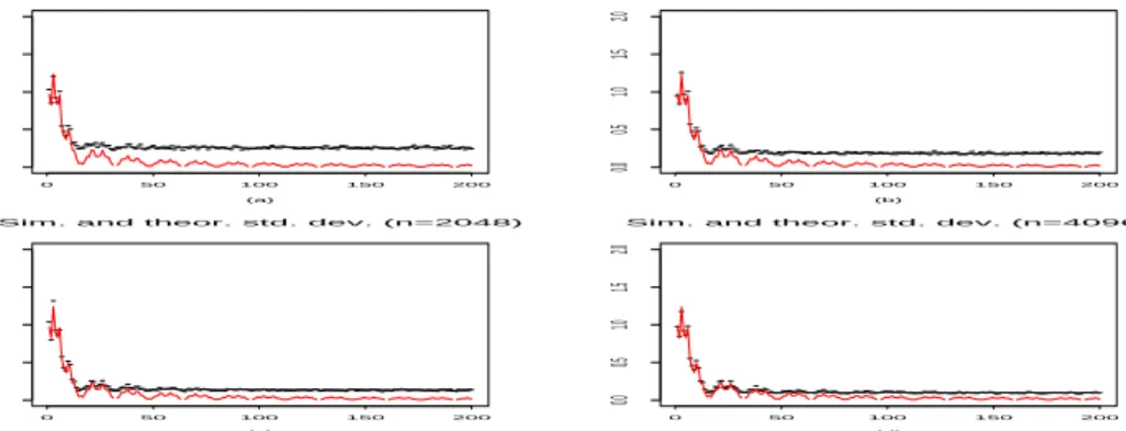
Figure 2a through d display results of a small simulation study where the simulated and true variance of the amplitude spectrum according to

(9) are compared for different sample sizes. At each frequency N =200

simulations are carried out and the amplitude spectrum was estimated. The

empirical standard deviations multiplied by √n are plotted in figures 2a

through d (black line) together with their asymptotic counterparts (red line). Convergence to the asymptotic standard deviation is apparently faster for frequencies where the amplitude spectrum is large. These are exactly that are used for estimating time shifts.

n 512 1024 2048 4096

true value 0.0625 0.0625 0.0625 0.0625

median 0.06012 0.06073 0.06322 0.06300

mean 0.05856 0.05838 0.06306 0.06262

std.dev. 0.03816 0.02275 0.00918 0.005528

Table 1: Summary statistics of lag estimates. For each sample size, 200 simulations were carried out.

Figure 3a shows the amplitude spectrum and the phase estimate for one simulated series. Frequencies where the estimated amplitude spectrum is

above four times its standard deviation are highlighted by black squares in figures 3a and b. The resulting estimated phase line in figure 3b is obtained by linear regression using these points only, taking into account jumps modulo

2π. The red lines indicate 99% confidence intervals for the regression slope.

The regression line in figure 3b, with slope around 0.39, is obviously very

similar to the true phase spectrum (figure 1f) with slope 0.30. For a more

systematic illustration of finite sample properties of ˆΔ, a small simulation

study was carried out, with sample sizes n = 512,1024,2048 and n = 4096.

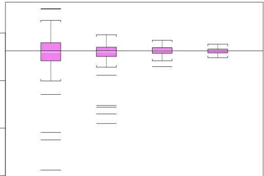
In each case we ran 200 simulations. Boxplots of ˆΔ (figure 4) based on 200

simulations (for each n) illustrate that estimation of Δ is very difficult for

n = 512. The accuracy of ˆΔ improves fast, however, with increasing sample

size. A detailed summary of this simulation study is given in table 1.

Finally, we examine in how far confidence intervals for Δ, based on

weighted linear regression of (j,φˆ) (with weights and residual variances

ob-tained from corollary 2) have the desired coverage probability. For each simulated series, the six frequencies with largest cross-spectral modulus were used in the regression, and 95%-confidence intervals were calculated using

es-timated variances of ˆφ at these frequencies. The coverage percentages, based

on 1000 simulations, turned out to be close the desired values, namely 93.9%,

93.5%, 94.8% and 94.8% for n = 512, 1024, 2048 and 4096 respectively.

5.2

El Ni˜

no and recruitment of new fish

Figures 5a and b display the components of the bivariate time series con-sisting of the Southern Oscillation Index (SOI) and recruitment (amount) of new fish in the central Pacific Ocean (figures 5a and b), ranging from

1950 to 1987 over a period of n = 453 months. The SOI relates changes

in air pressure to the temperature of the ocean at the surface. The data set can be found in Shumway and Stoffer (2000). Both time series exhibit cyclic components. The dominating periodic component in the SOI has a period of 12 months. The second series oscillates with a lower frequency, but a 12-months cycle is visible as well, at least in parts of the series. This is most obvious when looking at the amplitude of the estimated regression

cross spectrum in figure 5c which shows a dominating frequency at j = 38

indicating a period of 453/38≈12 months. In addition, a certain number of

moderate contributions are present at low frequencies. The slight influence of low frequency components is also visible directly in the SOI series, in that the mean and variability seem to be changing slowly. This feature is often

refered to in the literature as the El Ni˜no effect. We now proceed as in the simulated example. The estimated phase line in figure 5f is based on frequen-cies where the amplitude spectrum is large. The corresponding points are marked by black squares in figure 5e,f. Focussing on these points only, one can detect a linear structure. We may thus assume that there is a

frequency-independent shift Δ. Linear regression yields a slope estimate of about 0.1,

and thus ˆΔ = 0.1/(2π) ≈ 0.016 which corresponds to 453·0.1/(2π) ≈ 7.2

months. This indicates that the SOI signal leads the recruitment of new fish by about seven to eight months.

However, in view of figure 5c, better insight may be gained by separating high and low frequency components in the second series. We therefore carry out the analysis at separate levels of resolution. Figures 6a and b show trend

estimates ˆf₁ (SOI) and ˆf₂ (fish recruitment) obtained by wavelet

threshold-ing with s20-wavelets. The second trend function is decomposed further by separating the three coarsest resolution levels (figure 6c) from the fourth level (figure 6d). The fourth level represents the 12-month cycle, whereas the coarser parts (levels one to three, D4-S6) represent four to five year cy-cles that may be associated with corresponding cycy-cles in the warming of the Pacific Ocean. The estimated amplitude cross spectrum with significant fre-quencies marked by black squares are displayed in figure 6e and the resulting phase line with corresponding confidence intervals is presented in figure 6f. One notices again the distinct linear structure over this particular set of fre-quencies. The slope of this line is given by 0.17 indicating a lead of SOI of

453·0.17/(2π)≈ 12 months.

Because annual seasonality is the only common periodic oscillation be-tween SOI and the component D3 (figure 6g), time delays bebe-tween these two series are estimated in the time domain. The regression correlations between

the SOI trendf₁ and the component D3 is displayed in figure 6h. The annual

seasonality of the number of fish turns out to lag behind the SOI by about one month, indicating that an increased water temperature induces an increased

number of fish about one month later. This effect interferes with the El Ni˜no

effect which has periods of abnormal warming of the sea every four to five years. These results confirm similar findings on the interplay between water temperature and fish recruitment by a number of authors such as Murawski (1993), Victor et al. (2001), Shumway and Stoffer (2000), Rosen and Stoffer (2007), among others.

6

Final remarks

Analyzing multivariate dependence using the nonparametric regression spec-trum is particularily useful when the observed series have strong deterministic components. In this article we defined a simple estimator of the regression spectrum based on the periodogram. In contrast to the method in Beran and Heiler (2007) no trend estimation is required. Also, in contrast to the stationary case, no smoothing of the periodogram is needed. In addition, lag estimation in the time domain was considered in order to be able to deal with cases where dependence between two series occurs for a small number of frequencies only. The regression spectrum approach can be particular-ily powerful when used in combination with multiresolution analysis. Often, the strength, type and interpretation of dependencies differ at different levels. The SOI/fish recruitment data is a typical example of multilevel dependence. In future research, more formal methods should be developed for combining regression spectrum estimation and wavelet decomposition.

7

Acknowledgements

This research was supported in part by a grant of the German Research Foundation (DFG).

8

Appendix: Proofs

Proof 1 (of theorem 1) We have h_rs(j) =a_r(j)a_s(j), and

1 n2Ar(ωj)As(ωj)−hrs(j) =O(n −1_{). (16)} Then 1 nIrs(ωj)−hrs(j) = 1 n2[Br(ωj)As(ωj) +Ar(ωj)Bs(ωj)] +Op(n −1_{) +O(n}−1₎ =O_p(n−1/2).

For the second part consider

E(n−1I_rs(ω_j)) = 1

n2[Ar(ωj)As(ωj) +E(Br(ωj)Bs(ωj))],

=h_rs(j) +O(n−1)+n−1E(I_;rs(ω_j)).

Results from traditional spectral analysis show that E(I_;rs(ω_j)) converges to

2πh_;rs(ω_j) uniformly for all frequenciesω_j so that 2) follows.

Note furthermore that

1 √ n a_r(j)B_s(ω_j) +B_r(ω_j)a_s(j) =:α(j) +iβ(j), (17) where α(j) = √1 n cos(ω_jt)[a_r(j)_s(t) +a_s(j)_r(t)], (18) β(j) = √1 n sin(ω_jt)[a_r(j)_s(t)−a_s(j)_r(t)]. (19)

Consider now the variance of the adjusted periodogram (the result for covari-ances follows similarly):

var(n−1I_rs(ω_j)) =n−1E[|α(j) +iβ(j)|2] (20)

+cov(n−1I_;rs(ω_j), α(j) +iβ(j)) (21) +cov(α(j) +iβ(j), n−1I_;rs(ω_j)) (22)

+var(n−1I_;rs(ω_j)). (23)

Using standard results from Brockwell and Davis (p.429) yields

cov(I_;rs(ω_j), I_;rs(ω_j)) = ⎧ ⎨ ⎩ Σ_rrΣ_ss+O(n−1); 0< ω_j =ω_j < π, Σ_rrΣ_ss+ Σ_rsΣ_sr+O(n−1); ω_j =ω_j ∈ {0, π}, O(n−1); ω_j =ω_j,

where the remainders contain the fourth order cumulants between _r(i) and

_s(i). The covariances in (21) and (22) consist of terms of the form

cov(I_;rs(ω_j), B_r(ω_j)) = 1 n t,u,v exp(−iω_j(t−u+v))E(_r(t)_s(u)_r(v)) = E(r(1) 2 s(1)) n n t=1 exp(iω_jt) = 0,

where E(_r(t)2_s(t))is independent of t. Simple considerations show that the

2p-dimensional real valued random vector

U_n(ω_j) =n−1/2 (t) cos(ωjt)

(t) sin(ω_jt)

(24)

is asymptotically normal with mean 0 and covariance matrix

E(U_n(ω_j)U_n(ω_j)T) = 1 2 Σ 0 0 Σ .

Furthermore, for all Fourier frequencies ω_j =ω_j,

E(U_n(ω_j)U_n(ω_j)T) = 0. (25)

Therefore,

n−1E(B_r(ω_j)B_s(ω_j))

=n−1cov(_r(t)(cos(ω_jt)−isin(ω_jt)),_s(t)(cos(ω_jt)−isin(ω_jt)))

= 1

2(Σrs+ Σsr) = Σrs.

Similarly, for all pairs (r, s), 1≤r=s≤p,

var(n−1/2B_r(ω_j)) = Σ_rr and cov(B_r(ω_j), B_s(ω_j)) =cov(B_s(ω_j), B_r(ω_j)) = 0. Noting that n t=1 cos2(ω_jt) = n 2,

the variance in (20) follows from

τ_α2(j) :=var(α(j)) = 1 n n t=1 cos2(ω_jt)[Σ_rr|a_s(j)|2+ Σ_ss|a_r(j)|2 +a_s(j)a_r(j)cov(_r(t), _s(t)) +a_r(j)a_s(j)cov(_s(t), _r(t))] = 1 2(Σrr|as(j)| 2_{+ Σ} ss|ar(j)|2) + ΣrsRe{as(j)ar(j)}.

Similarily, τ_β2(j) :=var(β(j)) = 1 2(Σrr|as(j)| 2_{+ Σ} ss|ar(j)|2)−ΣrsRe{as(j)ar(j)} and τ_α,β(j) :=cov(α(j), β(j)) = 1 n n t=1

cos(ω_jt) sin(ω_jt)cov(a_s(j)_r(t) +a_r(j)_s(t), a_r(j)_s(t)−a_s(j)_r(t)),

where the covariance is independent of t. Using the orthogonality relations

for trigonometric functions we get that τ_α,β(j) = 0.

For the asymptotic distribution, write

√

n(1

nI(ωj)−hrs(j)) =α(j) +iβ(j) +Op(n −1/2_).

According to (24) the asymptotic distribution of the real and the imaginary

part are both univariate normal. Moreover, α(j) and β(j) are uncorrelated

and hence asymptotically independent. Hence,

α(j) β(j) d → N 0, τ_α2(j) 0 0 τ_β2(j) ,

andα(j)+iβ(j)converges in distribution to a complex valued normal random

variable with mean 0 and variance

τ_α2_+iβ(j) = τ_α2(j) +τ_β2(j) = Σ_rr|a_s(j)|2+ Σ_ss|a_r(j)|2. (26) This implies √ n(1 nIrs(ωj)−hrs(j)) d → Nc(0,Σrr|as(j)|2+ Σss|ar(j)|2). (27)

The result for finite samples (ω_j1, . . . , ω_jk) follows as usually by applying the

Cramer-Wold device.

Proof 2 (of theorem 2)

Lemma 2 Assume that the sequence {(i)}, i= 1, . . . , n, is of the form (i) = ∞ j=−∞ A(j)Z(i−j), (28)

where A(j) = (A_lk(j))_1≤l,k≤p arep×p-matrices such that for all pairs (l, k),

j∈Z

|A_lk(j)||j|12 _<∞_,

and the sequence Z(i) is independent and identically distributed with mean 0

and non-singular covariance matrix Σ.

Then, g(ω_j) =n−1/2 (t) cos(ωjt) (t) sin(ω_jt) = g₁(ω_j) g₂(ω_j)

with g_l(ω_j) = (g_l1(ω_j), . . . , g_lp(ω_j))T, l ∈ {1,2}, converges in distribution to

a 2p-dimensional random variable with mean 0 and asymptotic covariance

matrix π C(ω_j) Q(ω_j) −Q(ω_j) C(ω_j) ,

whereh(ω_j) = 1₂(C(ω_j)−iQ(ω_j))withC(ω_j) = [c_;rs(ω_j)]_1≤r,s≤pandQ(ω_j) =

[q_;rs(ω_j)]_1≤r,s≤p is the spectral density matrix of (i) at Fourier frequency

ω_j = 2πj/n. Furthermore g(ω_j) and g(ω_j) are asymptotically independent

for ω_j =ω_j.

We now turn to the proof of theorem 2. The first two parts of the proof are similar to those of theorem 1. For the asymptotic distribution and variance consider equations (20)-(23). Refer again to Brockwell and Davis (p. 431) to get cov(I_;rs(ω_j), I_;rs(ω_j)) = ⎧ ⎪ ⎪ ⎪ ⎪ ⎨ ⎪ ⎪ ⎪ ⎪ ⎩ (2π)2h_;rr(ω_j)h_;ss(ω_j) +O(n−1/2_); 0< ω_j =ω_j < π, (2π)2(h_;rr(ω_j)h_;ss(ω_j) +h_;rs(ω_j)h_;sr(ω_j)) +O(n−1/2); ω_j =ω_j ∈ {0, π}, O(n−1); ω_j =ω_j.

Using the results of lemma 2,

var(√1

nBr(ωj)) = 2πh;rr(ωj) (1≤r≤p), (29)

and use the notation

h_;rr(ω_j) =c_;rs(ω_j)−iq_;rs(ω_j). Then, cov(√1 nBr(ωj), 1 √ nBs(ωj)) =cov(g_1r(ω_j)−ig_2r(ω_j), g_1s(ω_j) +ig_2s(ω_j)) =c_;rs(ω_j) +iq_;rs(ω_j)−iq_;rs(ω_j)−c_;rs(ω_j) = 0. (30)

Due to lemma 2 and equations (29) and (30),

α(j) +iβ(j)→ Nd _c(0,(2π|a_s(j)|2h_;rr(ω_j) + 2π|a_r(j)|2h_;ss(ω_j))),

where α(j) +iβ(j) is defined in (17). The remaining parts (21) and (22)

consist of terms of the form

cov(I_;rs(ω_j), B_r(ω_j)) = t,u,v exp(−iω_j(t−u+v))E(_r(t)_s(u)_r(v)), with E(_r(t)_s(u)_r(v)) = p r1,r2,r3=1 E(Z_r1(1)Z_r2(1)Z_r3(1)) j A_r,r1(j)A_s,r2(j+u−t)A_r,r3(j+v−t),

whereA_rr1(j)is the(r, r₁)th entry of the matrixA(j)andE(Z_r1(t)Z_r2(t)Z_r3(t))

is the third order cumulant between the components Z_r1(t), Z_r2(t) andZ_r3(t)

of Z(t). Because (i) is of the form (28),

|cov(I_;rs(ω_j), B_r(ω_j))| ≤

t,u,v

|E(_r(t)_s(u)_r(v))|<∞,

Proof 3 (of Theorem 3)

1. Results of Brillinger (1996) prove wavelet thresholding estimators to

be consistent of order O_p(n−1/2_{). The regression cross covariance is a}

continuous function of θ, the vector of wavelet coefficient of f_r and f_s,

so that the estimator uˆmax_rs is a continuous function of θˆ. Consistency

of θˆthen implies consistency of umax

rs . 2. Due to (14) and (15),

γ_rs (ˆumax_rs ,θˆ) = 0 and γ_rs (umax_rs , θ₀) = 0.

Applying the mean value theorem gives

γ_rs (ˆumax_rs ,θˆ)−γ_rs(umax_rs ,θˆ) =γ_rs(˜u_rs,θˆ)(ˆumax_rs −umax_rs ),

where u˜ lies on a line connecting uˆmax_rs and umax_rs . Therefore,

ˆ umax_rs −umax_rs =−γ rs(umaxrs ,θˆ) γ_rs(˜u_rs,θˆ) . Furthermore, γ_rs (umax_rs ,θˆ) =γ_rs(umax_rs , θ₀) =0 + ∂ ∂θγ rs(umaxrs , θ) θ=˜θ _T ·(ˆθ−θ₀)

for suitably chosen θ˜, and

ˆ umax_rs −umax_rs =− 1 γ_rs(˜u_rs,θˆ) ∂ ∂θγ rs(umaxrs , θ) θ=˜θ _T (ˆθ−θ₀).

Due to consistency of θˆand uˆmax_rs ,

γ_rs(˜u_rs,θˆ) = γ_rs(umax_rs , θ₀) + (γ_rs(˜u_rs,θˆ)−γ_rs(umax_rs ,θˆ)) + (γ_rs(umax_rs ,θˆ)−γ_rs(umax_rs , θ₀)) =γ_rs(umax_rs , θ₀) +O_p(n−1/2), and ∂ ∂θγ rs(umaxrs , θ) θ=˜θ = ∂ ∂θγ rs(umaxrs , θ) θ=θ0 +O_p(n−1/2).

Then, ˆ umax_rs −umax_rs =− 1 γ_rs(umax rs , θ0) ∂ ∂θγ rs(umaxrs , θ0) T (ˆθ−θ₀)(1 +O_p(n−1/2)).

The central limit theorem for √n(ˆθ−θ₀)implies that √n(ˆumax

rs −umaxrs ) is asymptotically normal with mean 0 and covariance

var(ˆumax_rs ) = ∂ ∂θγrs (umaxrs , θ)_{θ=θ0 T} var(ˆθ) ∂ ∂θγrs (umaxrs , θ)_θ=θ0 γ_rs(umax rs , θ0)2 .

References

[1] Beran, J. and Ghosh, S. (2000). Estimation of the dominating frequency for stationary and nonstationary fractional autoregressive models. Jour-nal of Time Series AJour-nalysis, Vol. 21, No. 5, 517-533.

[2] Beran, J. and Heiler, M. (2007). A Nonparametric Regression Spectrum for Analyzing Multivariaten Time Series. Journal of Multivariate Analy-sis, in press.

[3] Brillinger, D. (1994). Uses of Cumulants in Wavelet Analysis. Proc. SPIE, Advanced Signal Processing, Vol. 2296, 2-18.

[4] Brillinger, D.R. (1996). Some Uses of Cumulants in Wavelet Analysis. Nonparametric Statistics, Vol. 6, 93-114.

[5] Brockwell, P.J, and Davis, R.A. (1987). Time Series: Theory and Meth-ods. Springer, New York.

[6] Daubechies, I. (1999). Ten Lectures on Wavelets. Society for Industrial and Applied Mathematics, Philadelphia.

[7] Donoho, D.L. and Johnstone, I.M. (1994). Ideal Spatial Adaption by Wavelet Shrinkage. Biometrika, Vol. 81, No.3.

[8] Donoho, D.L. and Johnstone, I.M. (1995). Adapting to Unknown Smooth-ness Via Wavelet Shrinkage. Journal of the American Statistical Associ-ation, Vol. 90.

[9] Grenander, U. and Rosenblatt, M. (1957). Statistical analysis of station-ary time series, Wiley, New York.

[10] Hannan, E.J. (1970). Multiple time series. Wiley, New York.

[11] Heiler, M. (2007). A Nonparametric Regression Spectrum: Estimation, Asymptotic Properties and Data Analysis. Dissertation, University of Konstanz, Konstanz, 2007.

[12] Johnstone, I.M. and Silverman, B.W. (1997). Wavelet Threshold Esti-mators for Data with Correlated Noise. Journal of the Royal Statistical Society, Series B, Vol. 59, No. 2, 319-351.

[13] Murawski, S.A. (1993). Climate change and marine fish distributions: forecasting from analogy. Transactions of the American Fisheries Society, Vol. 122, 647-658.

[14] Percival, D.P. and Walden, A.T. (2000). Wavelet methods for time series analysis. Cambridge University Press, Cambridge.

[15] Pollard, D. (1984). Convergence of Stochastic Processes. 2nd _Edition,

Springer, New York.

[16] Polya G. and Szeg¨o G. (1964). Aufgaben und Lehrs¨atze aus der Analysis,

Erster Band, 3. Auflage. Springer, Berlin.

[17] Priestley, M.B. (1989). Spectral Analysis and Time Series, 6th Edition,

Academic Press, London.

[18] Rosen, O. and Stoffer, D.S. (2007). Automatic estimation of multivariate spectra via smoothing splines. Biometrika, 94, No. 2, 335-345.

[19] Shumway, R.H. and Stoffer, D.S. (2000). Time series analysis and its

applications, 2nd _{Edition. Springer, New York.}

[20] Victor, B.C., Wellington, G.M., Robertson, D.R. and Ruttenberg, B.I.

(2001). The effect of the EL Ni˜no-Southern Oscillation event on the

dis-tribution of reef-associated labrid fishes in the eastern Pacific Ocean. Bulletin of Marine Science, Vol. 69, No. 1, 280-288.

simulated f1+eps1 (a) 0.0 0.2 0.4 0.6 0.8 1.0 −10 −5 0 5 10 simulated f2+eps2 (b) 0.0 0.2 0.4 0.6 0.8 1.0 −5 0 5 10 15 true f1 (c) 0.0 0.2 0.4 0.6 0.8 1.0 123 45 true f2 (d) 0.0 0.2 0.4 0.6 0.8 1.0 123 45 • • • • • • • •••• ••••••••••••••••••••••••••••••••••••••••••••••••••••••••••••••••••••••••••••••••••••••••

true spectral modulus

(e) 0 20 40 60 80 100 0.0 0.05 0.10 0.15 •• •• •• •• •• •• •• •• •• •• •• •• •• •• •• •• •• •• •• •• •• •• •• •• •• •• •• •• •• •• •• •• •• •• •• •• •• •• •• •• •• •• •• •• •• •• •• •• •• •

true phase spectrum

(f) 0 20 40 60 80 100 −2 −1 0 1 2 3 • • • •• • • • •• • ••• ••••••••••••••••••••••••••••••••••••••••••••••••••••••••_{••••••••••••••••••••••••••••••} modulus of cross−spectrum (g) 0 20 40 60 80 100 0.0 0.05 0.10 0.15 • •• • • •• • • •• • •• • • • • • • • • • • • •• • • • • • • • • • • • • • • • • •• • •• • • • • • • • • • • • • • • • • • • •• •• • • • • • • •• • • • • • • • • • • • • • • • • • •• • • •

estimated phase spectrum

(h) phase 0 20 40 60 80 100 −3 −2 −1 0123

Figure 1: Simulated series of length n = 2048 (figures 1a,b), as defined in

section 5.1, trend components (figures 1c,d), and amplitude and phase of the true regression spectrum (figures 1e,f). Estimates of the amplitude and phase spectrum based on the periodogram are given figures 1g and h.

• • • • • • • •• •• ••••••••••••••••••••••••••••••••••••••••••••••••••••••••••••••••••••••••••••••••••••••••••••••••••••••••••••••••••••••••••••••••••••••••••••••••••••••••••••••••••••••••••••••••••••••••••••• Sim. and theor. std. dev. (n=512)

(a) 0 50 100 150 200 0.0 0.5 1.0 1.5 2.0 • • • ••• • •• •• ••••••••••••••••••••••••••••••••••••••••••••••••••••••••••••••••••••••••••••••••••••••••••••••••••••••••••••••••••••••••••••••••••••••••••••••••••••••••••••••••••••••••••••••••••••••••••••• Sim. and theor. std. dev. (n=1024)

(b) 0 50 100 150 200 0.0 0.5 1.0 1.5 2.0 • • • ••• • •• •• •• ••••••••••••••••••••••••••••••••••••••••••••••••••••••••••••••••••••••••••••••••••••••••••••••••••••••••••••••••••••••••••••••••••••••••••••••••••••••••••••••••••••••••••••••••••••••••••• Sim. and theor. std. dev. (n=2048)

(c) 0 50 100 150 200 0.0 0.5 1.0 1.5 2.0 • • • ••• • •• • • •• ••••••••• •••••••••••••••••••••••••••••••••••••••••••••••••••••••••••••••••••••••••••••••••••••••••••••••••••••••••••••••••••••••••••••••••••••••••••••••••••••••••••••••••••••••••••••••••• Sim. and theor. std. dev. (n=4096)

(d) 0 50 100 150 200 0.0 0.5 1.0 1.5 2.0

Figure 2: Simulated and theoretical (red line) standard deviations for the

am-plitude spectrum for various sample sizes n = 512,1024,2048 and n= 4096.

For each sample size, 200 simulations were carried out at each individual frequency. • • • • • • • • • • • • • • •• •• ••• • •••••••••• •• • •••• • •• ••• ••• •• modulus of cross−spectrum (a) 0 10 20 30 40 50 0.0 0.05 0.10 0.15 • • • • • •• • • • • • •• • • • • • • • • • • • • • • • • • • • • • • • • • • • • • • • • •• • • estimated phase line with c.i.

(b) phase 0 10 20 30 40 50 −3 −2 −1 0123

Figure 3: Estimates of the amplitude and phase spectrum based on the

periodogram for frequencies j = 1, . . . ,50. Important common frequencies

are marked by black squares. The estimated phase line (solid line) is based on these frequencies. The red lines represent 99% confidence intervals.

−0.2

−0.1

0.0

0.1

n.512 n.1024 n.2048 n.4096

Figure 4: Boxplots of simulated lag estimates for n = 512,1024,2048 and

n = 4096. For each sample size, 200 simulations were carried out. The true