A PARADOX OF INCONSISTENT PARAMETRIC
AND CONSISTENT NONPARAMETRIC REGRESSION
By
Peter C. B. Phillips and Liangjun Su
June 2009
COWLES FOUNDATION DISCUSSION PAPER NO. 1704
COWLES FOUNDATION FOR RESEARCH IN ECONOMICS
YALE UNIVERSITY
Box 208281
New Haven, Connecticut 06520-8281
http://cowles.econ.yale.edu/
A Parodox of Inconsistent Parametric and Consistent
Nonparametric Regression
∗
Peter C. B. Phillips
Yale University, University of Auckland
University of York & Singapore Management University
Liangjun Su
School of Economics
Singapore Management University
May 31, 2009
Abstract
This paper explores a paradox discovered in recent work by Phillips and Su (2009). That paper gave an example in which nonparametric regression is consistent whereas parametric regression is inconsistent even when the true regression functional form is known and used in regression. This appears to be a paradox, as knowing the true functional form should not in general be detrimental in regression. In the present case, local regression methods turn out to have a distinct advantage because of endogeneity in the regressor. The paradox arises because additional correct information is not necessarily advantageous when information is incomplete. In the present case, endogeneity in the regressor introduces bias when the true functional form is known, but interestingly does not do so in local nonparametric regression. We examine this example in detail and propose two new consistent estimators for the parametric regression, which address the endogeneity in the regressor by means of spatial bounding and bias correction using nonparametric estimation. Some simulations are reported illustrating the paradox and the new procedures.
JEL classification: C13, C14.
Keywords: Bias-correction, Endogeneity, Kernel regression, L2 regression, Location shift,
Nonparametric IV, Nonstationarity, Paradox, Spatial regression, Structural estimation.
∗Phillips acknowledges partial support from NSF Grant #SES 06-47086. Address correspondence to Peter C.
B. Phillips, Cowles Foundation for Research in Economics, Yale University, Box 208281, New Haven, Connecticut USA 06520-8281; e-mail: [email protected]. Liangjun Su, School of Economics, Singapore Management University, 90 Stamford Road, Singapore 178903; e-mail: [email protected].
1
Introduction and Motivation
Recent work (Phillips and Su, 2009, hereafter PS) drew attention to an interesting example in which parametric regression is inconsistent when the true functional form is known and yet, surprisingly, nonparametric regression is consistent. This note explores that example and the resulting paradox in more detail and suggests modifications to parametric regression which remove the inconsistency.
The example given in PS involves cross section regression with some systematic location shifts in an endogenous regressor. The location shifts may be regarded as a form of instrumen-tal variable effect that influences observations of the regressors and assists in identifying the regression curve. In particular, in the linear regression model
yi =β0+β1Xi+ui, E(ui|Xi)6= 0, E(ui) = 0, (1.1) the endogenous regressorXi is assumed to satisfy
Xi=μα1{i∈Aα}+uxi, (1.2) and, by virtue of its moving intercept
μα = αLn
2m , α=−m,−m+ 1,· · ·, m, (1.3) Xiis subject to(2m+ 1)location shifts that are equally spaced over the interval(−Ln/2, Ln/2). Theuxiare random quantities that may have compact[u, u]or infinite (−∞,∞)support. The quantity Ln may be fixed or may increase slowly asn→ ∞(e.g., Ln= logn).The parameter m passes to infinity so that the distance(Ln
2m) between two contiguous location shifts shrinks to zero as m→ ∞. Data also accumulates at each location and we define
M = #{i∈Aα},
although it is not necessary thatM be fixed across different locations. The total observation count is thenn= (2m+ 1)M.As in PS, we requirem→ ∞butM can either befinite or pass to∞ and this dual possibility is denoted by writing(M, m)→ ∞.
Model (1.1) is a simple example of a structural equation with an endogenous regressor. The endogeneity is obviously a source of potential bias in regression, particularly in the absence of an observed instrumental variable. Curiously, not knowing the functional form of (1.1) and performing nonparametric kernel regressoin produces a consistent estimator in spite of the en-dogeneity, whereas conventional least squares regession which uses functional form information is inconsistent.
In addition to the linear model (1.1), PS also considered the nonlinear structural equation yi=g(Xi) +ui, E(ui|Xi)6= 0, E(ui) = 0, (1.4)
where the endogenous regressorXi is generated via (1.2) and (1.3). PS studied the local level (Nadaraya-Watson) kernel estimator ofg(x)
b g(x) = 1 n Pn i=1yiKh(Xi−x) 1 n Pn i=1Kh(Xi−x) , (1.5)
where K(·) is a kernel function, Kh(·) = h−1K(·/h) and h ≡ h(M, m) is a bandwidth pa-rameter. Let g0(x) and g00(x) denote the first and second derivatives of g(x), respectively. Let fu0x(·) denote the first derivative of the marginal probability density function (p.d.f.) of uxi,and f200(u, ux) the second order partial derivative with respect to ux of the p.d.f. f(·,·) of (ui, uxi). The central finding of PS is that the nonparametric estimator bg(x) is consistent for g(x) under some standard regularity conditions, as detailed in the following theorem.
Theorem 1.1 Under Assumptions A1-A6 of PS with mλ replaced by dm = 2m/Ln, or As-sumptions A1-A2, A3(i), A4, A5 and A7-A9 of PS with L replaced byLn, we have
p M dmh µ b g(x)−g(x)−h2μ2(K) ½ g0(x) Z u u fu0x(p)dp+1 2g 00(x) ¾¶ →dN ¡ 0, σ2ν2(K) ¢ , (1.6) where μ2(K) =R x2K(x)dx, ν2(K) = R K(x)2dx, andσ2 =E¡u2i¢.
If the distribution of uxi has infinite support, so that fux(p) vanishes at infinity, then
R∞
−∞fu0x(p)dp = 0 and the linear bias term disappears in (1.6). Despite endogeneity in the
regressor, the local level estimator is consistent and asymptotically normally distributed. The price for the presence of endogeneity in the regression is the potentially slower rate of conver-gence. The convergence rate of the local level estimator relies on M dm = 2M m/Ln ∼ n/Ln. So the convergence rate, in the case of increasing Ln, is slower than the usual
√
nh-rate of convergence for local level estimate with a stationary regressor, which is related to the fi nd-ings of Wang and Phillips (2009) for nonparametric structural cointegrating regression, where again nonparametric regression is consistent. As PS argue, the location shifts act in a manner analogous to the random wandering feature of unit root regressors in a cointegrating regression equation and add variation to the regressor, and thereby explaining the consistency of simple nonparametric regression in both cases. Nevertheless, if the support of the distribution of uxi is compact, as is conventionally assumed in the nonparametric IV literature (e.g., Hall and Horowitz, 2005), the locational rangeLncan be a largefixed constant, and in this event simple local level regression is consistent and the usual √nh nonparametric rate of convergence is attained. This outcome contrasts with the attainable convergence rates for nonparametric IV estimation, which can be slow.
Applying the above result to the linear regression (1.1), we see that the nonparametric local level estimate bg(x) of g(x) = β0+β1x is consistent. Alternatively, if the functional form of
the regression is known, ordinary least squares regression can be applied to (1.1), giving b β1 = n X i=1 ¡ Xi−X¢yi/ n X i=1 ¡ Xi−X¢2, bβ0 =y−Xβb1,
where X = n−1Pni=1Xi, and y =n−1Pni=1yi. The parametric estimate of g(x) =β0+β1x is then given by bgp(x) = βb0 +bβ1x. Somewhat surprisingly, as remarked by PS, (bβ0,βb1) is inconsistent for(β0, β1)whenLnisfixed and, correspondingly,bgp(x)is inconsistent forg(x)at all points exceptx=E(uxi).WhenLn→ ∞asn→ ∞,consistency of the parametric estimate can be achieved but at the cost of the presence of a substantial bias term which seems difficult to eliminate. This outcome is paradoxical, as local level regression is consistent whereas linear parametric regression that uses the true functional form and global information is inconsistent. Clearly, using all information is costly here. The reason, of course, is the endogeneity in the regressor (1.1). Intriguingly, however, partial information usage of the type employed in kernel regression avoids most of the problems associated with parametric regression.
To illustrate the phenomenon, we generate a sample of n = 500 observations from the following system yi = β0+β1Xi+ui, β0= 10, β1 =−1, Xi = μα1{i∈Aα}+uxi, ui = 2 ( yi+γuxi)/ ¡ 1 +γ2¢1/2,
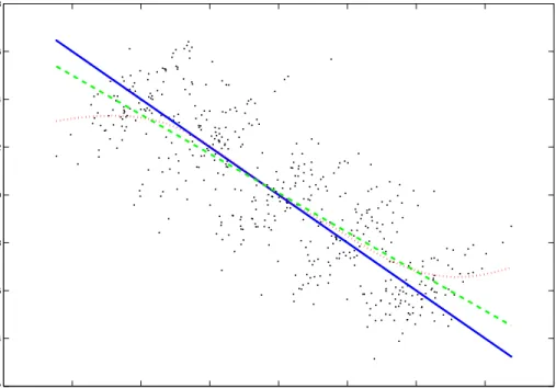
whereγ= 2.07,( yi, uxi)areiid N(0, I2),andμα ∈{−4,−2,0,2,4}.Using the above notation, this corresponds to the case where m = 2,and Ln = 8.When γ= 2.07,the error correlation coefficient is corr(ui, uxi) = 0.9, implying strong endogeneity in the structural equation. Fig 1 provides a typical sample plot of data generated from this system. Also displayed are the true linear regression line, the local level nonparametric estimate (using a Gaussian kernel and Silverman’s rule of thumb for the bandwidth choice) and thefitted OLS estimate obtained for these data. Clearly, the local level estimate considerably outperforms the parametric estimate of the regression line over a wide range of the support of the regressor. But at the tails of the support the endogeneity bias becomes manifest and the location shifts lose power in identifying the regression line. Since it uses local information and does so increasingly as the sample size rises, the local level estimator at interior points of the domain of the regressor very effectively attenuates distortion from tail observations. On the other hand, parametric linear regression, which treats all observations as equally important and applies global information infitting the regression line, is inevitably subject to potential distortions from tail observations.
This example makes clear that local nonparametric regression has more robustness advan-tages beyond robustness to specific functional form, for which it is commonly celebrated. As shown here, nonparametric regression may also display a robustness to endogeneity in a re-gression by concentrating attention on local information and attenuating tail information that may be more heavily subjected to endogeneity effects.
−8 −6 −4 −2 0 2 4 6 8 2 4 6 8 10 12 14 16 18 X i yi
Figure 1: Local level nonparametric (dotted) and linear regression (dashed) estimates of the true regression line (solid) using the full sample (scatter plot) over all locations.
Intuitively, any regression approach like conventional parametric regression that uses global information can be subject to distortionary effects from outlying observations. Such behavior is very well known in statistics. Anscombe (1960) coined the term ‘outlier’, provided a brief history of the subject, and suggested trimming techniques to attentuate the effects of outliers in regression based on the insurance analogy of ‘protection and premium’ to guard against unwanted effects. In the present context, the reason for the outlier effect is that at the limits of the domain of definition, the observations are more affected by the endogeneity of Xi, so bias arising from the ends of the domain can dominate a global regression and result in inconsistency. By contrast, in nonparametric regression mainly local information is used in estimation so the endogeneity effects of Xi in the tail can be well controlled and first order bias, at least, can be eliminated in local regression. In effect, by concentrating attention on the cluster of observations around each point, nonparametric regression localizes attention and removes outlier effects. This heuristic suggests that to recover the true regression line by a parametric method, a natural approach is to modify the regression by removing the effects of tail observations. The idea is comparable to that of trimming or Winsorizing the data, on which there is a large literature in statistics stemming largely from Anscombe’s (1960) study (e.g. Welsh, 1987; Chen, Welsh and Chan, 2001). In the present context, to use Anscombe’s analogy, the idea is to provide protection (against the possible effects of endogeneity) by paying a premium in terms of losing some observations. Kernel regression accomplishes this task by using data that is effectively in the locality of each individual regression point, thereby sacrificing an (asymptotically larger) infinity of observations to achieve a local regression fit and, incidentally in the process, protection from the effects of endogeneity.
The remainder of the paper is organized as follows. Section 2 studies the asymptotic properties of the OLS estimator (βb0,bβ1),demonstrates its inconsistency for the fixedLn case, and derives the asymptotic distribution of (βb0,bβ1). Section 3 proposes two new consistent estimators of (β0, β1) when Ln is either fixed or increasing slowly as n → ∞. The first is a spatialL2estimator which is obtained by regressing the nonparametric local level estimatebg(x)
on (1, x), using a continuous number of pseudo-observations on(x,bg(x)) wherex is spatially restricted to be bounded away from the two tails. The second is a bias-corrected OLS estimator of(β0, β1)that is based on the spatialL2 regression residuals. For both cases, we show that the
resulting estimators are consistent and asymptotically normally distributed. The consistency rate is parametric in the case where Ln =L is fixed, and
p
n/Ln in the case where Ln → ∞ asn→ ∞.Section 4 reports some simulation evidence and Section 5 concludes. Proofs of the main results are given in Section 6.
2
Limit Theory for Parametric Regression
To study the asymptotic properties of the OLS estimator (βb0,βb1), we make the following assumptions.
Assumption 1.
(i) (ui, uxi), i= 1,· · · , n,are independent and identically distributed (iid). (ii) E(ui) = 0, and E(u2i) =σ2.
(iii) E(uxi) =μx,and Var(uxi) =σ2x.
The above assumption is fairly standard in cross-sectional regression, although we do not make allowance for unconditional heterogeneity in (ui, uxi). Note that it is not assumed that the mean of uxi is zero, and conditional homoskedasticity is not assumed for the error term ui in the structural equation.
2.1
Inconsistency of
(
b
β
0,
β
b
1)
Under Assumption 1, wefirst derive the probability limit of the OLS estimatorbβ1and show that it is inconsistent forβ1 whenLnisfixed. The probability limit ofβb0 follows straightforwardly.
Write b β1=β1+n −1Pn i=1 ¡ Xi−X ¢ ui n−1Pn i=1 ¡ Xi−X ¢2 . (2.1)
First, by the definition of {μα}and the WLLN, we have 1 n n X i=1 ¡ Xi−X ¢2 = 1 2m+ 1 m X α=−m 1 M X i∈Aα ∙ Lnα 2m + (uxi−ux) ¸2 = L 2 n 4m2(2m+ 1) m X α=−m α2+ 1 n n X i=1 (uxi−ux)2+ Ln m(2m+ 1) m X α=−m α M X i∈Aα (uxi−ux) = L 2 n 2m2(2m+ 1) m X α=1 α2+σ2x+oP (1) = L 2 n 12 {1 +o(1)}+σ 2 x+oP(1), (2.2)
whereux=n−1Pni=1uxi,and the third line follows from the WLLN and Chebyshev inequality providedM m/L2 n → ∞asn→ ∞.1 1Letting T n ≡ m(2Lmn+1)Smα=−mMα Si∈Aα(uxi−μx) = Ln m(2m+1) Sm α=−m α M S i∈Aα(uxi−ux), then E(Tn) = 0,and Var(Tn) = L2 n M m2(2m+1)2 Sm α=−mα 2σ2 x=O L2 n M m =o(1).
Next 1 n n X i=1 ¡ Xi−X ¢ ui = 1 2m+ 1 m X α=−m 1 M X i∈Aα µ Lnα 2m +uxi−ux ¶ ui = Ln 2m(2m+ 1) m X α=−m 1 M X i∈Aα αui+ 1 n n X i=1 uxiui− ux n n X i=1 ui = Ln 2m(2m+ 1) m X α=−m 1 M X i∈Aα αui+E(uxiui) +oP(1).
Consider thefirst term in the last expression. LetT1n= 2m(2Lmn+1)Pmα=−mM1
P i∈Aααui.Then E(T1n) = 0 asE(ui) = 0,and Var(T1n) = L2n 4m2(2m+ 1)2Var à m X α=−m 1 M X i∈Aα αui ! = L 2 nσ2 4M m2(2m+ 1)2 m X α=−m α2 =O µ L2n M m ¶ =o(1). Hence T1n=oP(1)and 1 n n X i=1 ¡ Xi−X¢ui =E(uxiui) +oP (1). (2.3)
Combining (2.1), (2.2) and(2.3) yields
b β1=β1+ E(uxiui) +oP (1) L2 n 12 {1 +o(1)}+σ2x+oP (1) =β1+E(uxiui) L2 n 12 +σ2x {1 +oP (1)}, (2.4) thereby giving the following result.
Lemma 2.1 Suppose Assumption 1 holds and M m/L2n → ∞. Then
b
β1=β1+EL2(uxiui)
n 12 +σ2x
{1 +oP(1)}.
The following remarks explore the implications of the above lemma, considering the two cases whereLn=Lis fixed andLn→ ∞ asn→ ∞.
Remark 1. In the first case (Ln=L fixed),βb1 has the probability limit plimn→∞βb1 =β1+E(uxiui)
L2
12 +σ2x ,
and is inconsistent unlessE(uxiui) = 0,viz.,Xi is exogenous. Forbβ0,we have b β0−β0 = −X³βb1−β1´+n−1 n X i=1 ui (2.5) →p −μx E(uxiui) L2 12 +σ2x .
so βb0 is inconsistent for β0 unless either μx = 0 or E(uxiui) = 0. Hence, the parametric estimator bgp(x) = bβ0+βb1x is inconsistent for g(x) =β0 +β1x at all points except x = μx. By contrast, according to Theorem 1.1, the nonparametric estimator is consistent for all x satisfying certain domain restrictions.
Remark 2. In the second case (Ln→ ∞), the OLS estimator bβ1 is consistent for β1 as
b
β1=β1+12E(uxiui) L2
n
{1 +oP (1)}→pβ1,
due to the strengthening signal in the regressor asLn→ ∞. This result, together with (2.5), implies that βb0 is consistent for β0, and so the parametric regression estimator of g(x) = β0 +β1x is also consistent However, if Ln diverges to infinity slowly like Ln = logn, the estimation bias may disappear at a very slow rate. For inferential purposes, we now derive the limit distribution of (βb0,bβ1).
2.2
Limit distribution
Tofind the limit distribution of (βb0,bβ1),we add the following assumption. Assumption 2. E[|ui|2+δ]<∞ and E[|uiuxi|2+δ]<∞ for some δ >0.
Letθ= (β0, β1)0andbθ= (βb0,bβ1)0.LetXi = (1, Xi)0,X= (X1,· · ·,Xn)0,u= (u1,· · · , un)0,
and y= (y1,· · ·, yn)0.Define Dn=diag(1, Ln), Γ= lim n→∞ ⎛ ⎝ 1 μx Ln μx Ln 1 12+ E(u2 xi) L2 n ⎞ ⎠, and Ω= lim n→∞ ⎛ ⎝ σ2 E(uxiu2i) Ln E(uxiu2i) Ln σ2 12+ Var(uxiui) L2 n ⎞ ⎠.
After centering, the limiting distribution of bθ is given in the following theorem. Theorem 2.2 Suppose Assumptions 1-2 hold and M m/L2n → ∞. Then
√ nDn ³ bθ−θ−¡X0X¢−1E¡X0u¢´→d N ¡ 0,Γ−1ΩΓ0−1¢. (2.6) Remark 3. Straightforward calculations show that
¡ X0X¢−1E(Xu) = E(uxiui) n−1Pn i=1 ¡ Xi−X¢2 Ã −X 1 ! ,
and Γ−1ΩΓ0−1 = lim n→∞c −2 n à ω11n ω12n ω12n ω22n ! , wherecn= 121 + σ 2 x L2 n, ω11n = σ2 144+ 2E¡u2x1¢σ2+μ2xσ2−2μxE¡ux1u21 ¢ 12L2 n + £ E¡u2 x1 ¢¤2 σ2+μ2 xVar(ux1u1)−2μxE ¡ u2 x1 ¢ E¡ux1u21 ¢ L4 n , ω12n = σ2 12 − μxσ2 12 + Var(ux1u1)−2μxE ¡ ux1u21 ¢ L2 n − E¡u2x1¢μxσ2 L3 n , and ω22n = σ2 12 + Var(ux1u1) +μ2xσ2−2μxE ¡ ux1u21 ¢ L2 n = σ 2 12 + Var((ux1−μx)u1) L2 n . An immediate implication of Theorem 2.2 is therefore that
√ n à b β0−β0+ X E(ux1u1) n−1Pn i=1 ¡ Xi−X ¢2 ! →d N ³ 0, lim n→∞c −2 n ω11n ´ , (2.7) Ln√n à b β1−β1− E(ux1u1) n−1Pn i=1 ¡ Xi−X ¢2 ! →d N ³ 0, lim n→∞c −2 n ω22n ´ , (2.8) IfLn→ ∞asn→ ∞,then the above calculation simplifies and
Γ−1ΩΓ0−1 = Ã 1 0 0 121 !−1Ã σ2 0 0 σ122 ! Ã 1 0 0 121 !−1 =σ2 Ã 1 0 0 12 ! .
In this case, the intercept estimator, after centering, is asymptotically independent of the slope estimator, and the the slope coefficient estimator has a faster convergence rate, due to the stronger signal in the regressor. In contrast, in the fixed Ln case, the two estimators are asymptotically dependent, have the same rate of convergence, and the range of location shifts contributes to the asymptotic variance formula in (2.6) in a complicated way.
Remark 4. In spite of the O(√n) convergence rate for the intercept estimator and the O(Ln√n) convergence rate for the slope estimator, the result in (2.6) does not seem useful for inferential purposes because the bias term in (2.6) does not appear to be estimable at the required √n/L2n-rate (for the intercept parameter) or√n/Ln-rate (for the slope parameter) to be eliminated (recall from (2.2) thatn−1Pni=1¡Xi−X
¢2
=OP
¡
L2n¢). It is worth mentioning that the residuals{uib}from the OLS regression are useless in constructing a consistent estimate ofE(Xiui)because of the orthogonality ofubiandXi.One may consider consistent estimation of E(Xiui)by estimating the modelfirst via the local level (or local linear) nonparametric method at interior points and then obtaining the nonparametric residuals from the structural equation. Unfortunately, this approach usually requires uniform consistency of the local level (or local
linear) estimate over the whole support of the regressor, which seems extremely difficult here given the fact that the variance of the regressor is expanding as the sample size increases or that the nonparametric estimates are only consistent at points within a subset of the interior of the support of the regressor for the fixedLncase.
Instead, the next section proposes two alternative methods to achievepn/Ln-consistent es-timation of(β0, β1)by direct use of the nonparametric level estimate in a parametric regression.
3
Spatial
L
2and Bias-Corrrected OLS Estimation
In this section we propose two methods for consistent estimation of(β0, β1).Thefirst method is a spatial L2 regression and the second method involves bias-corrected OLS estimation. The
L2 method treats the linear regression function as unknown, estimates it nonparametrically by
b
g(x), and then regresses bg(x) on (1, x) to estimate the unknown parameter (β0, β1) by mini-mizing a spatial L2 criterion function, using a continuum of pseudo-observations on(x,bg(x))
where x is restricted to be bounded away from the two tails. We prove that the resulting L2
estimator ispn/Ln-consistent, where Ln can be either fixed or pass to infinity as n→ ∞. In either case, we show that the OLS bias terms are corrected by using the residuals from theL2
regression, and the bias-corrected OLS estimators can only attain an O(pn/Ln) consistency rate, which is inherited from that of the L2 estimates.
3.1
Spatial
L
2regression
Noting that the local level estimatebg(x)is consistent forg(x) =β0+β1xin the interior of the regressor support, we propose to estimate the unknown parameterθ≡(β0, β1)0 by minimizing the following (spatial) L2 criterion
Sn(β0, β1) =
Z b a
(bg(x)−β0−β1x)2fb(x)dx (3.1) whereaand b arefinite integration limits that serve to truncate observations in the two tails,
b
f(x) =N−1Pn
i=1Kh(x−Xi) is a pseudo-estimate of the “density” ofXi,andN = 2mM/Ln signifies the effective number of observations used in the nonparametric estimation, which does not need to be observed in practice for implementation. Note that fb(x) is a weight function that serves to avoid division by zero and to perform trimming in areas of sparse support, and [a, b] defines a compact set on which the nonparametric estimates bg(x) are used in the estimation of (β0, β1). Clearly, (3.1) provides a trimming operation implicitly via the local nature of the estimatebg(x) and explicitly via the use of the (truncated) domain[a, b].
The minimizer of (3.1) eθ≡(βe0,eβ1)0 is given by e θ= Ã Rb afb(x)dx Rb axfb(x)dx Rb axfb(x)dx Rb a x 2fb(x)dx !−1Ã Rb abg(x)fb(x)dx Rb a xbg(x)fb(x)dx ! .
To develop the limit theory, we make the following assumptions.
Assumption 3. The probability density function (p.d.f.) f(·,·) of (ui, uxi) exists. f(·,·) has second order partial derivative f200(u, ux) with respect to ux such that f200(u, ux) is continuous in ux and
R R
|uf200(u, ux)|dudux < ∞. The marginal p.d.f. of uxi, fux(·), has second order
continuous derivatives such that R−∞∞ ¯¯fu0x(p)¯¯dp <∞,and R−∞∞ ¯¯fu00x(p)¯¯dp <∞. Assumption 4. Either one of the following conditions holds:
(i) The error term uxi has infinite support such that there exists a majorizing function Cf(·)and a diverging sequence cn=cn(Ln)such that |
R−Ln −∞ f(u, ux)dux+ R∞ Lnf(u, ux)dux|≤ c−n1Cf(u) with c−n1=O ¡ h2¢and R−∞∞ |u|Cf(u)du <∞. Ln→ ∞ as n→ ∞, and fux(Ln) = O(h2) as Ln→ ∞;
(ii) The error term uxi has compact support, i.e., uxi ∈[u, u] a.s. for somefinite numbers u and u. Ln is either fixed or tends to ∞ as n→ ∞.If Ln=L isfixed, Lis sufficiently large that x∈(−L/2 +u, L/2 +u)for all x∈[a, b].
Assumption 5. The kernel function K(x) is a uniformly bounded, symmetric p.d.f. such that R x4K(x)dx <∞.
Assumption 6. As (M, m) → ∞, M m/L2n → ∞, M mh4/Ln → 0, M m−3L3n → 0, and N−δ/2Ln→0.
Assumptions 3-4 are comparable to Assumptions A3 and A7-A9 in PS. Assumption 5 is standard and the symmetry assumption greatly simplifies derivations. Note that we impose undersmoothing (M mh4/Ln → 0) on the bandwidth in Assumption 6. The last requirement in Assumption 6 is needed to verify the Liapounov condition.
Theorem 3.1 Suppose Assumptions 1-6 hold. Then
√ N(eθ−θ)→d N ¡ 0, σ2Q−1¢, (3.2) where Q= Ã b−a b2−2a2 b2−a2 2 b3−a3 3 ! .
Remark 5. Despite the nonparametric convergence rate of the regressand bg(x), Theorem 3.1 indicates that the L2 estimate eθ is
√
N-consistent. It achieves the parametric √n-rate of consistency for the case offixedLn and its rate is only slightly worse than the parametric rate in the case whereLn is an increasing slowly varying function at infinity. In addition,eθ is not subject to any non-negligible asymptotic bias term. To obtain these results in Theorem 3.1, we
have applied two tricks implicitly. First, undersmoothing is required to eliminate the O¡h2¢ bias terms from thefirst stage nonparametric regression estimate ofg(x).This is standard in the nonparametric or semiparametric literature when the first stage nonparametric estimates are used in a second stage parametric or nonparametric estimation. Second, to reduce the variation of the nonparametric estimates, we have used integration in the L2 regression. The
smoothing operation of integration helps to produce the (nearly) parametric convergence rate ofeθ despite the slow nonparametric convergence rate ofbg(x).The mechanism is analogous to that of average marginal effect or derivative estimation.
Remark 6. Even though the structural error terms may be conditionally heteroskedastic, the asymptotic variance of eθ only depends on the unconditional variance σ2. For inferential
purposes, we need to choose(a, b)in theL2regression and estimateσ2. Letuie =yi−eβ0−βe1Xi.
We can estimateσ2 by eσ2 = 1nPin=1ue2i.It is straightforward to show thateσ2 is consistent for σ2. With this estimate, in principle one can obtain a consistent estimate of the asymptotic covariance matrix of√N(eθ−θ)usingσe2Q−1.But sinceN is not observed, this last estimate is not directly applicable in statistical inference. One approach is to replaceQ by its consistent estimate Qn= Ã Rb afb(x)dx Rb axfb(x)dx Rb axfb(x)dx Rb ax 2fb(x)dx !
because the quantity N that appears in the definition of fb(x) = N−1Pn
i=1Kh(x−Xi) and also in the scaling of the estimate,√N(eθ−θ),will cancel in inference. More explicitly, consider testing the null hypothsisH0 :Rθ=r,whereRis a full rankk×2matrix andrisk×1vector.
UsingQn we can construct the following Wald statistic as usual Wn=σe−2(Reθ−r)0(N Qn) (Reθ−r), and without knowledge ofN.
Remark 7. For the integration limits, we recommend choosing a = FX−1(λ) and b = FX−1(1−λ)whereFX−1(λ)denotes the sampleλ-th quantile of{Xi}andλ∈(0,0.5),although there is no reason for symmetric truncations in the two tails. Since in the extreme tails the nonparametric estimates bg(x) are highly distorted, so we recommend λ≥0.05 depending on the number of observationsn.The largerλ,the greater the proportion of observations that are trimmed and the greater the efficiency loss that results. We therefore do not want to trim too many observations and recommend λ≤0.30.In the simulations below, we study the effect of the truncation parameter (λ) on the L2 and bias-corrected OLS estimators. We find that for
sample sizesn= 500∼2000,the choiceλ= 0.15 works fairly well. It is worth mentioning that in the above theory, we only establish the asymptotic result forfixed(a, b).We conjecture the theory also works when one allows the integration range to expand slowly as n → ∞, under suitable controls on the rate of expansion.
3.2
Bias-corrected OLS estimation
We now propose a bias-correction procedure for the OLS estimator ofθ= (β0, β1)0 in the linear structural equation (1.1). Let ec=n−1Pni=1uiXi.e We define bias-corrected OLS estimators of β0 andβ1,respectively, as b β0c=bβ0+ X ec n−1Pn i=1 ¡ Xi−X ¢2 and βb1c=bβ1− e c n−1Pn i=1 ¡ Xi−X ¢2.
Due to the pn/Ln-rate of convergence of eθ = (eβ0,βe1)0, the L2 residuals eui only converge
to the true structural errors ui at a
p
n/Ln-rate (viz. eui −ui = OP(
p
Ln/n)). As a result, n−1Pni=1euiXi−E(uiuxi) =OP(pL5
n/n) due to the fact thatn−1
Pn
i=1Xi2 =OP(L2n),which is not theoP(Ln/√n) rate required for the complete removal of the bias of the OLS estimator
b
θ = (bβ0,βb1)0 in (2.7) and (2.8). This indicates that bθc ≡ (βb
0c,βb1c)0 does not have the same standardization and asymptotic variance asbθ.
Nevertheless, after re-scaling, we can show that bθc is
p
n/Ln-consistent for θ and it is asymptotically normally distributed with variance that can be easily estimated. The following theorem establishes the consistency and asymptotic normality ofbθc.
Theorem 3.2 Suppose Assumptions 1-3, and 5-6 hold. (i) If Assumption 4(i) holds or 4(ii) holds with Ln → ∞ as n→ ∞, then√N(bθc−θ)→d N(0,Ψ), where
Ψ=σ2q22
Ã
μ2x −μx
−μx 1
!
and q22 is the (2,2)element of Q−1.
(ii) If Assumption 4(ii) holds withLn=L fixed, then √N(bθc−θ)→d N(0,Ψ),where
Ψ=B−1ΥB−1, Υ=σ2 Ã L−1 L−1 L−1 c0Q−1c ! , B= Ã 1 μx μx L122 +E(u2 xi) ! , and c= (μx, cx)0 with cx = L 2 12 +E(u 2 xi).
Remark 8. Despite its potential slower convergence than the OLS estimatorbθ,Theorem 3.2 indicates that the estimator bθc is pn/Ln-consistent for θ. For inferential purposes we need to estimate the asymptotic covariance matrixΨ.Since Ln is not observed in practice and the researcher may not know whetherLnisfixed or tends to∞asn→ ∞,we propose an estimator of Ψthat is consistent under either scenario. In the Appendix, we show that
√ N³bθc−θ´=√N Bn−1n−1 n X i=1 Ã ui ¡ Xi, Xi2¢(eθ−θ) ! =Bn−1Rn
whereBn=n−1X0X, Rn=√N n−1 n X i=1 Ã ui ¡ Xi, Xi2¢(eθ−θ) ! = Ã √ N n−1Pn i=1ui b c0√N(eθ−θ) ! , and bc = n−1Pni=1¡Xi, Xi2 ¢0. Let b
uic = yi −bβ0c −βb1cXi. Theorems 3.1-3.2 suggest that we can consistently estimate the asymptotic variance of √N n−1Pn
i=1ui and
√
N(eθ−θ) by N n−2Pni=1bu2ic and n−1Pin=1ub2icbc0Q−n1bc, respectively.2 To estimate the asymptotic covariance between √N n−1Pni=1ui and bc0
√
N(eθ −θ), we need to use the Bahadur representation of
√
N(eθ−θ) given in the Appendix:
√ N(eθ−θ) = n X i=1 Ã ξi1 ξi2 ! +oP(1),
whereξi1 and ξi2 are defined in (6.11)-(6.12). Due to the automatic correction of endogeneity bias in nonparametric estimation and the use of undersmoothing, centering in the definition of ξi1 and ξi2 is not necessary. This representation motivates us to estimate the asymptotic covariance between√N n−1Pni=1ui andbc0√N(eθ−θ) by
b Υn,12=n−1 n X i=1 b uicbc0(bξi1,bξi2)0, wherebξi1 =q11RabKixubicdx+q12 Rb axKixbuicdx,bξi2=q21 Rb aKixubicdx+q 22Rb axKixbuicdx, Kix= Kh(Xi −x), and qst is the (s, t) element of Q−1. Plugging these expressions forbξi1 and bξi2 directly into Υbn,12 yields the simplification
b Υn,12=n−1 n X i=1 b u2icbc0Q−1 µZ b a Kixdx, Z b a xKixdx ¶0 .
Again, for the same reason as that used to obtain the asympotic variance of √N(eθ−θ) in Remark 6, we need to replace Q by Qn in practice. It follows that we can estimate the asymptotic variance-covariance matrix Ψby
b Ψn=Bn−1ΥbncBn−1 where b Υnc = Ã N n−2Pn i=1ub2ic Υbnc,12 b Υnc,12 n−1Pni=1ub2icbc0Q−n1bc ! . and Υbnc,12 = n−1Pni=1bu2icbc0Q−n1 ³Rb aKixdx, Rb axKixdx ´0
. It is straightforward to show that
b
Ψn →p Ψ, and statistical inference can be conducted as usual without observing N.Thus we have the following corollary.
2Here we useQ
Corollary 3.3 Under the conditions of Theorem 3.2, Ψbn→p Ψ.
Remark 9. Even though we only focus on the linear structural equation model as specified in (1.1), it is straightforward to extend our theory to the general nonlinear structural equation model. For simplicity and in order to apply the result of PS directly, we focus on the case of one endogenous regressor. Suppose{yi}is generated according to
yi=g(Xi, θ) +ui, E(ui|Xi)6= 0, (3.3) whereg(·, θ)is known up to thefinite dimensional parameterθ,and the endogenous regressor Xi satisfies (1.2) and (1.3). It is straightforward to show that the nonlinear least squares (NLS) estimatorbθof θ is inconsistent. As before, the nonparametric local level estimate bg(x) of g(x) = g(x, θ) is still consistent for a large portion of the domain of the regressor. Then, the unknown parameterθ can be estimated by minimizing the following (spatial)L2 criterion
Sn(θ) =
Z b a
(bg(x)−g(x, θ))2fb(x)dx, (3.4)
just as before. Let eθ denote the solution to the above minimization problem. Following the proof of Theorem 3.1, we can show that eθ is pn/Ln-consistent for θ under some regularity conditions. In addition, it can be established in an analogous way to that of Theorem 3.2 that the NLS estimator, after bias correction, is alsopn/Ln-consistent for θ. The details are straightforward and are thus omitted.
4
Simulations
This section reports a small set Monte Carlo experiment to evaluate the finite sample per-formance of the L2 and bias-corrected OLS estimators. Data is generated according to the
following data generating process (DGP):
yi = β0+β1Xi+ui, β0 = 10, β1=−1, Xi = μα1{i∈Aα}+uxi, μα = αLn 2m , α=−m,−m+ 1,· · ·, m, ui = σ( yi+γ(uxi−10))/ ¡ 1 +γ2¢1/2, σ=SX,
where yi are iid N(0,1), uxi are iid N(10,1) and independent of yi, and SX is the sample standard deviation of Xi. By construction, the signal to noise ratio is maintained at unity throughout the simulations in order to enhance comparability across experiments. Simulations are performed for γ= 0.32 (weak endogeneity, corr(ui, uxi)= 0.3) andγ = 2.07 (strong endo-geneity, corr(ui, uxi)= 0.9), and for the sample sizes n = 500, 1000, and 2000. We generate the location shift points μα as 2m + 1 evenly spaced points between [−logn,logn], where m=dn1/3e and d·edenotes the integer part of the argument.
We consider the three estimators discussed in previous sections, namely, the OLS estimator (βb0,bβ1), the L2 estimator (βe0,eβ1), and the bias-corrected OLS estimator (βb0c,βb1c). For the latter two estimators, we need to choose both a kernel and bandwidth. We use the normalized Epanechnikov kernel (with variance 1),
K(u) = 3 4 µ 1−1 5u 2 ¶ 1³|u|≤√5´. (4.1) Two methods of bandwidth selection were considered: (i) rule of thumb (ROT) setting h = SXn−1/3 where SX is the sample standard deviation of {Xi}; and (ii) least squares cross-validation (LSCV) to find a preliminary bandwidth h0 (which converges to 0 at n−1/5 in
the stationary regressor case) for calculating bg(x) and then re-normalize this bandwidth as h = h0n1/5n−1/3 to achieve the undersmoothing required for the L2 and bias-corrected OLS
estimators. Simulations show that results based on the LSCV are similar to those based on ROT. The LSCV is much more costly in terms of computation time, so only the ROT results are reported in what follows.
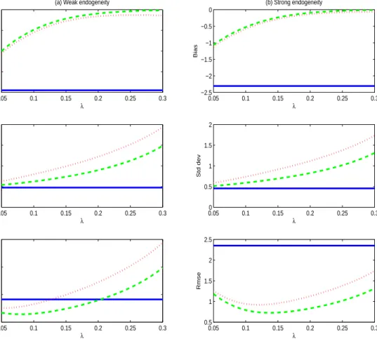
Figs 2 and 3 report bias (Bias), standard deviation (Std dev) and root mean squared error (Rmse) for the three estimates of the intercept and slope parameters, respectively. On the horizontal axis is the truncation parameter(λ) that indicates the integration lower and upper limits of the L2 estimators given by FX−1(λ) and FX−1(1−λ), respectively. The number of
replications is 10,000. The top panel of Figs 2 and 3 reports the bias for each estimator. Under both weak and strong endogeneity, the OLS estimator has non-negligible bias, and theL2 and
bias-corrected estimators have much smaller bias than the OLS estimators for all values of λ. As expected, whenλis small, the latter two estimators are still subject to the distortion of the endogeneity effect ofXi in the tails. But asλincreases, endogeneity bias dies offquickly. The middle panel of Figs 2 and 3 reports the standard deviation of each estimator. Unsurprisingly, the OLS estimator has the least Std dev and the bias-corrected OLS estimator has the largest Std dev. Also as expected, the larger is λ, the less the number of effective observations used in obtaining the L2 and bias-corrected estimators, and the larger the variance of the L2 and
bias-corrected estimators in consequence. The bottom panel of Figs 2 and 3 reports the Rmse of each estimator. Interestingly, in the case of weak endogeneity, the L2 and bias-corrected
estimators outperform OLS in terms of Rmse only for a small degree of truncation. As λ increases, the increase of the Std dev of theL2 and bias-corrected estimators can dominate the
decrease of bias. In sharp contrast, in the case of strong endogeneity, theL2 and bias-corrected
estimators dominate OLS in terms of Rmse for all values of λunder investigation.
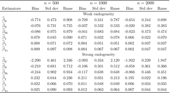
To see the effect of sample size on the various estimators, Table 1 reports the Bias, Std dev, and Rmse for different numbers of observations (n = 500, 1000, and 2000), where the truncation parameter λ takes the value 0.15. The number of replications is 100,000. From Table 1, we see that the endogeneity bias of OLS remains largely unchanged when the sample size is doubled or quadrupled. This is true despite the fact that the support of the location
0.05 0.1 0.15 0.2 0.25 0.3 −0.8 −0.6 −0.4 −0.2 0 λ Bias
(a) Weak endogeneity
0.050 0.1 0.15 0.2 0.25 0.3 0.5 1 1.5 2 λ Std dev 0.05 0.1 0.15 0.2 0.25 0.3 0.5 1 1.5 2 λ Rmse 0.05 0.1 0.15 0.2 0.25 0.3 −2.5 −2 −1.5 −1 −0.5 0 λ Bias (b) Strong endogeneity 0.050 0.1 0.15 0.2 0.25 0.3 0.5 1 1.5 2 λ Std dev 0.05 0.1 0.15 0.2 0.25 0.3 0.5 1 1.5 2 2.5 λ Rmse
Figure 2: Bias, Std dev, and Rmse of various intercept estimators with n=500 observations. OLS estimator (solid line), L2 estimator (dashed line), bias-corrected OLS estimator (dotted
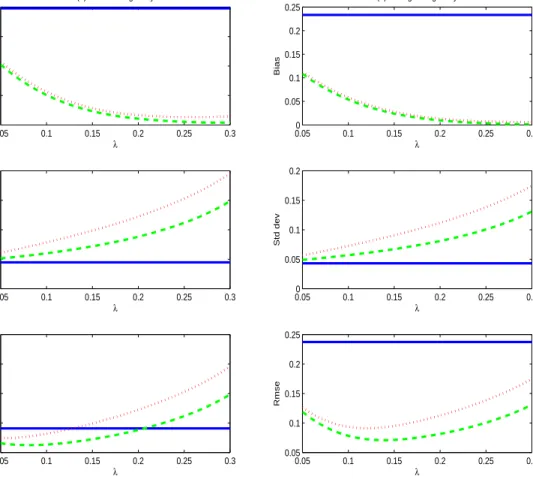
0.050 0.1 0.15 0.2 0.25 0.3 0.02 0.04 0.06 0.08 λ Bias
(a) Weak endogeneity
0.050 0.1 0.15 0.2 0.25 0.3 0.05 0.1 0.15 0.2 λ Std dev 0.05 0.1 0.15 0.2 0.25 0.3 0.05 0.1 0.15 0.2 0.25 λ Rmse 0.050 0.1 0.15 0.2 0.25 0.3 0.05 0.1 0.15 0.2 0.25 λ Bias (b) Strong endogeneity 0.050 0.1 0.15 0.2 0.25 0.3 0.05 0.1 0.15 0.2 λ Std dev 0.05 0.1 0.15 0.2 0.25 0.3 0.05 0.1 0.15 0.2 0.25 λ Rmse
Figure 3: Bias, Std dev, and Rmse of various slope estimators withn=500 observations. OLS estimator (solid line), L2 estimator (dashed line), bias-corrected OLS estimator (dotted line).
Table 1: Comparison of finite sample performance of various estimates
n= 500 n= 1000 n= 2000
Estimators Bias Std dev Rmse Bias Std dev Rmse Bias Std dev Rmse
Weak endogeneity b β0 -0.774 0.473 0.908 -0.709 0.341 0.787 -0.654 0.244 0.698 e β0 -0.076 0.731 0.735 -0.037 0.532 0.533 -0.020 0.382 0.383 b β0c -0.086 0.975 0.979 -0.041 0.683 0.684 -0.023 0.473 0.474 b β1 0.078 0.045 0.090 0.071 0.032 0.078 0.066 0.022 0.070 e β1 0.008 0.071 0.072 0.004 0.051 0.051 0.002 0.037 0.037 b β1c 0.009 0.097 0.098 0.004 0.067 0.067 0.002 0.047 0.047 Strong endogeneity b β0 -2.290 0.461 2.336 -2.093 0.334 2.120 -1.932 0.239 1.947 e β0 -0.210 0.681 0.712 -0.106 0.501 0.512 -0.058 0.361 0.366 b β0c -0.244 0.902 0.934 -0.117 0.638 0.648 -0.066 0.446 0.451 b β1 0.232 0.044 0.236 0.211 0.031 0.213 0.195 0.022 0.196 e β1 0.022 0.066 0.070 0.011 0.048 0.049 0.006 0.034 0.035 b β1c 0.025 0.090 0.093 0.012 0.063 0.064 0.007 0.044 0.044
Note. Corr(ui, uxi) = 0.3 and 0.9 for the case of weak and strong endogeneity, respectively.
shifts is expanding. But since the support expands slowly asnincreases, so too is the reduction of the bias of the OLS estimator. In contrast, both the L2 and bias-corrected OLS estimators
have substantially smaller bias than OLS. As the sample size increases, the bias of the latter two estimators continues to decrease. As expected, the variance of the L2 and bias-corrected
OLS estimators are larger than that of OLS. In terms of Rmse, the L2 estimator generally
dominates the bias-corrected OLS estimator which in turn outperforms OLS.
5
Concluding remarks
The present paper explores a paradox where the greater use of correct prior information on a model can be detrimental in regression. The explanation for this paradox is that even when we use additional correct information about the specification of a model, that information may still not be complete and, in consequence, may distort regression results. In the example studied here, the correct additional information used is considerable and is the full functional form specification of the model. Nevertheless, the omitted information (endogeneity) that makes the model specification incomplete is very important and leads to inconsistency in parametric regression.
In such situations, it is very interesting that partial information can be successful where more complete information fails. In applied statistics, it has long been known that controlling for outliers in regression can help to achieve robustness. What the results of the present
pa-per show, is that nonparametric kernel regression naturally utilizes this mechanism to great advantage in structural regression. More specifically, kernel regression has a considerable ad-ditional advantage beyond its usually touted advantage of robustness to (unknown) functional form. Local nonparametric regression also provides robustness to endogeneity in the regres-sor when there are systematic influences that assure identification, such as location shifts or nonstationarity in the data.
It is also possible to obtain consistent estimation by parametric methods in such cases. In particular, spatialL2 regression is shown to successfully remove endogeneity bias and
inconsis-tency by bounding the domain of the regression. This approach is analogous to the treatment of outliers — it provides protection against possible effects of endogeneity in parametric regression by paying a premium through the loss of tail information in the data.
6
Appendix: Proofs and supplementary technical results
6.1
Proof of Theorem 2.2
Noting that √n(bθ−θ) =¡n−1X0X¢−1n−1/2X0u, we have
√ nDn ³ b θ−θ−¡X0X¢−1E¡X0u¢´ = ¡Dn−1n−1X0XD−n1¢−1Dn−1n−1/2¡X0u−E¡X0u¢¢. We prove the theorem by showing that
Γn≡D−n1n−1X0XD−n1 →p lim n→∞ Ã 1 L−n1μx L−1 n μx 121 + E(u2 xi) L2 n ! ≡Γ, (6.1) and An≡D−n1n−1/2(Xu−E(Xu ))→dN(0,Ω), (6.2) where Ω= lim n→∞ ⎛ ⎝ σ2 E(ux1u21) Ln E(ux1u21) Ln σ2 12+ Var(ux1u1) L2 n ⎞ ⎠. First, by the fact thatX =ux →p μx,and (2.2), we have
L−n2n−1 n X i=1 Xi2 = L−n2n−1 n X i=1 ¡ Xi−X ¢2 +L−n2X2 = 1 12 + σ2 x L2 n + μ 2 x L2 n +oP(1) = 1 12 + E¡u2x1¢ L2 n +oP (1).
Thus (6.1) follows. To show (6.2), by the Cramér-Wold device it suffices to show that for any ω= (ω1, ω2)0 withkωk= 1,we have ω0An=n−1/2 n X i=1 © ω1ui+ω2L−n1[Xiui−E(Xiui)] ª →d N ¡ 0, ω0Ωω¢. (6.3)
By construction,E(ω0An) = 0.We now calculate the asymptotic variance of ω0An: Var¡ω0An ¢ = n−1 n X i=1 Var¡ω1ui+ω2L−n1[Xiui−E(Xiui)] ¢ = ω21σ2+ 2ω1ω2L−n1n−1 n X i=1 E¡Xiu2i ¢ +ω22L−n2n−1 n X i=1 Var(Xiui) → ω0Ωω, because L−1 n n−1 Pn i=1E ¡ Xiu2i ¢ =L−1 n E ¡ uxiu2i ¢ ,and 1 nL2 n n X i=1 Var(Xiui) = 1 (2m+ 1)L2 n m X α=−m 1 M X i∈Aα Var µµ Lnα 2m +uxi ¶ ui ¶ = 1 (2m+ 1)L2 n m X α=−m 1 M X i∈Aα ½ L2nα2 4m2 σ 2+Var(u xiui) + Lnα m E £ uxiu2i ¤¾ = σ 2 (2m+ 1) 2m2 m(m+ 1) (2m+ 1) 6 + Var(uxiui) L2 n → σ 2 12 + limn→∞ Var(uxiui) L2 n .
Letξin =n−1/2©ω1ui+ω2L−n1[Xiui−E(Xiui)]
ª .By theCr inequality, n X i=1 E|ξin|2+δ = 1 n1+δ/2 n X i=1 E¯¯ω1ui+ω2Ln−1[Xiui−E(Xiui)] ¯ ¯2+δ ≤ 2 1+δ n1+δ/2 n X i=1 n E|ω1ui|2+δ+ ¯ ¯ω2L−n1 ¯ ¯2+δ EkXiui−E(Xiui)k2+δ o ≤ 2 1+δ |ω1|2+δ n1+δ/2 n X i=1 E|ui|2+δ+¯¯ω2L−n1 ¯ ¯2+δ 23+2δ n1+δ/2 n X i=1 EkXiuik2+δ = O(n−δ/2) +O((mM)−δ/2) =o(1).
Then (6.3) follows by the Liapounov CLT.
6.2
Proof of Theorem 3.1
For notational simplicity, letKix=Kh(Xi−x).Define Qn= Ã Rb afb(x)dx Rb axfb(x)dx Rb axfb(x)dx Rb a x2fb(x)dx ! . Wefirst prove some lemmas that are used in the proof of Theorem 3.1.
Lemma 6.1 Let Θjn= Rb axjfb(x)dx for j= 0,1,2. Then (i) EΘjn= b j+1−aj+1 j+1 +o(1), (ii) Var(Θjn) =O ³ Ln mM + hL2 n mM ´ =o(1)for j= 0,1,2.
Proof. Recall N = 2mM/Ln and fb(x) =N−1Pni=1Kh(Xi−x).By the Fubini theorem and Taylor expansion,
EΘjn = Ln 2m m X a=−m Z b a Z xjK(z)fux(x−μα+hz)dzdx = Ln 2m m X a=−m Z b a xjfux(x−μα)dx+ h2μ2(K)Ln 2m m X a=−m Z b a xjfu00x(x−μα)dx+Rjn.(6.4) whereRjn= h 2L n 2m Pm a=−m Rb a R R xjz2K(z)£fu00x(x−μα+whz)−fu00x(x−μα)¤(1−w)dwdzdx is the remainder term. Noting
Ln 2m m X a=−m fux(x−μα) ≈ Z Ln/2 Ln/2 fux(x−p)dp→ Z ∞ −∞ fux(x−p)dp= 1, Ln 2m m X a=−m+1 fu00x(x−μα) ≈ Z Ln/2 Ln/2 fu00x(x−p)dp→ Z ∞ −∞ fu00x(x−p)dp <∞,
it follows that the first term in (6.4) tends to
Z b a
xjdx= b
j+1−aj+1
j+ 1 , (6.5)
the second term in (6.4) is approximately h2μ2(K) Z ∞ −∞ fu00x(p)dp Z b a xjdx=O¡h2¢, and Rjn=o ¡ h2¢by dominated convergence.
Now, by Jensen’s inequality, the Fubini theorem, a change of variables, and since (ui, uxi) isiid, we have Var(Θjn) = L 2 n 4m2M2 n X i=1 Var µZ b a xjKh(Xi−x)dx ¶ = L 2 n 4m2M m X a=−m Var µZ b a xjKh(μα+ux1−x)dx ¶ ≤ L 2 n 4m2M m X a=−m Z b a Z b a xjexjE[Kh(μα+ux1−x)Kh(μα+ux1−xe)]dxdex = L 2 n 4m2M m X a=−m Z b a Z b a xjexj Z Kh(μα+ux1−x)Kh(μα+ux1−ex)fux(ux1)dux1dxdex = L 2 n 4hm2M m X a=−m Z b a Z b a xjxej Z K(z)K µ z+x−ex h ¶ fux(x−μα+hz)dzdxdxe = Ln 2hmM Z b a Z b a xjxej Z K(z)K µ z+x−xe h ¶ Ln 2m m X a=−m fux(x−μα)dzdxdxe+O µ hL2n mM ¶ = Ln 2hmM Z b a Z b a xjxej Z K(z)K µ z+x−xe h ¶ dzdxdxe{1 +o(1)}+O µ hL2n mM ¶ = Ln 2mM Z b a Z (b−x)/h (a−x)/h xj(x+hv)j Z K(z)K(z−v)dzdvdx+O µ hL2n mM ¶ = O µ Ln mM + hL2 n mM ¶ . Lemma 6.2 Let Ξjn= Rb aN− 1/2Pn i=1xj(Xi−x)Kixdx for j= 0,1.Then Ξjn=oP(1). Proof. By the Fubini theorem and Taylor expansion,
E(Ξjn) = r M Ln 2m m X a=−m Z b a E£xj(μα+ux1−x)Kh(μα+ux1−x) ¤ dx = r M Ln 2m m X a=−m Z b a Z xjzK(z)fux(x−μα+hz)dzdx = h2 r 2mM Ln μ2(K) (Z b a xjLn 2m m X a=−m fu00x(x−μα)dx{1 +o(1)} ) = h2√N Z b a xjdx Z fu00x(p)dp{1 +o(1)} = o(1).
Analogous to the proof of Lemma 6.1(ii), we can show that Var(Ξjn) = O¡h2¢= o(1). The result follows from the Chebyshev inequality.
Lemma 6.3 Let f(u) denote the p.d.f. of ui.Suppose Assumptions 3 and 4 hold. Then Z uLn 2m m X a=−m [f(u, x−μα)−f(u)]du=O((m/Ln)−2+h2).
Proof. The proof follows from that of Lemma 6.1 in Phillips and Su (2009). The main difference is that2m/Ln here plays the role ofmλ in Phillips and Su (2009).
To prove Theorem 3.1, noticing that if g(x) =β0+β1x, then
Z b a b g(x)fb(x)dx = Z b a N−1 n X i=1 Kh(Xi−x)yidx = Z b a N−1 n X i=1 Kix[β0+β1x+β1(Xi−x) +ui]dx = β0 Z b a b f(x)dx+β1 Z b a xfb(x)dx+β1 Z b a N−1 n X i=1 (Xi−x)Kixdx+ Z b a N−1 n X i=1 Kixuidx, and similarly Z b a xbg(x)fb(x)dx = β0 Z b a xfb(x)dx+β1 Z b a x2fb(x)dx+β1 Z b a N−1 n X i=1 x(Xi−x)Kixdx+ Z b a N−1 n X i=1 xKixuidx. It follows that √ N ³ eθ−θ ´ = β1Q−n1 à Rb aN−1/2 Pn i=1(Xi-x)Kixdx Rb aN− 1/2Pn i=1x(Xi-x)Kixdx ! +Q−n1 à Rb aN−1/2 Pn i=1Kixuidx Rb aN− 1/2Pn i=1xKixuidx ! . (6.6) By Lemma 6.1, Qn→p à b−a b2−2a2 b2−a2 2 b3−a3 3 ! =Q, (6.7)
where det(Q) = (b−a)4/12 > 0 as b 6= a. This, together with Lemma 6.2, implies that the
first term in (6.6) isoP(1).We are left to show that the second term in (6.6) is asymptotically N¡0, σ2Q−1¢.
Let ω= (ω1, ω2)0 be such thatkωk= 1,and define
Θn=ω0 Ã Rb aN− 1/2Pn i=1Kixuidx Rb aN−1/2 Pn i=1xKixuidx ! =N−1/2 n X i=1 Z b a (ω1+ω2x)Kixuidx.
We complete the proof by showing that E(Θn) =O ¡ N1/2h2¢=o(1)by Assumption 6, and Θn−E(Θn)→dN ¡ 0, σ2ω0Qω¢. (6.8) By a change of variables, the Fubini theorem, Lemma 6.3, and Assumptions 1(ii), 3 and 6, we obtain EΘn = r M Ln 2m m X a=−m Z b a E[(ω1+ω2x)Kh(μα+ux1−x)u1]dx = r M Ln 2m m X a=−m Z b a Z Z (ω1+ω2x)uK(z)f(u, x−μα+hz)dzdu dx = r 2mM Ln Z b a (ω1+ω2x) Z K(z) (Z uLn 2m m X a=−m f(u, x−μα+hz)du ) dz dx = √N Z b a (ω1+ω2x) Z K(z) ½ O³(m/Ln)−2+h2´+ Z uf(u)du ¾ dz dx = √N O³(m/Ln)−2+h2 ´ =o(1). Next, lettingw(x) =ω1+ω2x,we have
Var(Θn) = N−1 n X i=1 Var µ ui Z b a (ω1+ω2x)Kixdx ¶ = Ln 2m m X a=−m Z b a Z b a E[w(x)w(xe)u21Kh(μα+ux1−x)Kh(μα+ux1−xe)]dxdex+o(1) = Ln 2m m X a=−m Z b a Z b a w(x)w(xe) Z Z u2Kh(μα+ux−x)Kh(μα+ux−xe)f(u, ux)duxdudxdxe+o(1) = Ln 2m m X a=−m Z b a Z b a w(x)w(xe) Z Z u2K(z)K µ z+x−xe h ¶ f(u, x−μα+hz)dzdu dxdxe+o(1) = Z b a Z b a w(x)w(xe) Z Z u2K(z)K µ z+x−xe h ¶ Ln 2m m X a=−m f(u, x−μα)dzdu dxdex+o(1) = σ2 Z b a Z b a w(x)w(ex) Z K(z)K µ z+x−xe h ¶ dz dxdxe+o(1) = σ2 Z b a Z (b−x)/h (a−x)/h w(x)w(x+hv) Z K(z)K(z−v)dzdv dx+o(1) = σ2 Z b a (ω1+ω2x)2dx+o(1)→σ2ω0Qω,
where we have used the fact that Ln 2m
Pm
a=−mf(u, x−μα) →
R∞
−∞f(u, x−p)dp =f(u). To
independence of (ui, uxi) across i, it suffices to check the Liapounov condition. Let Zi = Zi−E(Zi),whereZi =N−1/2Rab(ω1+ω2x)Kixuidx. Then by the Cr inequality,
n X i=1 E¯¯Zi ¯ ¯2+δ ≤ 21+δN−(1+δ/2) n X i=1 E ¯ ¯ ¯ ¯ui Z b a (ω1+ω2x)Kixdx ¯ ¯ ¯ ¯ 2+δ +21+δN−(1+δ/2) n X i=1 ¯ ¯ ¯ ¯E ∙ ui Z b a (ω1+ω2x)Kixdx ¸¯¯¯ ¯ 2+δ ≡ Ln1+Ln2. First, Ln1 = 21+δN−δ/2 Ln 2m m X a=−m Z Z ¯¯¯ ¯u Z b a w(x)Kh(μα+ux−x)dx ¯ ¯ ¯ ¯ 2+δ f(u, ux)duxdu ≤ cδN−δ/2 Ln 2m m X a=−m Z Z |u|2+δ ¯ ¯ ¯ ¯ Z b a Kh(μα+ux−x)dx ¯ ¯ ¯ ¯ 2+δ f(u, ux)duxdu ≤ cδN−δ/2 Ln 2m m X a=−m Z Z |u|2+δf(u, ux)duxdu = cδN−δ/2E|u|2+δLn(2m+ 1) 2m = O(N−δ/2Ln) =o(1),
wherecδ= 21+δsupa≤|x|≤b|w(x)|2+δ<∞askωk, aandbarefinite. By the Jensen inequality, Ln2 ≤Ln1=o(1).Then by the Liapounov CLT, (6.8) follows, and the proof is complete.
6.3
Proof of Theorem 3.2
RecallN = 2mM/Ln,and Bn=n−1X0X.Noting that 1 n−1Pn i=1 ¡ Xi−X ¢2 à X ec −ec ! =Bn−1 n X i=1 à 0 −Xieui ! , we have √ N³bθc−θ ´ = √nCn ³ bθ−θ´+ 1 n−1Pn i=1 ¡ Xi−X ¢2 √ N Cn à X ec −ec ! = √N B−n1n−1 n X i=1 à ui Xiui−Xiuei ! = √N B−n1n−1 n X i=1 à ui ¡ Xi, Xi2¢ ³eθ−θ´ ! .
Letω = (ω1, ω2)0 with kωk= 1.Define Tn= √ N ω0Bn−1n−1 n X i=1 Ã ui ¡ Xi, Xi2¢ ³eθ−θ ´ ! . By the Cramér-Wold device, it suffices to show that
Tn→dN
¡
0, ω0Ψω¢. (6.9) We show (6.9) by distinguishing whetherLn is allowed to approach∞ asn→ ∞.
Case 1. Ln→ ∞asn→ ∞.Noting that
√ N n−1 =o¡n−1/2¢, X =n−1Pni=1uxi→p μx, L−n2n−1Pni=1Xi2 = L−n2n−1Pni=1¡Xi−X¢2 +Ln−2X2 →p 121, we have √ N n−1Pni=1ui →p 0, Sxnc2 /Sx2 →p 1 and X/Sx2 →p 0, where Sx2 = n−1 Pn i=1 ¡ Xi−X ¢2 and S2xnc = n−1Pni=1Xi2. Also note that
Bn−1 = 1 S2 x à Sxnc2 −X −X 1 ! . (6.10) It follows that Tn = √N n−1ω0 n X i=1 1 S2 x ⎛ ⎝ S 2 xncui−X ¡ Xi, Xi2 ¢0³eθ −θ´ −Xui+¡Xi, Xi2¢0 ³ e θ−θ ´ ⎞ ⎠ = √N n−1 n X i=1 1 S2 x n¡ ω1Sxnc2 −ω2X ¢ ui+ ¡ ω2−ω1X ¢ ¡ Xi, Xi2 ¢0³eθ −θ´o = ω2−ω1X S2 x √ N³eθ−θ´0n−1 n X i=1 à Xi Xi2 ! +oP (1) = ¡ ω2−ω1X ¢√ N³eβ1−β1´ S2 x Sxnc2 + ¡ ω2−ω1X ¢√ N³eβ0−β0´ S2 x X+oP(1) = (ω2−ω1μx) √ N³βe1−β1´+oP(1) →d N ³ 0, σ2(ω2−ω1μx) 2 q22 ´ =N à 0, σ2q22ω0 à μ2x −μx −μx 1 ! ω ! , whereq22 is the (2,2)element ofQ−1 :
Q−1 = 12 (b−a)4 Ã b3−a3 3 − b2−a2 2 −b2−2a2 b−a ! ≡ Ã q11 q12 q21 q22 ! .
Case 2. Ln=Lisfixed asn→ ∞.By the proof of Theorem 3.1 (see (6.6) and arguments thereafter), √ N³eθ−θ´ = Q−1N−1/2 n X i=1 Ã Rb a[Kixui−E(Kixui)]dx Rb ax[Kixui−E(Kixui)]dx ! +oP(1) ≡ n X i=1 Ã ξi1 ξi2 ! +oP(1),
where ξi1 =N−1/2 ½ q11 Z b a [Kixui−E(Kixui)]dx+q12 Z b a x[Kixui−E(Kixui)]dx ¾ , (6.11) and ξi2 =N−1/2 ½ q21 Z b a [Kixui−E(Kixui)]dx+q22 Z b a x[Kixui−E(Kixui)]dx ¾ . (6.12) Let Rn=√N n−1 n X i=1 Ã ui ¡ Xi, Xi2¢ ³eθ−θ´ ! . Then ω0Rn = ω2 √ N ³ e β1−β1 ´( n−1 n X i=1 Xi2 ) +ω2 √ N ³ e β0−β0 ´( n−1 n X i=1 Xi ) +ω1 √ N n−1 n X i=1 ui = ω2cx √ N³βe1−β1´+ω2μx √ N³βe0−β0´+ω1 √ N n−1 n X i=1 ui+oP(1) = n X i=1 ³ ω2cxξi2+ω2μxξi1+ω1 √ N n−1ui ´ +oP(1) ≡ Rn+oP (1),
where recall cx = limn→∞n−1Pni=1E
¡
Xi2¢ = L122 + E(uxi2 ). Let c = (μx, cx)0. Note that E¡Rn ¢ = 0,and Var¡Rn ¢ = n X i=1 Var³ω2cxξi2+ω2μxξi1+ω1 √ N n−1ui ´ = ω22 n X i=1 Var(cxξi2+μxξi1) + 2ω2ω1 n X i=1 Cov ³ cxξi2+μxξi1,√N n−1ui ´ +ω21 n X i=1 Var³√N n−1ui ´ = σ2ω22c0Q−1c+ 2ω2ω1σ2L−1 ½ q11 Z b a dx+q12 Z b a xdx+q21 Z b a dx+q22 Z b a xdx ¾ +ω21σ2L−1+o(1) → σ2ω22c0Q−1c+ 2ω2ω1σ2L−1+ω21σ2L−1 =σ2ω0 Ã L−1 L−1 L−1 c0Q−1c ! ω,
and the following two limits: n X i=1 E ³ ξi1√N n−1ui ´ = n−1 n X i=1 E ½∙ q11 Z b a [Kixui−E(Kixui)]dx+q12 Z b a x[Kixui−E(Kixui)]dx ¸ ui ¾ = q11n−1 n X i=1 E ½ u2i Z b a Kixdx ¾ +q12n−1 n X i=1 E ½ u2i Z b a xKixdx ¾ = q11(2m+ 1)−1 m X α=−m Z b a Z Z u2K(z)f(u, x−uα+hz)dzdudx +q12(2m+ 1)−1 m X α=−m Z b a x Z Z u2K(z)f(u, x−uα+hz)dzdudx = q11L−1 Z b a Z u2 ( L 2m m X α=−m f(u, x−uα) ) dudx{1 +o(1)} +q12L−1 Z b a x Z u2 ( L 2m m X α=−m f(u, x−uα) ) dx{1 +o(1)} = σ2q11L−1 Z b a dx{1 +o(1)}+σ2q12L−1 Z b a xdx{1 +o(1)} → σ2L−1 ½ q11 Z b a dx+q12 Z b a xdx ¾ ; and, in a similar way,
n X i=1 E³ξi2√N n−1ui ´ = n−1 n X i=1 E ∙ q21u2i Z b a Kixuidx+q22u2i Z b a xKixdx ¸ → σ2L−1 ½ q21 Z b a dx+q22 Z b a xdx ¾ .
The Liapounov condition follows from the verification in the proof of Theorem 3.1, the fact that √N n−1Pn
i=1ui also satisfies the Liapounov condition, and the Cr inequality. It follows that Rn→dN Ã 0, σ2 Ã L−1 L−1 L−1 c0Q−1c !! and Tn=ω0Bn−1Rn→dN Ã 0, σ2ω0B−1 Ã L−1 L−1 L−1 c0Q−1c ! B−1ω ! . References
Chen, L-A., A. H. Welsh, and W. Chan (2001) Estimators for the linear regression model based on winsorized observations. Statistica Sinica 11, 147-172.
Hall, P. and J. L., Horowitz (2005) Nonparametric methods for inference in the presence of instrumental variables.Annals of Statistics 33, 2904-2929.
Phillips, P. C. B. and L. Su (2009) Nonparametric structural estimation via continuous loca-tion shifts in an endogenous regressor. Mimeo, Dept. of Economics, Yale University. Wang, Q. and P. C. B., Phillips (2009) Structural nonparametric cointegrating regression.
Forthcoming in Econometrica.