Major Subject: Mathematics May 2006
DOCTOR OF PHILOSOPHY
in partial fulfillment of the requirements for the degree of Texas A&M University
Submitted to the Office of Graduate Studies of EDWARD J. FUSELIER, JR.
by A Dissertation
Major Subject: Mathematics May 2006
Albert Boggess Head of Department Bojan Popov
Joseph E. Pasciak Fred Dahm
Committee Members, Joseph D. Ward Francis J. Narcowich Co-Chairs of Committee,
Approved by:
DOCTOR OF PHILOSOPHY
in partial fulfillment of the requirements for the degree of Texas A&M University
Submitted to the Office of Graduate Studies of EDWARD J. FUSELIER, JR.
by A Dissertation
ABSTRACT
Refined Error Estimates for Matrix-valued Radial Basis Functions. (May 2006) Edward J. Fuselier, Jr., B.S., Southeastern Louisiana University
Co–Chairs of Advisory Committee: Dr. Francis Narcowich Dr. Joe Ward
Radial basis functions (RBFs) are probably best known for their applications to scattered data problems. Until the 1990s, RBF theory only involved functions that were scalar-valued. Matrix-valued RBFs were subsequently introduced by Narcowich and Ward in 1994, when they constructed divergence-free vector-valued functions that interpolate data at scattered points. In 2002, Lowitzsch gave the first error estimates for divergence-free interpolants. However, these estimates are only valid when the target function resides in the native space of the RBF. In this paper we de-velop Sobolev-type error estimates for cases where the target function is less smooth than functions in the native space. In the process of doing this, we give an alternate characterization of the native space, derive improved stability estimates for the in-terpolation matrix, and give divergence-free inin-terpolation and approximation results for band-limited functions. Furthermore, we introduce a new class of matrix-valued RBFs that can be used to produce curl-free interpolants.
TABLE OF CONTENTS
CHAPTER Page
I INTRODUCTION AND PRELIMINARIES . . . 1
A. Introduction . . . 1
B. General Notation . . . 7
C. The Fourier Transform . . . 7
D. Sobolev Spaces . . . 8
1. Scalar-valued Sobolev Spaces . . . 8
2. Vector-valued Sobolev Spaces . . . 9
3. Extension and Trace . . . 10
E. Positive Definite Matrix-Valued Functions . . . 11
II DIVERGENCE-FREE AND CURL-FREE RBFS . . . 14
A. Divergence-free Matrix-Valued RBFs . . . 14
B. Curl-free Matrix-Valued RBFs . . . 14
III NATIVE SPACES FOR MATRIX-VALUED KERNELS. . . 18
A. Native Spaces as Reproducing Kernel Hilbert Spaces . . . 18
B. Alternate Characterizations of Native Spaces . . . 22
C. Native Spaces as Sobolev Spaces . . . 26
D. Generalized Interpolation on Native Spaces . . . 28
IV STABILITY . . . 32
A. Lower Bounds For λmin(AX,Φdiv) . . . 32
B. Lower Bounds For λmin(AX,Φcurl) . . . 41
V BAND-LIMITED INTERPOLATION AND APPROXIMATION 43 A. Divergence-Free and Curl-Free Approximation . . . 43
B. Divergence-Free Band-limited Interpolation . . . 44
C. Curl-Free Band-limited Interpolation . . . 52
VI ERROR ESTIMATES FOR FUNCTIONS OUTSIDE THE NATIVE SPACE . . . 53
A. Extensions of Sobolev Spaces to the Native Space . . . 53
VII CONCLUSIONS AND FUTURE RESEARCH . . . 64
REFERENCES . . . 67
APPENDIX A . . . 71
APPENDIX B . . . 73
LIST OF TABLES
TABLE Page
I Popular Examples of RBFs . . . 1 II Examples of Wendland Functions . . . 12
LIST OF FIGURES
FIGURE Page
1 The Wendland functionφ3,0 onR2. . . 13
2 The Wendland functionφ3,2 onR2. . . 13
3 A two-dimensional divergence-free RBF withφ =φ3,2. . . 15
INTRODUCTION AND PRELIMINARIES A. Introduction
Radial basis functions (RBFs) are probably best known for their applications to scattered data problems. Suppose you are given a finite set of points X ⊂ Rn and data associated with each point and are asked to find a continuous function that fits the data at the points. Given an RBF φ one can build an interpolant out of linear combinations of shifts of φ, i.e., φ generates a “basis” of the approximation space. Also, for RBFs we have φ(x) =φ(kxk), which leads to the name radial basis functions. Such functions do exist, and popular examples include Gaussians, Hardy mulitiquadrics, thin plate splines, and Wendland functions (see Table I and the table on page 12).
Table I. Popular Examples of RBFs
RBF φ(x) Gaussians e−αkxk22, α >0 Hardy Multiquadrics (−1)dβ/2e(c2+kxk2 2)β,β >0,β /∈N Inverse Multiquadrics (−1)dβ/2e(c2+kxk2 2)β,β <0,β /∈N Powers (−1)dβ/2ekxkβ 2,β >0,β /∈2N
Thin Plate Splines (−1)k+1kxk2k
2 log(kxk2), k∈N
Wendland Functions φn,k (see Table II)
Although RBFs were initially studied to solve the interpolation problem, it turns out their applications are much more broad. RBFs can also fit data coming from a
very large class of continuous linear functionals. In particular, they can interpolate derivative and integral data at any point, and therefore can be used to solve partial differential equations numerically. Furthermore, one can use scalar-valued RBFs to build functions that produce vector-valued interpolants with certain physical proper-ties, such as being divergence-free or curl-free.
Hardy was probably the first to study RBFs for the purpose of scattered data interpolation in the early 1970s. He used the so-calledHardy multiquadricsto approx-imate topographical surfaces [9]. In the late 1970s, Duchon studied the approximation properties of the thin plate spline [5, 6]. Throughout the 1980s, important aspects to the theory were solved, such as the existence and uniqueness of RBF interpolants [17, 18]. With the rise of computational power in the 1990s, RBFs became more popular, and they are now being used for many applications, including computer animation, medical imaging, and fluid dynamics [1, 10, 11, 13, 16].
Until the 1990s, RBF theory only involved functions that were scalar-valued. However, many physical applications involve vector fields that are divergence-free or curl-free, so there was interest in using RBFs to construct vector-valued approxima-tions with similar characteristics. Matrix-valued RBFs were subsequently introduced by Narcowich and Ward in 1994 [22]. They constructed matrix-valued functions that yield divergence-free interpolants at scattered points. Constructing such functions turns out to be fairly simple. If φ is a scalar-valued function consider
Φdiv := −∆I +∇∇Tφ,
where∇is then×1 gradient operator and ∆ = ∇T∇is the Laplacian operator. This is ann×nmatrix-valued function with divergence-free columns. Ifφis an RBF, then this function can be used to produce divergence-free interpolants. We note that Φdiv is not a radial function, but because it is usually generated by an RBF φ, it is still
One builds a divergence-free interpolant in the following way. Given a finite point set X ={xj}N
j=1 ⊂Rn and data dj ∈ Rn associated with each xj, we look for
coefficient vectors{cj}Nj=1 ⊂Rn so that
N
X
j=1
Φdiv(xk−xj)cj =dk ∀k = 1, . . . , N. This leads to the matrix equation
AX,Φdivc=d, (1.1)
where c and d are nN ×1 vectors whose jth n components are given by cj and dj, respectively. Also,AX,Φdiv is an nN ×nN matrix whose (j, k)
th n×n block is given by Φdiv(xj−xk). This matrix is symmetric and positive definite, so (1.1) has a unique solution.
In 2002, Lowitzsch [14] gave the first error estimates for the divergence-free in-terpolants, at least in the case where the data is given by an underlying function with a particular smoothness. She also gave stability estimates for the interpolation process, and used the divergence-free RBFs to successfully model a physical problem described by the Navier-Stokes equation [16].
Matrix-valued RBF theory is quite new, so there is much room for improvement. Much has been discussed about divergence-free functions, but their counterpart, curl-free functions, have not been dealt with yet. In this paper we will address this issue by introducing a class of functions that yield curl-free interpolants. We will see that many of the results we will prove for divergence-free RBFs will carry over to the curl-free case.
Another issue that needs to be resolved is the current error estimates. In order to discuss this further, we need to introduce the idea of the native space. Each scalar RBF φ gives rise to a space of functions called the native space of φ, denoted Nφ. In the scalar case, these are Hilbert spaces with an inner product (·,·)Nφ such that if f ∈ Nφ, then (f, φ(·−y))Nφ =f(y). There is an analogue of this in the matrix-valued theory. The error estimates given in [14] are only valid for classes of functions within these native spaces. Native spaces are usually comprised of functions which are very smooth and tend to be small, so such error estimates are quite limited. Our main goal here is to show that the approximation properties of matrix-valued RBFs extend to functions rougher than those in the native space. Finding such estimates for functions outside the native space is sometimes referred to as “escaping” the native space.
Even for scalar-valued RBFs, this is a very recent development. The first “es-cape” was made by Narowich and Ward in 2002 concerning functions on the n-sphere using spherical basis functions (SBFs), which are positive definite functions on the sphere [23]. Results for RBFs on Rn soon followed [2, 24, 25]. We refer the reader to [19] for a comprehensive overview of these findings. Due to applications to PDEs, it is desirable to obtain error estimates in terms of Sobolev norms. The above findings address this partially, but they only have the appropriate norms on one side of the estimate. However, this issue has recently been completely resolved by Narcowich, Ward, and Wendland for a large class of RBFs, Wendland functions and thin plate splines in particular [26]. Our strategy will be largely based on their approach, and the estimates we present will be of the form
kf−IXfkHk(Ω) ≤hτ−kX,ΩkfkHτ(Ω),
where k ≤ τ is an integer, IXf is the RBF interpolant to the target function f on the point set X. Here hX,Ω represents the mesh norm, which we will define later.
notation and state the necessary definitions. The Fourier transform and its inverse are crucial tools in RBF theory, so we give their definitions. Next we discuss Sobolev spaces and some notions concerning Sobolev spaces, such as extensions and trace. Finally we give the definition of matrix-valued positive definite functions and give a brief introduction to RBFs.
In chapter II we will discuss two important classes of matrix-valued RBFs. First we mention divergence-free RBFs. Next we introduce a new class of matrix-valued RBFs, which can be used to produce curl-free interpolants. We finish the chapter by proving that the functions constructed are strictly positive definite.
We will present results on native spaces for matrix-valued kernels in chapter III. While these native spaces were already defined in [14], our presentation here follows the treatment of native spaces for scalar-valued functions found in [30]. We will begin by giving the definition of areproducing kernel Hilbert space (RKHS) and define the native space for a positive definite matrix-valued function. Next we present a uniqueness result, which will allow us to give more useful characterizations native spaces. In particular, we will use the Fourier transform and show that the native space of certain kernels is comprised of functions with a specific smoothness. When the Fourier transform of φ has algebraic decay, which is the case with Wendland functions, we will get “sobolev-like” spaces. We end this chapter with a discussion of generalized interpolation on native spaces. This has already dealt with in [14], but it was proved for a different definition of the native space. Our result will show that the two definitions are in fact equivalent.
Perhaps surprisingly, stability plays a crucial role in the escape process. In chapter IV we explore the stability of the interpolation matrix through its spectral condition number. As done in [16] and [22], we do this by estimating the norm of the
inverse of AX,Φ. Since the interpolation matrix is symmetric and positive definite,
this amounts to bounding its lowest eigenvalue, λmin(AX,Φ), from below. The way
this is usually done is by finding a matrix-valued function Ψ such that N X j,k=1 α∗jΦ(xj−xk)αk≥ N X j,k=1 α∗jΨ(xj−xk)αk ≥λkαk2,
where αj ∈ Cn and α ∈ CnN with the jth n elements of α given by αj. Such a λ is obviously a lower bound forλmin(AX,Φ). In [16] and [22], this was done for
divergence-free matrix valued functions and λ was found not to depend on N, but only on the dimension n and the minimum separation radius of X, denotedqX. We will choose a Ψ different than that used in [16] and [22] and obtain slightly improved results.
We will discuss band-limited functions in chapter V. In the scalar theory, the final escape of the native space in [26] was made by using the approximation properties of band-limited functions, which are functions in L2 whose Fourier transforms are
compactly supported. These functions are analytic, and their smoothness puts them in most native spaces. We will show that band-limited functions can simultaneously approximateand interpolate both functions in the native space and rougher functions, enabling one to eventually use a triangle inequality to escape the native space.
In this chapter VI we present the main result of the paper, which is to show that interpolants rising from matrix-valued RBFs can approximate functions that are more rough than those in the native space. We begin the chapter with a discussion on extending Sobolev functions from a bounded domain Ω⊂Rn to the native space. Once a function is extended to the native space, best approximation properties of interpolants can be used to help estimate the error. The error estimates we give are in terms of themesh norm. Given a compact set Ω⊂Rnand a finite set X ⊂Ω, the
hX,Ω := sup
x∈Ω
inf xj∈Xk
x−xjk2.
As stated before, the norms involved in the estimates will be Sobolev norms.
Finally, we end with a brief summary in chapter VII. We also include some possible problems for further study.
B. General Notation
We will use the usual multi-index notation: Let α = (α1, . . . , αn) be an n-tuple of nonnegative integers and define|α|:=Pjαj. We will usekxk2 to denote the standard
euclidean norm of x ∈Rn. If f is a matrix-valued function or distribution, we write f∗ for the conjugate transpose off, i.e., f∗ = ¯fT. We define theceiling function dxe to be the function that returns the integer k such that k−1< x≤ k, and the floor function bxc to be the functions that returns the integer k such that k ≤x < k+ 1. Also, we let (x)+=x if x≥0 and 0 otherwise.
Let Ω⊆Rn and f : Ω→R. We will say f ∈Ck(Ω) if f is k-times continuously differentiable. Lp spaces are defined in the usual way: we say f ∈Lp(Ω) if
R Ω|f|
pdx is finite. In the case Ω =Rn, we defineCk:=Ck(Rn) and Lp :=Lp(Rn). Also, iff is vector-valued, we say that f ∈ Ck(Ω) or f ∈Lp(Ω) if each of its components are in Ck(Ω) or Lp(Ω), respectively. This should cause no confusion.
C. The Fourier Transform
The Fourier transform plays an important role in the theory of RBFs. We will use the following convention for the Fourier transform of a function or tempered distribution:
b
f(ξ) :=
Z Rn
and let theinverse Fourier transformof a function or tempered distribution be defined by ˇ f(x) := 1 (2π)n Z Rn f(ξ)eiξTxdξ.
Iff is a matrix-valued function, we will take fbto be the matrix of Fourier transforms of each component of f.
D. Sobolev Spaces
1. Scalar-valued Sobolev Spaces
The error estimates will deal with vector-valued functions whose components reside in Sobolev spaces, which we define now. Let Ω be an open domain inRn, 1≤p < ∞, and kbe a non-negative integer. Supposeuis locally integrable and that the distributional derivatives Dαu exist for all|α| ≤k. Then we define the Sobolev norm to be
kukWk p(Ω) := X |α|≤k kDαukp Lp(Ω) 1/p .
For the casep=∞we have
kukWk
∞(Ω) := max|α|≤kkD αuk
L∞(Ω).
We define the Sobolev spaces to be Wpk(Ω) := n u∈L1loc(Ω) :kukWk p(Ω)<∞ o .
It is also possible to have Sobolev spaces of fractional order. Let 1≤ p <∞, k be a non-negative integer, and 0 < t < 1. We define the Sobolev space Wk+t
kukWpk+t(Ω) := kukpWk p(Ω)+ X |α|=k Z ω Z Ω |Dαu(x)−Dαu(y)|p |x−y|n+pt dxdy 1/p .
In the special casep= 2, we defineHτ(Ω):=Wτ
2(Ω). It is well-known thatHτ(Ω)
is a Hilbert space, and that in the case of Ω =Rn, we may use the Fourier transform to characterizeHτ(Rn): Hτ(Rn) :=nu∈L 2(Rn) :u(b ·) 1 +k · k22 τ /2 ∈L2(Rn) o .
The inner product in Hτ(Rn) is given by
hg, fiHτ(Rn) = Z
Rn
(1 +kξk2
2)τf(ξ)b bg(ξ)dξ.
2. Vector-valued Sobolev Spaces
Let u : Ω → Rn, with uj denoting the jth coordinate of u. If uj ∈ Wk
p(Ω) for all j = 1, . . . , n, then we say u ∈ (Wk
p(Ω))n. We impose the following norms on u∈(Wk p(Ω))n for 1≤p <∞: |u|(Wk p(Ω))n := n X j=1 |uj|pWk p(Ω) !1/p , kuk(Wk p(Ω))n := n X j=1 kujkpWk p(Ω) !1/p . Forp=∞ we have: |u|(Wk ∞(Ω))n := max1≤j≤n|uj|W∞k(Ω), kuk(W∞k(Ω))n := max1≤j≤nkujkW∞k(Ω).
Note that (Hτ(Ω))n is a Hilbert space, and in the special case Ω = Rn the inner product can be defined by
hg, fi(Hτ(Rn))n = Z
Rn
(1 +kξk2
When the context is clear, we will use the notationHτ(Ω) = (Hτ(Ω))n. This should cause no confusion.
We will also be interested in spaces that are divergence-free or curl-free. A function is divergence-free if and only if∇ ·f = 0. Forτ ≥0, we define space
Hdivτ (Ω) :={f ∈Hτ(Ω) : ∇ ·f = 0}. This is a closed subspace of Hτ(Ω).
We would like to define a similar space for curl-free functions. In the casen = 2, a functionf iscurl-free if and only if ∂f2/∂x−∂f1/∂y = 0. When n= 3, a function
f is curl-free if and only if ∇ ×f = 0. We will use the sloppy notation ∇ ×f to represent the curl of a vector field if n= 2. Thus for n= 2 or 3 we define
Hcurlτ (Ω) :={f ∈Hτ(Ω) :∇ ×f = 0}.
This is also a closed subspace of Hτ(Ω). When n > 3, there is no simple analogue for curl involving a nice differential operator. However, using differential forms and Poincar´e’s Lemma we see that a vector-valued function on a manifold has no rotation if and only if it is the differential of a scalar valued function. Therefore for general n we will say a function f ∈ Hτ(Rn) is curl-free on Rn if and only if there is a scalar-valued function in Hτ+1(Rn)/R such that ∇φ=f.
3. Extension and Trace Let Ω⊂Rn, and letf ∈Wτ
p(Ω). Two concepts we will need are that of extendingfto Wτ
p(Rn) and extendingf to the boundary of Ω, denoted by∂Ω. If Ω has a Lipschitz boundary and satisfies an interior cone condition, there is a continuous extension
kEfkWτ
p(Rn) ≤CkfkWpτ(Ω).
Also, the same operator works for all Sobolev spaces Wτ
p(Ω). The operator was produced by Stein for integerτ in [27] and extended to fractional τ later (for a proof of the fractional case, see [4]). We will refer to this operator as Stein’s operator When f is vector-valued, we will let Ef denote Stein’s operator acting on each component
of f.
Another important idea is that of atrace, which one gets by extending a Sobolev function to the boundary of its domain. It is well-known that when∂Ω is Lipschitz, the trace exists and is continuous in the following way
kf|∂ΩkWτ−1/p
p (∂Ω) ≤CkfkW τ p(Ω).
These notions will be especially important in chapter VI.
E. Positive Definite Matrix-Valued Functions
An m ×m matrix-valued function Φ is positive definite on Rn if given any finite, distinct set of points X :={x1, . . . , xN} ⊂Rn we have
X
j,k
αTjΦ(xj −xk)αk ≥0
for all α1, . . . , αN in Rm. If the inequality is strict when αi 6= 0 for some i, then we say the Φ is strictly positive definite (SPD). This is equivalent to saying that the mN×mN matrix whose (j, k)thm×mblock is given by Φ(xj−xk) is positive definite, and hence invertible. We will denote this matrix by AX,Φ. In this paper we will only
Whenm = 1, we get the special case of scalar-valued positive definite functions. A positive definite function φ that depends only on the length of its argument, i.e., φ(x) =φ(kxk2), is called a Radial Basis function (RBF). Some popular examples are
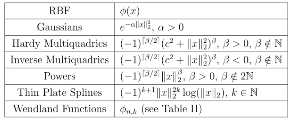
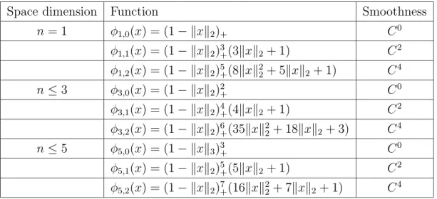
given in Table 1. Wendland functions are particularly important because they are piecewise polynomials with compact support, and are hence easy to compute. We will letφn,k denote the Wendland function that is 2k times continuously differentiable and is positive definite on Rn. Table II lists several of these functions. Examples of Wendland functions are graphed in Figures 1 and 2.
Table II. Examples of Wendland Functions
Space dimension Function Smoothness
n= 1 φ1,0(x) = (1− kxk2)+ C0 φ1,1(x) = (1− kxk2)3+(3kxk2+ 1) C2 φ1,2(x) = (1− kxk2)5+(8kxk22+ 5kxk2+ 1) C4 n ≤3 φ3,0(x) = (1− kxk2)2+ C0 φ3,1(x) = (1− kxk2)4+(4kxk2+ 1) C2 φ3,2(x) = (1− kxk2)6+(35kxk22+ 18kxk2+ 3) C4 n ≤5 φ5,0(x) = (1− kxk3)3+ C0 φ5,1(x) = (1− kxk2)5+(5kxk2+ 1) C2 φ5,2(x) = (1− kxk2)7+(16kxk22+ 7kxk2+ 1) C4
−1 −0.5 0 0.5 1 −1 −0.5 0 0.5 1 0 0.2 0.4 0.6 0.8 1 x axis y axis
Fig. 1. The Wendland function φ3,0 onR2.
−1 −0.5 0 0.5 1 −1 −0.5 0 0.5 1 0 0.5 1 1.5 2 2.5 3 x axis y axis
CHAPTER II
DIVERGENCE-FREE AND CURL-FREE RBFS
In this chapter we will discuss two important classes of matrix-valued RBFs. First we briefly mention divergence-free RBFs. Next we introduce matrix-valued RBFs which can be used to produce curl-free interpolants. We finish the chapter by proving that the curl-free RBFs are positive definite.
A. Divergence-free Matrix-Valued RBFs
Matrix-valued RBFs which yieldC∞divergence-free interpolants were first introduced by Narcowich and Ward in 1994. In 2002, Lowisitzch introduced a class of these functions which areC2kand compactly supported. Constructing such functions turns out to be fairly simple. If φ is a scalar-valued function consider
Φdiv := −∆I+∇∇Tφ,
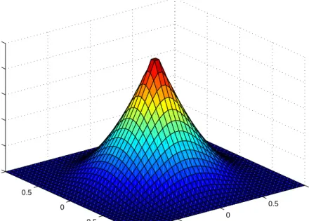
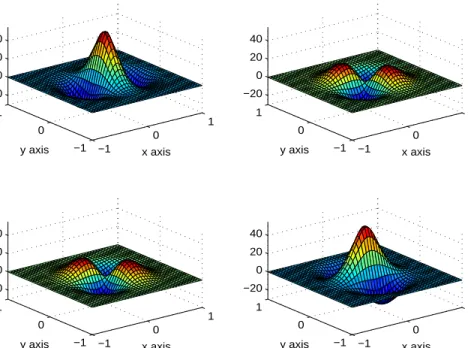
where∇is then×1 gradient operator and ∆ =∇T∇is the Laplacian operator. Then Φdiv is ann×n matrix-valued function with divergence-free columns. If φ is positive definite, then this function can be used to produce divergence-free interpolants. An example of a compactly supported divergence-free RBF is shown in Figure 3.
B. Curl-free Matrix-Valued RBFs
We now present curl-free matrix-valued RBFs. As in the divergence-free case, they are easy to produce. Again we chose a positive definite scalar-valued function and act on it with the appropriate differential operator. Given φ ∈C2, define
−1 0 1 −1 0 1 −20 0 20 40 x axis y axis −1 0 1 −1 0 1 −20 0 20 40 x axis y axis −1 0 1 −1 0 1 −20 0 20 40 x axis y axis −1 0 1 −1 0 1 −20 0 20 40 x axis y axis
Fig. 3. A two-dimensional divergence-free RBF with φ =φ3,2.
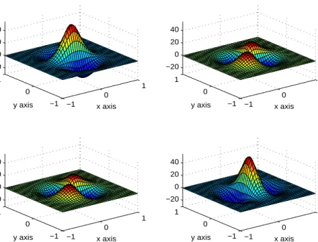
It is easy to see that the columns of this function are curl-free. The jth column is given by Φcurlej, where ej is the standard basis vector with a one in the jth position. This gives us
Φcurlej =−∇∇Tφej =∇ −∇T(φej)=∇g,
where g = −∂φ/∂xj, which is a scalar function. Since the column is the gradient of a scalar, it is curl-free. An example of a curl-free RBF is shown in Figure 4.
To see that Φcurl is positive definite, we will use the Fourier transform and its inverse. In order to be rigorous, we must assume that φ, −∆φ, and their Fourier transforms are in C ∩ L1. This enables us to recover Φ from Φ using the inverseb
−1 0 1 −1 0 1 −20 0 20 40 x axis y axis −1 0 1 −1 0 1 −20 0 20 40 x axis y axis −1 0 1 −1 0 1 −20 0 20 40 x axis y axis −1 0 1 −1 0 1 −20 0 20 40 x axis y axis
Fig. 4. A two-dimensional curl-free RBF with φ=φ3,2.
Fourier transform. cTAX,Φcurlc= X j,k cTjΦcurl(xj −xk)ck =X j,k cTj Z Rn [ ΦcurleixTjξe−ixTkξdξ ck = Z Rn X j cje−ix T jξ !∗ ξξTφb X k cke−ix T kξ ! dξ = Z Rn X j ξTcje−ixTjξ 2 b φ dξ ≥0. (2.1)
This shows that Φcurl is positive definite. To see when it is strictly positive definite, we will need the following lemma.
Lemma 1. Let X = {xj}N
j=1 and {cj}Nj=1 be finite subsets of Rn, and let U be an
open subset of Rn. If the function f(ξ) = P jξTcje
ixT
jξ is zero on U then cj = 0 for
and identically zero on an open subset of Rn, it must be zero on all of Rn. Now let g be any function in L1 such that g and its first derivatives can be recovered by the
inverse Fourier transform and consider: 0 =f(ξ)bg(ξ) = X j ξTcjeixTjξbg(ξ) = X j ∇T(g(· −xj)cj) !ˆ =⇒ X j X i cji ∂ ∂xi g(· −xj)≡0, wherecji is theithcoordinate ofcj. We will show thatc
11= 0, and the rest are proved
similarly. To do this, we chooseg to have compact support withing the ball of radius <min
j6=k kxj−xkk, and that at the origin ∂g/∂x1 = 1 and ∂g/∂xj = 0 for all j 6= 1. For a concrete example that such ag exists, one can use Hermite-Birkoff interpolation to find a linear combination of Wendland functions with those properties. Applying this to the above equation gives us the result.
Applying the lemma to (2.1), we see that if φbis continuous, then Φcurl is strictly positive definite. This almost proves the following theorem.
Theorem 1. Let φ ∈ C2 be a scalar-valued strictly positive definite function on Rn such thatφand−∆φ are inL1. ThenΦcurl is a strictly positive definite matrix-valued
function with columns that are curl-free.
Proof. We need only show that if φ∈C2 be a scalar-valued positive definite function
onRn such that φ and−∆φ are inL
1, then we can recover them through the inverse
Fourier transform. This will happen if the Fourier transforms of φ and −∆φ are in L1. Since φ is positive definite, by Bochner’s theorem so is −∆φ. Now we use [30,
Corollary 6.12], which says that if a positive definite function is continuous and L1
CHAPTER III
NATIVE SPACES FOR MATRIX-VALUED KERNELS
While native spaces were defined with distributions in [14], our presentation here follows the treatment of native spaces for scalar-valued functions found in [30]. We will begin by giving the definition of areproducing kernel Hilbert space (RKHS) and define the native space for a positive definite matrix-valued function. Next we offer a uniqueness result. This feature will allow us to give a more useful characterization of the native space. In particular, we will use the Fourier transform and show that the native space of certain kernels is comprised of functions with a specific smoothness. When the Fourier transform ofφhas algebraic decay, which is the case with Wendland functions, we will get “Sobolev-like” spaces.
In the last section we will deal with generalized interpolation on native spaces. The has already been done in the case where native spaces were defined distribution-ally, but it has not been shown for the definition of the native space given here. In the process of proving this we will show that the two definitions are equivalent.
A. Native Spaces as Reproducing Kernel Hilbert Spaces
An important idea in the theory of RBFs is that of a reproducing kernel Hilbert space, which we define now.
Definition 1. Let F be a Hilbert space of vector-valued functions f : Ω → Rn. A continuousn×n matrix-valued function Φ is called a reproducing kernel for F if for all x∈Ω andc∈Rn we have
1. Φ(· −x)c∈ F.
no restriction on Ω in the definition. However, in the context of RBFs one usually assumes that Ω =Rn.
The first property of the definition tells us that such an F would contain all functions of the form f =PNj=1Φ(x−xj)αj, where αj ∈Rn and xj ∈Ω. The second property gives us an expression for the norm of such functions:
kfk2F = N X k=1 N X j=1 α∗jΦ(xj−xk)αk.
These features will guide us in the construction of a RKHS for a given SPD matrix-valued function. Encouraged by this, we define the space
FΦ(Ω) := ( N X j=1 Φ(· −xj)αj :xj ∈Ω, αj ∈Rn, and N ∈N ) .
We furnish this space with the bilinear form N X j=1 Φ(· −xj)αj, M X k=1 Φ(· −yk)βk ! Φ := N X j=1 M X k=1 βkTΦ(yk−xj)αj. If Φ is SPD then this bilinear form defines an inner product on FΦ(Ω).
We will denote the completion ofFΦ(Ω) with respect to thek·kΦnorm asFΦ(Ω).
The elements of FΦ(Ω) are abstract, and we wish to interpret them as functions. To
do this we define function values for an element f byfj(x) := (f,Φ(· −x)ej)Φ. Will
will show that this leads to an injective linear mapping R :FΦ(Ω) →C(Ω) given by
R(f)j(x) := (f,Φ(· −x)ej)Φ. The image of this map is the space of functions we are
looking for.
Lemma 2. The mapping R:FΦ(Ω)→C(Ω) is an injective linear map.
continuous. We have
|R(f)j(x)−R(f)j(y)|=(f,Φ(· −x)ej)Φ−(f,Φ(· −y)ej)Φ =(f,Φ(· −x)ej −Φ(· −y)ej)Φ
≤ kfkΦkΦ(· −x)ej −Φ(· −y)ejkΦ.
To conclude that R(f)j is continuous, we use the continuity of Φ and the fact that
kΦ(· −x)ej−Φ(· −y)ejk2
Φ = 2eTjΦ(0)ej−eTjΦ(x−y)ej −eTjΦ(y−x)ej. For injectivity, suppose R(f) = 0 for some f ∈ FΦ(Ω). This means that ∀x∈Ω and
all c∈Rn we have (f,Φ(· −x)c)
Φ = 0. Thusf is perpendicular to FΦ, but FΦ is the
completion of FΦ, so f = 0 and R is injective.
With this result, we are able to define the native space.
Definition 2. The native Hilbert function space corresponding to the SPD kernel Φ is defined by
NΦ(Ω) :=R(FΦ(Ω)).
It is equipped with the inner product
(f, g)NΦ(Ω) := (R−1f, R−1g)FΦ(Ω).
Defined in this way, we see that the native space is indeed a Hilbert space of continuous functions with reproduction kernel Φ. To see this, since Φ(· −x)c is mapped to itself throughR for all x∈Ω andc∈Rn, we get
fj(x) = R−1f,Φ(· −x)ejΦ = (f,Φ(· −x)ej)NΦ
for all f ∈ NΦ. One can also use the fact that FΦ(Ω) is dense in NΦ with kfkΦ =
Theorem 2. Suppose thatΦis a SPD matrix-valued kernel. Suppose further thatGis a Hilbert space of functions f : Ω→Rn with reproducing kernel Φ. Then G =N
Φ(Ω)
and the inner products are the same.
Proof. From the remarks after Definition 1, we know that FΦ(Ω) ⊆ G and kfkG =
kfkNΦ(Ω) for allf ∈FΦ(Ω). Letf ∈ NΦ(Ω). By density ofFΦ(Ω) in the native space,
there is a Cauchy sequence {fn} inFΦ(Ω) converging to f in NΦ(Ω). One can show
that if a sequence converges in a RKHS, then it converges point-wise. Indeed if Φ is the reproducing kernel for the RKHS F, we have
|(fn)j(y)−fj(y)|=
(fn−f,Φ(· −y)ej)F
≤ kfn−fkFkΦ(· −y)ejkF. Thus we get f(y) = lim
n→∞fn(y). Note that {fn} is also a Cauchy sequence in G, so it also converges to a g ∈ G. The reproducing-kernel property of G gives g(y) =
lim
n→∞fn(y) =f(y). Therefore f =g ∈ G, so NΦ(Ω) ⊆ G and kfkNΦ(Ω) =kfkG for all f ∈ NΦ(Ω).
Now suppose that NΦ(Ω) is not equal to G. Then we can find an element g ∈
G \ {0} orthogonal to NΦ(Ω). However, since Φ(· −y)ej ∈ NΦ this means that
gj(y) = (g,Φ(· −y)ej)G = 0 for all y∈ Ω and all j = 1, . . . , n. Thus NΦ(Ω) =G. To
finish the proof, by polarization we know that the inner products are equal because the norms are.
This feature will give us the tools to give other characterizations of the native space in the next section. In particular, we will use the Fourier transform and show that the native space of certain kernels is comprised of functions with a specific smoothness.
B. Alternate Characterizations of Native Spaces
In the theory of scalar-valued positive definite functions, it is well-known that in the case of φ∈C(Rn)∩L
1(Rn), one may characterize the native space of φ by
Nφ(Rn) = ( f ∈L2 ∩C : Z Rn |fb(ξ)|2 b φ(ξ) dξ <∞ ) ,
with inner product given by
(f, g)Nφ(Rn) := (2π)−n/2 Z Rn b g(ξ)f(ξ)b b φ(ξ) dξ. (3.1)
IfΦ(ξ) is invertible for allb ξ, an appropriate guess for the generalization of (3.1) would be
(f, g)NΦ(Rn) := (2π)−n/2 Z
Rnb
g(ξ)∗Φ(ξ)b −1f(ξ)dξ.b
However, Φdivd and Φcurl[ are not invertible at any point. Nevertheless we get around this obstruction by considering theMoore-Penrose inverse, orpseudo-inverse, ofΦ(ξ),b which we denote by Φ(ξ)b +. Thus a more appropriate inner product would be
(f, g)NΦ(Rn) := (2π)−n/2 Z
Rnb
g(ξ)∗Φ(ξ)b +f(ξ)dξ.b
Also, to make sure the inner product is strictly positive definite, one should be careful about what functions are allowed in the space. In particular, we should avoid those whose Fourier transforms are perpendicular to the columns of Φ(ξ)b +.
In the case of divergence-free and curl-free matrix-valued functions, a simple calculation gives us the following equalities:
d Φdiv(ξ)+= 1 kξk2 2φ(ξ)b I−eξeTξ [ Φcurl(ξ)+= 1 kξk2 2φ(ξ)b eξeTξ,
the identity for the Fourier transforms of functions in the native space. Therefore in the divergence-free case, we will consider functions f such that eT
ξfb(ξ) = 0. In the curl-free case we want functions of the form f(ξ) =b eξh(ξ), where his a scalar-valued function. Now we are ready to state and prove the following results.
Theorem 3. Suppose that φ∈C2 is a positive definite function such that ∆φ ∈L 1. Define Gdiv := f ∈L2∩C : Z Rn b
f(ξ)∗Φdiv(ξ)d +f(ξ)dξ <b ∞ and eTξfb(ξ) = 0 a.e.
and equip this space with the bilinear form (f, g)Gdiv := (2π)−n/2
Z Rnb
g(ξ)∗Φddiv(ξ)+fb(ξ)dξ.
Then Gdiv is a Hilbert space with inner product (·,·)Gdiv and reproducing kernel Φdiv.
Hence Gdiv =NΦdiv and the inner products are the same.
Proof. We begin by noting that since f ∈ Gdiv satisfies eTξfb(ξ) = 0 for all ξ, we have (f, f)Gdiv = (2π)−n/2 Z Rn kf(ξ)b k2 2 kξk2 2φ(ξ)b dξ. (3.2)
Also, sinceφ is positive definite so is −∆φ. Then that fact that it is continuous and L1 integrable puts its Fourier transform is in L1(Rn) [30, Corollary 6.12]. This
means thatfb∈L1 for all f ∈ Gdiv. Indeed, we have Z Rn| b fj(ξ)|dξ ≤ Z Rn |fjb(ξ)|2 2 kξk2 2φ(ξ)b dξ !1/2Z Rnk ξk22φ(ξ)dξb 1/2 .
This allows us to recoverf point-wise from its Fourier transform by the inverse Fourier transform.
symmetry properties are obvious. The fact thatφbis positive along with (3.2) tells us (f, f)Gdiv = 0 implies thatf = 0. Thus (·,·)Gdiv is positive definite and hence an inner
product.
To show completeness of Gdiv, suppose that {fn} is a Cauchy sequence in Gdiv. This means that the sequence nfbn(k · k22φ)b −1/2
o
is Cauchy inL2, and so it converges
to a functiong ∈L2. Note that the functiong satisfiesg q k · k2 2φb∈L1∩L2. Namely, Z Rn gj(ξ) q kξk2 2φ(ξ)b dξ ≤ kgjkL2 k · k2 2φb 1/2 L1 and Z Rn gj(ξ) q kξk2 2φ(ξ)b 2 dξ ≤ kgjk2L2k · k22φb L∞. for all j = 1, . . . , n. Thus
f(x) := (2π)−n/2 Z Rn g(ξ) q kξk2 2φ(ξ)b eixTξdξ
is well defined, continuous, an element of L2, and satisfies b
f(k · k22φ)b −1/2 =g ∈L2. (3.3)
Note that sincegis theL2 limit of the sequence n b fn(k · k2 2φ)b −1/2 o ,gsatisfieseT ξg(ξ) = 0 a.e. This is because eT
ξfn(b k · k22φ)b −1/2 tends to eTξg(ξ) in L2 as n tends to ∞, and
the former is a sequence of zeros. Then by (3.3), the Fourier transform of f satisfies the orthogonality condition. Therefore f resides in Gdiv. Now we have that
kfn−fk2Gdiv = (2π)
−n/4kfb
n(k · k22φ)b −1/2−fb(k · k22φ)b −1/2kL2
= (2π)−n/4kfn(b k · k2
2φ)b −1/2−gkL2 →0
as n tends to ∞. We conclude that Gdiv is complete.
(f,Φdiv(· −y)c) = (2π)−n/2
Z Rn
d
Φdiv(ξ)ce−iξTy∗Φdiv(ξ)d +fb(ξ)dξ = (2π)−n/2
Z Rn
cTΦdiv(ξ)d Φdiv(ξ)d +f(ξ)eb iξTydξ = (2π)−n/2
Z Rn
cT I−eξeTξ bf(ξ)eiξTydξ =cT (2π)−n/2 Z Rn b f(ξ)eiξTydξ =cTf(x).
Theorem 4. Suppose that φ ∈ C2 ∩ L
1 is a positive definite function such that
∆φ∈L1. Define Gcurl := f ∈L2∩C : Z Rn b
f(ξ)∗Φcurl(ξ)[ +fb(ξ)dξ <∞ and fb(ξ) = eξh(ξ), h∈L2
and equip this space with the bilinear form (f, g)Gcurl := (2π)−n/2
Z Rnb
g(ξ)∗Φcurl(ξ)[ +fb(ξ)dξ.
Then Gcurl is a Hilbert space with inner product(·,·)Gcurl and reproducing kernel Φcurl.
Hence Gcurl=NΦcurl and the inner products are the same.
Proof. The proof is the same as the previous, with minor modifications. See Appendix B.
We have a few observations. First, the inner products for NΦdiv and NΦcurl are
exactly the same: if f and g are in one of these spaces, the inner product is given by (f, g) = (2π)−n/2 Z Rn b g(ξ)∗fb(ξ) kξk2 2φ(ξ)b dξ.
Also, if Φ := −I∆φ, it can be shown that the inner product for NΦ is the same one
C. Native Spaces as Sobolev Spaces
Now that our native spaces have a more useful form, we will be able to see how certain native spaces, particularly those associated with Wendland functions, are related to Sobolev spaces. We begin by defining some “Sobolev-like” spaces. If τ ≥0, we define
e Hτ(Rn) := ( f ∈(L2(Rn))n : Z Rn kfb(ξ)k2 2 kξk2 2 1 +kξk22τ+1dξ <∞ ) .
It is not difficult to see that this space a Hilbert space with the inner product (f, g)Heτ(Rn) := Z Rn b g(ξ)∗f(ξ)b kξk2 2 1 +kξk2 2 τ+1 dξ.
Also, we define the corresponding spaces
e Hdivτ (Rn) :=nf ∈Heτ(Rn) :eT ξf(ξ) = 0 a.e.b o e Hcurlτ (Rn) := n f ∈Heτ(Rn) :f(ξ) =b eξh(ξ), where h∈L 2(Rn) o .
As in the case of Sobolev spaces, we will sometimes useHeτ as shorthand for Heτ(Rn). From the results of the last section we see that these are native spaces when the Fourier transform of φ has algebraic decay, as is the case with Wendland functions. Corollary 1. Letτ > n/2and letφbe a positive definite function and letΦ :=−∆φI. If φbhas algebraic decay, i.e., if there exists constants c1 and c2 such that
c1 1 +kξk22
−(τ+1)
≤φ(ξ)b ≤c2 1 +kξk22
−(τ+1)
, (3.4)
then NΦ =Heτ(Rn) with equivalent norm.
The following result will allow us to see a more precise relationship Heτ(Rn) has to a Sobolev space.
kfk2 ∗ := Z Rn kf(ξ)b k2 2 kξk2 2 dξ+kfk2 Hτ(Rn). (3.5)
Proof. To get the above equivalence, it is enough to show the existence of positive constantsc1 and c2 such that
c1 1 kξk2 2 + (1 +kξk22)τ ≤ (1 +kξk 2 2)τ+1 kξk2 2 ≤ c2 1 kξk2 2 + (1 +kξk22)τ .
The first part of this inequality can be done easily with c1 = 1. We have
(1 +kξk2 2)τ+1 kξk2 2 = (1 +kξk 2 2)τ kξk2 2 + (1 +kξk2 2)τ ≥ 1 kξk2 2 + (1 +kξk2 2)τ.
For the reverse inequality we consider kξk2 ≤1 andkξk2 >1 separately. If kξk2 >1,
we have (1 +kξk2 2)τ+1 kξk2 2 = (1 +kξk 2 2)τ kξk2 2 + (1 +kξk22)τ ≤2(1 +kξk22)τ. If kξk2 ≤1 we have (1 +kξk22)≤2 which gives us
(1 +kξk2 2)τ+1 kξk2 2 ≤ 2 τ+1 kξk2 2 .
This shows that we can take c2 = 2τ+1.
This “decomposition” of the norm tells us thatHeτ(Rn) is the subspace ofHτ(Rn) consisting of functionsf such that there is a potentialg ∈Hτ+1(Rn) with√−∆g =f. Indeed, iff ∈Heτ(Rn) then the Fourier transform of the appropriate potential would be bg = f /b k · k2. Conversely, if √ −∆g = f with g ∈ Hτ+1(Rn), then kfk2 e Hτ(Rn) = kgk2
Hτ+1(Rn) <∞. This makes sense since we differentiatedφ to get our kernel Φ, that
is, one may expect that differentiating the kernel would result in “differentiating” the native space. It also shows us that when we measure functions in the native space, we are essentially measuring their “anti-derivative”. Furthermore, it is important to
note that when restricted to a bounded Lipschitz domain Ω, these native spacesare Sobolev spaces.
Theorem 5. Let Ω ⊂ Rn be a bounded domain with Lipschitz boundary. Then we have
Hτ(Ω) =nf|Ω, f ∈Heτ(Rn) o
.
Furthermore, the norms are equivalent. Proof. See Appendix B.
One can also use Proposition 3.5 to show that the spacesHeτ
div(Rn) andHecurlτ (Rn) consist of functions inHeτ(Rn) that have potentials inHτ+1(Rn) in the following sense. Proposition 2. The function spaces Heτ
div(Rn) andHecurlτ (Rn)can be characterized as follows: e Hdivτ (Rn) =f ∈Hτ | ∃ g ∈Hτ+1 with ∇ ×g =f e Hcurlτ (Rn) =f ∈Hτ | ∃ g ∈Hτ+1 with ∇g =f ,
where n= 2 or 3 in the divergence-free case. Proof. See Appendix B.
D. Generalized Interpolation on Native Spaces
In this section we investigate the situation where we are reconstructing a vector-valued function from generalized data, that is, data coming from any continuous linear functional (not just point evaluations). This has already been done in [14], but it was proved for a slightly different definition of the native space. In our definition, we “built” the native space out of translates of the kernel, whereas in [14] the native
distribution. This fact gives the older native space definition an advantage: one gets the existence of generalized interpolants basically for free. In our case, there is something to prove, which we do now.
Theorem 6. Suppose that NΦ is a real Hilbert space of vector-valued functions with
matrix-valued reproducing kernel Φ. Let µ, ν ∈ N∗
Φ and let νyΦ(· − y) denote the
vector-valued function whose ith coordinate is given by νy acting on the ith column of Φ(· −y). Then νyΦ(· −y)∈ N
Φ and
ν(f) = (f, νyΦ(· −y))NΦ for all f ∈ NΦ.
Also, we have (ν, µ)N∗
Φ =µ
xνyΦ(x−y). Proof. Given ν ∈ N∗
Φ, the Riesz Representation Theorem guarantees the existence
of hν ∈ NΦ such that ν(f) = (f, hν)NΦ for all f in the native space. Using the
reproducing kernel properties of Φ, we get:
ν(Φ(· −x)ei) = (Φ(· −x)ei, hν)NΦ = (hν,Φ(· −x)ei)NΦ =e
T i hν(x).
Since xwas arbitrary, it follows thathν =νyΦ(· −y) and the first property is proved. For the last result, we have
(ν, µ)N∗
Φ = (hµ, hν)NΦ =µ(hν) =µ
xνyΦ(x−y).
This result shows that the definitions of native spaces are equivalent. As you will recall, we constructed the native space out of the dense subspace
FΦ(Ω) = ( N X j=1 Φ(· −xj)αj :xj ∈Ω, αj ∈Rn, and N ∈N ) .
Our approach is the same in [14], but instead of FΦ(Ω) the space used contains all
functions of the formνyΦ(· −y), whereν is a compactly supported linear functional. This space was then closed in the norm given bykνyΦ(· −y)k2 =νxνyΦ(x−y), which coincides with our norm if one restricts the linear functionals to be point evaluations. Thus our native space is contained in the other one. Theorem 6 shows that this space is contained in our definition of the native space, and the norms are the same.
This theorem also guarantees the existence of generalized interpolants. Suppose that {νi}N
i=1 is a linearly independent subset of NΦ∗. Let the matrix A be defined by
Ai,j =νx iν
y
jΦ(x−y). From the above result we immediately see that Ais symmetric, and we will soon see that it is positive definite. Let c ∈ RN be nonzero and let
L =Pciνi. We have cTAc= N X i,j=1 ci νixνjyΦ(x−y)cj = N X i=1 ciνix N X j=1 νjyΦ(x−y)cj ! = N X i=1 ciνi !x N X j=1 cjνj !y Φ(x−y) =LxLyΦ(x−y) = kLk2 N∗ Φ >0,
where the last inequality follows from the fact that the functionals are linearly inde-pendent. This shows us that given linearly-independent functionals {νi}N
i=1 and data
{di}N
i=1, one can find an interpolant sν of the form
sν(·) = N X j=1 cjνjyΦ(· −y) such that νksν(·) = N X j=1 cjνkνjyΦ(· −y) =dk ∀k= 1, . . . , N.
data coming from any continuous linear functional on the native space. In particular, one can use Hermite-Birkoff data to approximate solutions to differential equations. Again, this was already known, but since we used a different definition of the native space we needed to show it.
CHAPTER IV
STABILITY
Knowing the stability of the interpolation process turns out to be very important in the escape process. Let X be a finite subset of Rn. In this section we explore the stability of the interpolation matrix, AX,Φ, through its spectral condition number.
As done in [16] and [22], we do this by estimating the norm of the inverse of AX,Φ.
Since the interpolation matrix is symmetric and positive definite, this amounts to bounding its lowest eigenvalue,λmin(AX,Φ), from below. The way this is usually done
is by finding a matrix-valued SPD function Ψ such that N X j,k=1 α∗jΦ(xj−xk)αk≥ N X j,k=1 α∗jΨ(xj−xk)αk ≥λkαk2,
where αj ∈ Cn and α ∈ CnN with the jth n elements of α given by αj. Such a λ is obviously a lower bound forλmin(AX,Φ).
In [16] and [22], this was done for divergence-free matrix valued functions and λ was found not to depend on N, but only on the dimension n and the minimum separation radius of X, denoted qX. We will choose a Ψ different than that used in these papers and obtain slightly improved results.
A. Lower Bounds For λmin(AX,Φdiv)
Let χσ
2,n(ξ) be the characteristic function for the ball B(0, σ/2)⊂R
n. It was shown in [21, Eq. 3.9] that its Fourier transform is given by
ˇ χσ 2,n(x) = σ2 8π n/2 kxk2σ 2 −n/2 Jn/2 kxk2σ 2 ,
page 6] that ˇχσ 2,n(0) is given by ˇ χσ 2,n(0) = (σ/(4√π))n Γ ((n+ 2)/2). (4.1) We define φσ by φσ := ˇχ2σ 2,n.
This function is band-limited. More precisely, supp(cφσ)⊆B(0, σ) [23, page 6]. This is the same function used in [21] to bound the lower eigenvalue in the scalar case. We define Φσ
div via
Φσdiv := −∆I+∇∇tφσ.
Now we calculate the derivatives of φσ. The derivatives of the Bessel function satisfy the identity (see [28, page 66])
d dzz
−ν
Jν(z) = −z−νJν+1(z).
From this we have ∂ ∂xk ˇ χσ 2,n= σ2 8π n/2 ∂ ∂xk kxk2σ 2 −n/2 Jn/2 kxk2σ 2 ! = σ2 8π n/2 − kxk2σ 2 −n/2 J(n+2)/2 kxk2σ 2 xkσ 2kxk2 ! =−xkσ 2 4 σ2 8π n/2 kxk2σ 2 −(n+2)/2 J(n+2)/2 kxk2σ 2 ! =−xk2π σ2 8π (n+2)/2 kxk2σ 2 −(n+2)/2 J(n+2)/2 kxk2σ 2 ! =−xk2πχˇσ 2,n+2. (4.2)
Using (4.2), we have ∂ ∂xkφ σ = ∂ ∂xk ˇ χ2σ 2,n = 2 ˇχσ 2,n ∂ ∂xkχˇσ2,n = 2 ˇχσ 2,n −xk2πχˇ σ 2,n+2 =−xk4πχˇσ 2,n χˇ σ 2,n+2 .
We now consider second order derivatives of φσ. We have ∂2 ∂2xkφ σ =−4πχˇσ 2,n χˇ σ 2,n+2 −xk4π ∂ ∂xk χˇσ2,n χˇ σ 2,n+2 =−4πχˇσ 2,n χˇ σ 2,n+2 −xk4π ˇ χσ 2,n+2 ∂ ∂xkχˇσ2,n+ ˇχ σ 2,n ∂ ∂xkχˇσ2,n+2 =−4πχˇσ 2,n χˇ σ 2,n+2 +x2k8π2 ˇ χσ 2,n+2 2 + ˇχσ 2,n χˇ σ 2,n+4 .
Letj 6=k. Then we have ∂2 ∂xj∂xk φσ =−xk4π ∂ ∂xj ˇ χσ 2,n χˇ σ 2,n+2 =−xk4π ˇ χσ 2,n+2 ∂ ∂xjχˇσ2,n+ ˇχ σ 2,n ∂ ∂xjχˇσ2,n+2 =xjxk8π2χˇ2σ 2,n+2+ ˇχ σ 2,n χˇ σ 2,n+4 . Now we define A:= 4πχˇσ 2,n χˇ σ 2,n+2 , (4.3) B:= 8π2χˇ2σ 2,n+2+ ˇχ σ 2,n χˇ σ 2,n+4 . (4.4)
With these definitions and our formulas for the derivatives ofφσ, we get the following equality:
Φσdiv(x) = (n−1)A(x)I+B(x) −kxk2
2I+xxt
.
Note that this is a symmetric matrix-valued function. Also, the eigenvalues of Φσ div(x) are (n−1)A(x)−kxk2
have A(0) = 4π (σ/4 √ π)n Γ ((n+ 2)/2) (σ/4√π)n+2 Γ ((n+ 4)/2) = σ2 16π n+1 8π (n+ 2)Γ2((n+ 2)/2).
Here we have used the fact that Γ(z+ 1) =zΓ(z).
Now we get a bound on the eigenvalues of Φ(x). Recall that the eigenvalues of Φ(x) are (n −1)A(x)− kxk2
2B(x) with multiplicity (n−1) and (n −1)A(x) with
multiplicity 1. Therefore they are bounded by
Λ(x) := (n−1)|A(x)|+kxk2
2|B(x)|. (4.5)
We bound Λ(x) with the following lemma.
Proposition 3. Let Λ(x) = (n−1)|A(x)|+kxk2
2|B(x)|, then we have the following
bound Λ(x)≤2n+5 σ2 8π n+1 (n−1) kxk2σ 2 −n−2 + 4 kxk2σ 2 −n−1! . (4.6) Proof. We will make use of [21, Lemma 3.3], which states that for s = 1,2, . . . , and for all z >0,
Js/22(z)≤2s+2/zπ. First we concentrate on |A(x)|.
|A(x)|= 4π σ2 8π n+1 kxk2σ 2 −n−1 Jn/2 kxk2σ 2 J(n+2)/2 kxk2σ 2 ≤4π σ2 8π n+1 kxk2σ 2 −n−1 2n+3 (πkxk2σ/2) = 2n+5 σ2 8π n+1 kxk2σ 2 −n−2 . (4.7)
Now we bound the terms ofkxk2 2|B(x)|. We have 8π2kxk2 2χˇ2σ2,n+2 = 8π 2kxk2 2 σ2 8π n+2 kxk2σ 2 −n−2 J(2n+2)/2 kxk2σ 2 ≤8π2kxk2 2 σ2 8π n+2 kxk2σ 2 −n−2 2n+4 (πkxk2σ/2) = 2n+7πkxk22 σ2 8π n+2 kxk2σ 2 −n−3 = 2n+7πkxk2 2 4 kxk2 2σ2 σ2 8π n+2 kxk2σ 2 −n−1 = 2n+6 σ2 8π n+1 kxk2σ 2 −n−1 , 8π2kxk2 2χˇσ2,nχˇ σ 2,n+4= 8π 2kxk2 2 σ2 8π n+2 kxk2σ 2 −n−2 Jn/2 kxk2σ 2 J(n+4)/2 kxk2σ 2 ≤8π2kxk22 σ2 8π n+2 kxk2σ 2 −n−2 2n+4 (πkxk2σ/2) = 2n+6 σ2 8π n+1 kxk2σ 2 −n−1
This gives us that
kxk2 2B(x)≤2n+7 σ2 8π n+1 kxk2σ 2 −n−1 . (4.8)
Adding the above inequality to our bound on (n−1)|A(x)| gives us the result. In [20], it was shown that we have the estimate
X j6=k f(|xj −xk|)≤3n ∞ X m=1 mn−1κf,m, (4.9)
where f is a scalar valued function on Rn and κf,m is given by κf,m := sup{|f(kxk2)|:mqX ≤ kxk2 ≤(m+ 1)qX}
Lemma 3. Choose σ such that σ≥maxn2/qX,C/qXe o, where e C := 24 π(n+ 2)(n+ 3)n 4(n−1) Γ 2 n+ 2 2 1/(n+1) . Then we have max k X j6=k Λ(xj −xk)≤ n−1 2n A(0). (4.10)
Proof. Note that that fact that σ ≥qX/2 combined with (4.6) gives us κΛ,m≤2n+5 σ2 8π n+1 (n−1)mqXσ 2 −n−2 + 4mqXσ 2 −n−1 = 2n+5 σ2 8π n+1 qXσ 2 −n−1 (n−1)qXσ 2 −1 m−n−2+ 4m−n−1 ≤2n+5 σ2 8π n+1 qXσ 2 −n−1 (n−1)m−n−1+ 4m−n−1 = 2n+5(n+ 3) σ2 8π n+1 qXσ 2 −n−1 m−n−1.
Using this with (4.9) we have max k X j6=k Λ(xj −xk)≤3n ∞ X n=1 mn−1κΛ,m ≤3n2n+5(n+ 3) σ2 8π n+1 qXσ 2 −n−1X∞ m=1 mn−1m−n−1 = 3n2n+5(n+ 3) σ2 16π n+1 qXσ 4 −n−1X∞ m=1 m−2 =π23n−12n+4(n+ 3) σ2 16π n+1 qXσ 4 −n−1 ≤π2(n+ 3) σ2 16π n+1 qXσ 24 −n−1
Here we have used the well known fact that ∞
X
m=1
σ >C/qXe , we continue with the inequality to get max k X j6=k Λ(xj−xk)≤π2(n+ 3) σ2 16π n+1 e C 24 !−n−1 =π2(n+ 3) σ2 16π n+1 4(n−1) π(n+ 2)(n+ 3)nΓ2((n+ 2)/2) = 1 2n σ2 16π n+1 8π(n−1) (n+ 2)Γ2((n+ 2)/2) = n−1 2n A(0).
With these results we are now ready to prove the following theorem.
Theorem 7. Let φ be an even positive definite function, which possesses a positive Fourier transform φb∈C(Rn/0). With the function
M(σ) := inf kξk2≤σ
b
φ(ξ)
a lower bound on the smallest eigenvalue of the interpolation matrix is given by λmin(AX,Φdiv)≥
σ2 16π (n+2)/2 M(σ)π (4π)nΓ ((n+ 2)/2) for any σ >0 satisfying
σ≥C/qXe .
Proof. Define ψ by
ψ := M(σ)Γ ((n+ 2)/2) σnπn/2 φ
σ.
Note that ψ is positive definite and the support of ψb is B(0, σ). Then φ(ξ)b ≥ ψ(ξ)b forkξk2 > σ. If kξk2 ≤σ we have
b
ψ(ξ)≤ M(σ)Γ ((n+ 2)/2)
N X j,k=1 α∗jΦ(xj −xk)αk= Z Rn
(I−eξeTξ)XαjeiξTxj 2 2kξk 2φ(ξ)dξb ≥ Z Rn
(I−eξeTξ)XαjeiξTxj 2 2kξk 2ψ(ξ)dξb = N X j,k=1 αj∗Ψdiv(xj −xk)αk, where αj ∈Rn and Ψdiv is defined by
Ψdiv := (−∆ +∇∇t)ψ. Next we use Lemma 3 to get:
N X j,k=1 α∗jΨdiv(xj −xk)αk≥ kαk2 2ψ(0)− X j6=k |αj∗Ψdiv(xj −xk)αk| ≥ kαk2 2ψ(0)−n1max≤j≤N X j6=k M(σ)Γ ((n+ 2)/2) σnπn/2 Λ(xj −xk) =kαk2 2ψ(0)−nkαk22 max 1≤j≤N X j6=k M(σ)Γ ((n+ 2)/2) σnπn/2 Λ(xj−xk) =kαk2 2 ψ(0)−nM(σ)Γ ((n+ 2)/2) σnπn/2 n−1 2n A(0) =kαk2 2 ψ(0)−M(σ)Γ ((n+ 2)/2) σnπn/2 n−1 2 A(0) =kαk22ψ(0) 2 . Plugging in the value of ψ(0) gives us
λmin(AX,Φdiv)≥(1/2)
M(σ)(n−1) σnπn/2 σ2 16π n+1 8π (n+ 2)Γ ((n+ 2)/2) ≥ M(σ) σnπn/2 σ2 16π n+1 π Γ ((n+ 2)/2) = σ2 16π (n+2)/2 M(σ)π (4π)nΓ2((n+ 2)/2).
Here we have used the fact that (n−1)/n+ 2)≥1/4 forn ≥2.
Corollary 2. In the case of the compactly supported Wendland functions φ = φn,k the smallest eigenvalue of the interpolation matrix AX,Φdiv can be bounded by
λmin(AX,Φdiv)≥cnq 2k−1
X ,
where cn is a constant depending only on n.
To see the improvement, we compare the above result to the older estimates. For φn,k, the previous estimate was
λmin(AX,Φdiv)≥CqX(2k+1)(n+1)/n,
whereC depends only onn. Note that the new estimates are better in that the power of qX is smaller and no longer depends on n. It is worthy to note that the result in Corollary 2 is exactly what one would expect. In the scalar theory the kernel φn,k is in C2k and the resulting estimate is
λmin(AX,φ)≥CqX2k+1. (4.11) Thus a reduction in smoothness of the kernel should reduce the power ofqX in a precise way. That is, one should be able to just replace the 2k with the new smoothness. To get Φdiv we differentiate φn,k twice, so it is in C2k−2. Replacing the 2k in 4.11 with
2k−2 gives us the same estimate derived in Corollary 2. Furthermore, the orders of qX in the scalar estimates are sharp, so we expect that the bounds presented here are sharp as well.
To get the stability estimates in the curl-free case we go through the same basic steps as in the previous section. Using the sameφσ as before, we begin by defining
Φσcurl :=− ∇∇tφσ.
With our formulas for the derivatives of φσ, we get the following equality: Φσcurl =A(x)I−B(x) xxt,
Where A(x) and B(x) are given by (4.3) and (4.4), respectively. Note that the eigenvalues of Φσ
curl(x) are A(x) with multiplicity n−1 and A(x)−B(x)kxk22 with
multiplicity 1. Furthermore, Λ(x) from the previous section bounds the eigenvalues of Φσ
curl(x). Therefore we may use Lemma 3 to prove the following theorem:
Theorem 8. Let φ be an even positive definite function, which possesses a positive Fourier transform φb∈C(Rn/0). With the function
M(σ) := inf kξk2≤σ
b
φ(ξ)
a lower bound on λmin(AX,Φcurl) is given by
λmin(AX,Φcurl)≥ σ2 16π (n+2)/2 M(σ)π (4π)nΓ ((n+ 2)/2) for any σ >0 satisfying
σ≥C/qXe .
Sketch of Proof. Defineψ by
ψ := M(σ)Γ ((n+ 2)/2) σnπn/2 φ
σ.
us that N X j,k=1 α∗jΦ(xj −xk)αk= Z Rn
(I−eξeTξ)XαjeiξTxj 2 2kξk 2φ(ξ)dξb ≥ Z Rn
(I−eξeTξ)XαjeiξTxj 2 2kξk 2ψ(ξ)dξb = N X j,k=1 αj∗Ψdiv(xj −xk)αk, where αj ∈Rn and Ψdiv is defined by
Ψdiv := (−∆ +∇∇t)ψ.
Next we use Lemma 3 and follow the same steps in the proof of Theorem 7, replacing Ψdiv with Ψcurl.
Corollary 3. In the case of the compactly supported Wendland functions φ = φn,k the smallest eigenvalue of the interpolation matrix AX,Φcurl can be bounded by
λmin(AX,Φcurl)≥cnq2Xk−1, where cn is a constant depending only on n.
BAND-LIMITED INTERPOLATION AND APPROXIMATION
In the scalar theory, escaping the native space involves using the approximation prop-erties of band-limited functions, which are functions inL2 whose Fourier transforms
are compactly supported. These functions are analytic, and their smoothness puts them in most native spaces. In fact, they are contained in every native space of the scalar RBFs mentioned in this paper. It turns out that band-limited functions approximate both functions in the native space and rougher functions, enabling one to eventually use a triangle inequality to escape the native space.
To make use of band-limited functions for matrix-valued RBFs, we must ensure that they live within the native spaces Φdiv and Φcurl. As seen in chapter III, functions in these native spaces must satisfy
Z Rn kf(ξ)b k2 kξk2 2 dξ <∞.
Therefore we will work with the following band-limited spaces:
Bσ :=nf ∈(L 2)n:supp(f)b ⊂B(0, σ) o e Bσ := ( f ∈ Bσ : Z Rn kfb(ξ)k2 2 kξk2 2 dξ <∞ ) e Bσ div := n f ∈Beσ :eT ξf(ξ) = 0b o e Bσcurl:= n f ∈Beσ :f(ξ) =b eξh(ξ), h∈L2 o .
A. Divergence-Free and Curl-Free Approximation
First we show that a divergence-free function in Het can be approximated by a band-limited divergence-free function in Beσ
off the Fourier transform of the function. The same proof works in the curl-free case, with the obvious modifications.
Proposition 4. Let t ≥r≥0. If f ∈ Het is divergence-free then for every σ >0 we have a function gσ ∈Beσdiv with
kf −gσkHer ≤σr−tkfkHet.
Proof. To do this, we simply multiply the Fourier transform of f with a cut off function. Define gσ bygσb :=f χσb , where χσ is the characteristic function of the ball B(0, σ). Since t≥r, for all kξk2 ≥σ we have the inequality
1 +kξk2 2 r−t ≤σ2(r−t). This gives us kf −gσk2Her = Z kξk≥σ kf(ξ)b k2 2 kξk2 2 1 +kξk22r+1dξ = Z kξk≥σ kf(ξ)b k2 2 kξk2 2 1 +kξk22t+1 1 +kξk22r−tdξ ≤σ2(r−t) Z kξk≥σ kf(ξ)b k2 2 kξk2 2 1 +kξk22t+1dξ ≤σ2(r−t)kfk2Het.
We still need to check that gσ is divergence-free. Note that bgσ is equal to a scalar function timesf, so any relationb fbhas withξis inherited bybgσ. Thusgσ is divergence-free as long asf is. This also shows that iff were curl-free, gσ would be curl free.
B. Divergence-Free Band-limited Interpolation
In the previous section we showed we can approximate a divergence-free function in
e
Hτ with a band-limited divergence-free function in Beσ
limited functions. We will follow the approach used for the scalar-valued case in [26]. There it was shown that if one chooses σ ∼ 1/qX, for every continuous function f there exists a band-limited interpolant fσ whose Fourier transform is supported in B(0, σ). We will prove something similar, and to do this we will need the following result from [24, Prop. 3.1],
Proposition 5. Let Y be a (possibly complex) Banach Space, V be a subspace of Y, and Z∗ be a finite dimensional subspace of Y∗, the dual of Y. If for every z∗ ∈ Z∗ and some β >1, β independent of z∗,
kz∗kY∗ ≤βkz∗|VkV∗, (5.1) then for y ∈ Y there exists v ∈ V such that v interpolates y on Z∗; that is, z∗(y) = z∗(v) for all z∗ ∈ Z∗. In addition, v approximates y in the sense that ky−vk
Y ≤ (1 + 2β)dist(y,V).
We will also need some results involving the space Heτ
div. This space can be characterized as a reproducing kernel Hilbert space for τ > n/2. The kernel Keτ
div is defined by its Fourier transform:
d e Kτ div(ξ) = kξk 2 2I−ξξT 1 +kξk22−(τ+1). The inverse Fourier transform of (1 +kξk2
2)
−(τ+1)
is given by
Kτ :=cτkxkτ+1−n/2
2 Kτ+1−n/2(kxk2),
where Kν is the modified Bessel function of the second kind and cτ is a constant [30, Theorem 6.13]. Taking the inverse Fourier transform gives us that Keτ
written as e Kτ div(x) =cτ −∆I+∇∇T kxkτ2+1−n/2Kτ+1−n/2(kxk2). (5.2)
Suppose that X = {x1, . . . , xN} ⊂ Ω is a set of distinct points from a bounded
set Ω ⊂ Rn, and that c
1, . . . , cN are vectors in Rn. If g := N X j=1 e Kτ div(· −xj)cj, using the fact that Heτ
div is the native space for Keτdiv gives us
kgk2Heτ = (2π)
nX j,k
c∗jKeτdiv(xj −xk)ck. (5.3) As a result, we have that
(2π)nλXkck22 ≤ kgk2Heτ ≤(2π)
nΛX
kck22, (5.4)
whereλX and ΛX are the minimum and maximum eigenvalues of thenN×nN matrix AX,Keτ
div, and cis the vector in
RnN whosejth n-components are given by cj.
We can get a lower bound to the minimum eigenvalues using the stability esti-mates of Theorem 7. The result is
λX ≥cτ,nqX2τ−n, (5.5)
where qX is the separations radius for X and cτ,n is a constant depending on its subscripts. To get upper bounds for ΛX, we need to calculate the kernel explicitly. The function Kν satisfies (see [28, page 79])
d dz(z
−ν
Kν(z)) =−zνKν+1(z).
Note that this is the same formula for Jν as in (4.2). The calculations following (4.2) show us that that the kernel has the form:
e
Kτdiv =A(x)I +B(x) −kxk22+xxT