DEVELOPMENTS FOR THE TOF STRAW TRACKER

(1)

DEVELOPMENTS FOR THE TOF

STRAW TRACKER

Dissertation

zur

Erlangung des Doktorgrades (Dr.rer.nat)

der

Mathematisch-Naturwissenschaftlichen Fakult¨at

der

Rheinischen Friedrich-Wilhelms-Universit¨at Bonn

vorgelegt von

Aziz Ucar

(2)

Angefertigt mit Genehmigung der Mathematisch-Naturwissenschaftlichen Fakult¨at der Rheinis-chen Friedrich-Wilhelms-Universit¨at Bonn

1. Referent: Prof. Dr. Kurt Kilian 2. Referent: Prof. Dr. Peter Herzog Tag der Promotion: 17.11.2006

Diese Dissertation ist auf dem Hochschulschriftenserver der ULB Bonn http://hss.ulb.uni-bonn.de/diss online electronisch publiziert.

(3)

Abstract

COSY-TOF is a very large acceptance spectrometer for charged particles using precise infor-mation on track geometry and time of flight of reaction products. It is an external detector system at the Cooler Synchrotron and storage ring COSY in J¨ulich.

In order to improve the performance of the COSY-TOF, a new tracking detector ”Straw Tracker” is being constructed which combines very low mass, operation in vacuum, very good resolution, high sampling density and very high acceptance. A comparison ofpp→dπ+ _data

and a simulation using the straw tracker with geometry alone indicates big improvements with the new tracker.

In order to investigate the straw tracker properties a small tracking hodoscope ”cosmic ray test facility” was constructed in advance. It is made of two crossed hodoscopes consisting of 128 straw tubes arranged in 4 double planes.

For the first time J¨ulich straws have been used for 3 dimensional reconstruction of cosmic ray tracks. In this illuminating field the space dependent response of scintillators and a straw tube were studied.

(4)

(5)

List of Figures

1.1 Principle of a scattering experiment on an external target. The beam passes through a cell with thin windows, which contains the target material. Reaction products are measured by surroundings detectors which cover the full solid angle in ideal case. . . 4 2.1 The COSY accelerator at the research center J¨ulich and the positions of

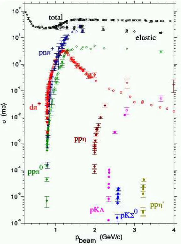
ex-periments on internal and external targets. . . 10 2.2 Cross sections for pp interactions as a function of the beam momentum (data

from CELSIUS, COSY, IUCF, SATURNE). Figure is taken from [26] . . . . 12 2.3 The COSY-TOF Detector. The beam enters from left, passes through the

small cryotarget and the evacuated tank. Start detector and tracker are close to the target. The big stop detector hodoscopes cover the inner surface of the vacuum tank. . . 14 2.4 The target system. The cold parts below the flange are in vacuum. The

necessary super isolation is removed in the picture. . . 16 2.5 Schematic view of the actual start detector and tracking system (Erlanger

start detector). . . 18 2.6 A sketch of the TOF spectrometer shows the Quirl, the Ring and one of the

barrels . . . 19 2.7 Schematic view of the Quirl detector showing the three layers. The elements

which are hit by two particles are indicated in black . . . 20 3.1 Two hodoscope planes can fake two possible Λ decay vertices due to insufficient

information. . . 22 3.2 Construction elements for a single straw tube: aluminized Mylar tube, 1cm∅

end caps with gas tubes, counting wire going through all elements and crimp pins which are finally glued into the 3 mm∅ extensions which are used for transversal fixation. . . 24 3.3 End structure of the straw double plane. The springs provide cathode

con-tacting. The crimp pins make contact to the conducting wires. The straws are fixed transversally by positioning the 3mm∅ cylindrical extensions of the end-caps in corresponding holes in a > 1m long belt. The conductive belt is removed. . . 25 3.4 Three straw frames mounted in steps of 120o _{around the beam direction. One}

also sees the central aperture for beam passage. . . 26 VII

(10)

VIII LIST OF FIGURES

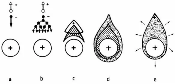
3.5 Time development of an avalanche in the Straw tube . . . 27 3.6 Time difference between creation of movable charges in the gas on the

par-ticle track and appearance of an avalanche signal on the counting wire. The coordinate information from a single straw is a ”cylinder of closest approach” [62]. . . 28 3.7 Ionization energy loss rate in various materials. The figure is taken from [73] 29 3.8 Cross sections for electron collisions in Ar. The figure is taken from [71] . . 31 3.9 Cross sections for electron collisions in CO2. The figure is taken from [71] . 32

4.1 Time development of the pulse in the straw tube. The pulse shape obtained with several differentiation time constants is also shown. Figure is taken from [63] . . . 35 4.2 Picture of the ASD-8 chip (upper left), ASD-8 input board (upper right) and

ECL converter (lower) . . . 36 4.3 Wiring diagram of the preamplifier . . . 37 4.4 Analog signal (from the cosmic particle) after preamplifier and digitized form

it behind the ECL converter. Two electron clusters appear in the event shown. 38 4.5 Simulated frequency response of the preamplifier [83]. Input signal -40 dB. . 39 4.6 Schematic of the ASD-8 input board . . . 39 4.7 The schematic of the ASD-8 input board. R1 and R2 are selected such that

75 ohm impedance matching is fulfilled . . . 40 4.8 The ASD-8 threshold vs minimum signal amplitude . . . 41 4.9 Left picture is the simulation of the input board with 4.7pF capacitor. The

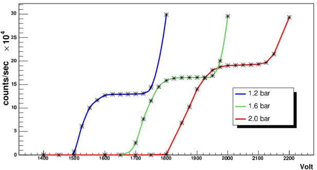
signal shape of the straw output remains nearly unchanged. Right is the simulation of the input board with 1pF capacitor. Triangle signal is given to the board as an input signal. . . 42 5.1 measured wire tension/g of 448 straws . . . 44 5.2 The relationship between HV and count rate with a 5.9keV γ source (F e55_{) for}

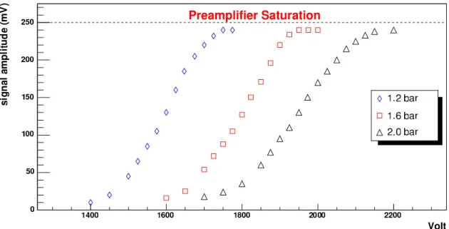
three different pressures . . . 45 5.3 HV vs signal amplitude for three different absolute pressures of 1.2, 1.6, 2bar. . . 46 5.4 Two crossed straw frames placed behind the TOF for the performance test with

the beam. Directly at the exit of the TOF tank one can see the quadratic frame of the 4mmthick fiber hodoscope which creates straggling. . . 47 5.5 Yellow and blue: straw analog signals from the deuteron beam from COSY, pink:

digital output derived from the blue signals. (Green is not used) . . . 48 5.6 Beam profile measured with one plane with 15 straw tubes. Channel 12 was

defect. . . 48 5.7 Signal amplitude fromF e55_{source versus distance along the wire for two straw}

tubes at 2040 V and 1950V. The plot a) corresponds to a straw irradiated locally with upto 1011_{deuterons per cm counting wire. b) shows a straw which}

was not strongly irradiated. The zero point is the preamplifier side of the tube. 50 5.8 Averaged signals of the illuminated straw tube from Fig.5.7 at the distances

of ≈50cm (small signal from degraded region) and ≈ 45cm (big signal from good counting region). . . 51

(11)

LIST OF FIGURES IX

5.9 Microscope picture of the irradiated region on the 20µ∅gold plated tungsten count-ing wire. Horizontal and vertical lengths of the picture are 0.77mm and 1.12mm

respectively. . . 52 5.10 Microscope picture of the same wire as in Fig.5.9 in an unirradiated region.

Hori-zontal and vertical lengths of the picture are 0.77mmand 1.12mmrespectively. . 53 5.11 Irradiated region of the aluminized Mylar (magnification lower by a factor 8 with

respect to Fig.5.9 and Fig.5.10). Clear traces of aging effect are seen on the alu-minum surface as cloudy strips precisely orthogonal to the wire direction. The underlying pattern of inclined fine strips is a property of the aluminum mirror on the (undisturbed) Mylar surface. Horizontal and vertical lengths of the picture are 6.17mmand 8.95mmrespectively. . . 54 5.12 Same irradiated region on the cathode as in Fig.5.11 scaled up 8 times (same

mag-nification as in Fig.5.9 and Fig.5.10). The black regions are undisturbed, shiny aluminum mirror surface. The cloudy white strips are 50µmto 300µmwide and up tocm long. There the mirror surface is damaged. Horizontal and vertical lengths of the picture are 0.77mm and 1.12mm respectively.. . . 55 5.13 Region of the aluminized Mylar which was not irradiated. No cloudy strips are

seen. The upward going line is the counting wire. This pattern can be directly compared to Fig.5.11 which has the same scale and orientation with respect to the counting wire. Horizontal and vertical lengths of the picture are 6.17mm and 8.95mmrespectively. . . 56 5.14 χ2_{-distribution and isochrone residuals ∆}_r

i of all reconstructed tracks. Mean

and deviation (σ) of the residuals Gauss-fit are 4µm and 83µm respectively. Figure is taken from [93] . . . 58 5.15 Spatial resolution of the straw tube. . . 59 5.16 Efficiency vs tube radius . . . 59 6.1 Geometrical impulse reconstruction from the vectorial sum of two outgoing

directions to the beam momentum vector. . . 62 6.2 χ2_{-value distribution for the reaction} _pp_→ _dπ+_{. The first peak corresponds}

topp→dπ+ _{events. Figure is taken from [95] . . . .} ₆₃

6.3 Collection of the world data on total cross section for the reactionpp→dπ+_.

The red points are the result of the Dr. Wissermann’s analysis (σtot = 46.6

at 2950MeV /c and σtot = 31.5 at 3200MeV /c). Figure is taken from [95]. . . 64

6.4 Angular distribution for pp→dπ+_{. Figure is taken from [95]. . . .} ₆₅

6.5 The longitudinal and transversal momentum components as obtained from the experimental data, using the actual TOF setup without straw tracker. Geometry and time of flight informations were used at the event reconstruc-tion. . . 67 6.6 The longitudinal and transversal momentum components from the simulation

data, with the straw tracker replacing the fiber hodoscopes. Only geometry information was used. Both resolution and acceptance are improved . . . . 67 6.7 Missing mass spectra for the reaction pp → dπ+ _{from experimental data of}

(12)

X LIST OF FIGURES

6.8 Missing mass spectra for the reaction pp → dπ+ _{from simulation data with}

Straw tracker. . . 69

7.1 The cosmic ray test facility. Two orthogonal hodoscopes made from 90o _crossed straw tube double planes are sandwiched between the two plastic scintillators which provide a trigger coincidence.. . . 72

7.2 Schematic side view of the cosmic ray test facility with distances as it was used for the tests. . . 72

7.3 The electronic setup used in the measurements. . . 73

7.4 The DAQ Process. . . 74

7.5 Measured drift times from 4 different straw tubes. x-axis is drift time (nsec) and y-axis is the counts. . . 75

7.6 R(t) curves for the 4 straws from Fig.7.5 with 2bar absolute pressure and 2040V high voltage. . . 76

7.7 χ2 _{histogram for 8 responses tracks} _{. . . .} ₇₇

7.8 Fitted plane in which track (blue line) lies together with straw tubes (black circles) and the cylinders (red circles) in 2 dimension (YZ-plane projection along x axis). Straw numbers (str 1,2,3,4) increase from bottom to top. . . 78

7.9 Distribution of firing straws out of 8 straw responses (one per plane at most) in the test facility. The corrected ratio (8 responses/7 responses) under geometry consideration amounts to ≈95. . . 79

7.10 Dependence of firing number of straws out of 8 planes as function of a common single straw efficiency ². . . 80

7.11 Response multiplicity of the 4 double planes. 1. and 2. double planes are orthogonal and 3. 4. planes parallel to the trigger scintillators. . . 81

7.12 Simulated cosmic hit distribution between the two trigger scintillators. Close to the scintillators the hit distribution is uniform. Between the scintillators the hit distribution peaks in the center. . . 82

7.13 Illumination distribution of cosmic tracks on the circular test scintillator plane. 8 and only 8 fired straws from 8 planes are required. The observed density fluctuations come from a folding of different straw efficiencies. A χ2 _<_{5 (Fig.7.7) cut on track} fitting is applied. . . 83

7.14 QDC (left) and TDC (right) values of the circular test scintillator. . . 84

7.15 Geometry of the circular test scintillator with some few Cherenkov light responses from the plexi light guide. . . 84

7.16 Left: hit points of the all cosmic tracks (same as in Fig.7.13) on the test scintillator’s plane. Right: hit distribution with the test scintillator response as veto. . . 85

7.17 Illumination distribution of cosmic tracks on the square test scintillator. . . 86

7.18 QDC (left) and TDC (right) values of the square test scintillator. . . 86

7.19 Geometry of test scintillators, after χ2_cut_. _{. . . .} ₈₇

7.20 Left: hit points of the all cosmic tracks on the square test scintillator’s plane (same as in Fig.7.17). Right: hit distribution with the test scintillator response as veto. . 87

7.21 QDC values for light output of the circular test scintillator along the axis of light guide a) and along the transversal axis b). . . 88

(13)

LIST OF FIGURES XI

7.22 Quasi focal point in a circular scintillator which gives about parallel reflected light from the cylindrical boundary [14]. This focusing disappears when the light is emitted from points closer to the light guide (left). . . 89 7.23 QDC values of the square test scintillator along the axis of light guide a) and along

the transversal axis b). . . 89 7.24 Left geometry of the plastic light guide, right QDC values from the light guide. . 90 7.25 Superposition of the QDC spectra from scintillator and light guide. . . 91 7.26 Left: hit distribution of the cosmic ray on the wire plane. Right: same distribution

with test straw as veto. . . 91 7.27 Reconstructed geometry of the straw tube.. . . 92 7.28 A few radial distance circles calculated from the R(t) calibration curve are drawn

around the track positions. The wire position appears as tangent to the distance circles. . . 93 7.29 The full set of distance circles together with the resulting tangent which

approxi-mates the wire position. . . 94 7.30 The expected radius determined from wire position and hit points on horizontal

axis and radius determined from straw timing andR(t) calibration on vertical axis. 95 7.31 r_R₍_t₎_calib - rhit points. . . 96

7.32 TDC resolution histogram. Obtained with pulser signals at two different time. . . 96 A.1 Each container class represent a sub-detector of COSY-TOF. Information of

each triggered channel is stored as a hit-class . . . 100 A.2 Conversion of detector data from tape using four intermediate data formats

(RAW, LST, CALtemp, CAL). The CAL-format is fully calibrated and the basis of all data analysis. . . 101 B.1 The TDC spectrum of the wound layers of the Quirl detector before (left) and

after (right) calibration. TDC values in units of 100 psec. Figure is taken from [55]. . . 106 B.2 The ADC spectrum of the wound layers of the Quirl detector before (left) and

after (right) calibration. Figure is taken from [55]. . . 108 C.1 P8(k) versus². . . 110

(14)

(15)

List of Tables

1.1 Quarks with their charges and masses. . . 1 1.2 Some baryons and mesons together with their quark contents, electric charges,

masses, life times and decay modes. . . 2 3.1 Circular acceptances of the first and second Fiber Hodoscopes (at their

posi-tion in the TOF) and straw tracker planes at the same posiposi-tions. . . 23 3.2 Anode wire and Cathode tube properties . . . 25 3.3 Some properties of different gases. Z and A are charge and atomic weight.

EX,Ei excitation and ionization energy respectively,Wi is the average energy

required to produce one electron-ion pair in the gas,dE/dx is the most prob-able energy loss by a minimum ionizing particle,X0 is the radiation length. 29

3.4 Experimental parameters for different gases. . . 34 4.1 Four configurations for the input board. . . 41 A.1 The most important TofRoot classes . . . 99

(16)

Chapter 1 Introduction

1.1 Motivation

High energy physics deals basically with the study of the ultimate constituents of matter and nature of the interactions between them. Experimental research in this field of science is carried out with particle accelerators and their associated detection equipment. High energies are necessary for two reasons; first, in order to localize the investigations to very small scales of distance associated with the elementary constituents, secondly many of the fundamental constituents have large masses and require correspondingly high energies for creation and study.

Nearly seventy years ago, only a few elementary particles the proton, neutron, the elec-tron and neutrino, together with the electromagnetic field quantum photon were known. The universe as we know it today appears indeed to be composed almost entirely of these particles. However, attempts to understand the details of the nuclear force between protons and neutrons, as well as to follow up the pioneering discoveries of new, unstable particles observed in the cosmic rays, led to the construction of ever larger accelerators and to the observation of many new particles. These so-called ”hadrons” or strongly interacting parti-cles are unstable under terrestrial conditions but are otherwise just as fundamental as the familiar proton and neutron [1]. Our present model of the constituents of matter is that they consist of fundamental point like spin 1/2 fermions the quarks [2], with fractional electric charges and theleptons, like the electron and neutrino, carrying integral charges.

The known quarks are listed in Table-1.1 ([3]). Quarks are always confined in compound Quark Electric charge (e) Mass

u (Up) 2/3 2-8 MeV d (Down) -1/3 5-15 MeV c (Charmed) 2/3 1-1.6 GeV s (Strange) -1/3 100-300 MeV t (Top) 2/3 168-192 GeV b (Bottom) -1/3 4.1-4.5 GeV Table 1.1: Quarks with their charges and masses.

(17)

2 Introduction

systems which extend over distances of about 1f m. The most elementary quark systems are baryons which have net quark number three, and mesons which have net quark number zero. In Table-1.2 some baryons and mesons together with their quark contents, electric charges, masses, life times and decay modes are listed (the values are taken from [4]).

Particle Quark content Electric charge (e) Mass (MeV) cτ Decay Mode

p uud 1 938.27 n ddu 0 939.56 2.65∗108_{km pe}−_ν_¯ e pπ0₍₅₁_._6%) Σ+ _uus ₁ _1189.37 _{2.4 cm} _nπ+₍₄₈_._3%) Σ0 _uds ₀ _1192.64 ₂_.₂_∗₁₀−11_m _Λ_γ Σ− _dds _-1 _1197.45 ₄_.₄_cm _nπ−₍₉₉_._8%) pπ−₍₆₃_._9%) Λ uds 0 1115.68 7.89cm nπ0₍₃₅_._8%) π+ _u¯d ₁ _139.57 ₇_.₈₀_cm _µ+_ν µ(99.99%) π− _d¯u _-1 _139.57 ₇_.₈₀_cm _µ+_ν µ(99.99%) 2γ(98.8%) π0 _(u¯u+d¯d)/√₂ ₀ _134.97 ₂₅_nm _e+_e−_γ₍₁_._2%) µ+_ν µ(63.5%) K+ _u¯s ₁ _493.68 ₃_.₇₁_m _π+_π0₍₂₁_._2%) µ+_ν µ(63.5%) K− _s¯u _-1 _493.68 ₃_.₇₁_m _π+_π0₍₂₁_._2%)

Table 1.2: Some baryons and mesons together with their quark contents, electric charges, masses, life times and decay modes.

Quantum Chromodynamics (QCD) is considered to be the underlying theory of the strong interaction, with quarks and gluons as fundamental degrees of freedom.

QCD is simple and well understood at short-distance scales, much shorter than the size of a nucleon (<10−15_{m) [5]. In this regime, the basic quark-gluon interaction is sufficiently}

weak. Here, perturbation theory can be applied, a calculation technique of high predictive power yielding accurate results when the coupling strength is small. In fact, many pro-cesses at high energies can quantitatively be described by perturbative QCD within this approximation.

The perturbative approach fails when the distance among quarks becomes comparable to the size of the nucleon, the characteristic dimension of our microscopic world. Under these conditions, the force among the quarks becomes so strong that they cannot be further separated. This unusual behavior is related to the self-interaction of gluons: gluons do not only interact with quarks but also with each other, leading to the formation of gluonic flux

(18)

1.2 Scattering Experiments 3

tubes connecting the quarks [6]. As a consequence, quarks have never been observed as free particles and are confined within hadrons, complex particles made of 3 quarks (baryons) or a quark-antiquark pair (mesons). Baryons and mesons are the relevant degrees of freedom in our environment.

In the domain of low energies and momentum transfers (q2 _∼₁₋₅_GeV2_{, medium-energy}

physics) analytical QCD calculations are not reliable. In this domain, the useful methods are: the chiral effective theory, lattice calculations and meson exchange models [7]. In these theories, the properties of nuclei and nuclear reactions are described in terms of nucleons and mesons, interacting on a scale of 1 fm or larger. The nucleon-nucleon interaction at these distances is described by potentials derived from meson exchange models and adjusted to experimental data. The distance of interaction is governed by the mass of the meson. Light pions (π0,+,−_{) mediate the long- and medium-distance interactions (}_> ₀_.₇_{f m, attractive}_);

heavy mesons (ω, ρ) are responsible for a strong short-range force (repulsive) [8].

The physics program at the medium energy hadron accelerators (TRIUMF, LAMPF, PSI, LEAR, SATURNE, IUCF, CELSIUS and COSY) was and is focusing on studies of the production and the decay of light mesons and baryon resonances and the conservation or violation of symmetries [9].

Investigations of the production of mesons and their interactions with nucleons are based on measurements determining the total and differential production cross sections and their dependence on the energy of the interacting nucleons. When one wants to study excited hadrons then the detector has to measure their stable decay products. This means that in the exit there are normally more than two outgoing particles. To establish a comprehensive description of the medium-energy physics, high quality measurements are needed, for which two very important requirements have to be fulfilled:

• a high acceptance detector system • a beam of high quality and intensity

1.2 Scattering Experiments

Much of what we know about nuclei and elementary particles, the forces and interactions in atoms and nuclei has been learned from scattering experiments, in which atoms in a target bombarded with beams of particles [10]. The earliest were the alpha-particle scattering experiments of Ernest Rutherford. In 1906, to probe the structure of the atom, Rutherford observed the deflection of alpha particles as they pass through bulk matter (a thin sheet of gold foil). He observed that alpha particles from radioactive decays occasionally scatter at angles greater than 90o_{, which is physically impossible unless they are scattering off}

something more massive than themselves. This led Rutherford to deduce that the positive charge in an atom is concentrated into a small compact nucleus [11]. Thus, nucleons scattered from atoms at various scattering angles reveal information about the nuclear forces as well as about the structure of nuclei.

The important observables to extract the physics from the scattering experiments are e.g. the energy dependent total cross section σ(²) and the differential cross section dσ/dcos(θ) depending on the angular correlation between entrance and exit directions. Observables

(19)

4 Introduction

are always of the type: number of events per some phase space interval and per number of beam particles. The cross section shows resonance massesMR and widths ΓR. The angular

distributiondσ/dcos(θ) depends on the square of the wave function and contains information on spin, parity and angular momentum content of the reaction. Excited hadrons appear as peaks in subsystem mass spectra.

In Fig.1.1 a typical scattering experiment illustrated. A stream of particles, all at the same direction and energy, moves through the target (very small spot) where some of the particles interact. The reaction particles are measured by a detector. The scatterer is

Figure 1.1: Principle of a scattering experiment on an external target. The beam passes through a cell with thin windows, which contains the target material. Reaction products are measured by surroundings detectors which cover the full solid angle in ideal case.

represented by an area σ called cross section. It is the measure of the probability that a scattering can happen. The available beam intensity (n= number of particles per second) and the target thickness (density ·length· NA(Avogadro number) = target particles per

unit area) define the luminosity L(reaction s−1_cm2_{) which is:}

L=n·ρ·d·NA

The total reaction rate is given by:

Rate=L·σ

where σ is the cross section of the reaction or interaction probability between particles of the beam and target. The unit of σ is barn (1mb = 10−27_cm2_{). With a 4}_mm _{thick liquid}

hydrogen target having the thickness of 1.7∗1022_protons/cm2 _{and a proton beam of 10}9_s−1_,

the luminosity is:

(20)

1.2 Scattering Experiments 5

With σpp = 40mb= 4∗10−26cm2, the reaction rate in the target is 6.8∗105s−1. In order to

measure the differential cross section, the following informations are needed [12]: • intensity of the beam,

• total measurement time,

• solid angle coverage of the detector, • scattering angle,

• number of particles scattered into this solid angle, • thickness of the target,

• density of the target,

• atomic weight of the target material, • Avagadro number (NA= 6.022∗1023)

In general a detector covers only a certain part of the solid angle. One measures the differential cross section defined as:

dσ(θ, φ)

dΩ(θ, φ) =

number of particle scattered in to the dΩ

j (current density of the beam) and tries to extrapolate the full angular range.

If we consider the scattering of particles on a potential V(r) which is only nonzero at |r|< a, the scattering process is described in the non-relativistic quantum mechanics by the sum of an incoming plane wave and an outgoing spherical wave [12]:

ΨT(~(r) = A

"

ei~k~r₊_f₍_{θ, φ}₎eikr

r

#

where f(θ, φ) is the scattering amplitude. The density of the particles is given in quantum mechanics by P = Ψ∗_{Ψ. For incoming particles with the velocity of} _v

in, the current density

is jin =vinP =A2vin. Similarly for the outgoing particles the current density is

jout =vout|Ψ|2 =vout|f(θ, φ)|2A2/r2. Using the current densities one can write the differential

cross section in terms of scattering amplitude [12]:

dσ(θ, φ) dΩ(θ, φ) =|f(θ, φ)| 2 f(θ, φ) is: f(θ, φ) = −2πm h2 Z ei~k~r0 V(r0_)Ψ T(~r0)d3r0 (1.1)

(21)

6 Introduction

1.3 Event Reconstruction and

Feasibility of an Experiment

The detector volume is filled with devices which the particle traverse and in which they leave pieces of information by creating light flashes or movable electric charges (excitation and ionization). The event record of an experiment consists of signals from all particles of an interaction. After sorting out which informations are related to the same particle the kinematical properties of each particle have to be reconstructed to reveal the physical nature of the whole event [13].

In ideal case a detector must

• measure over the complete possible kinematical region for the desired reaction (100 % acceptance)

• make it possible to determine the four vectors (E, ~p) of all reaction particles (kinemat-ical completeness)

For kinematically complete events in which all four vectors are known (both in entrance and exit), all possible physical observables can be determined, but the precision which an experiment can reach is limited by

• precision in the kinematical coordinates (four vector components) • statistical accuracy (number of events per interval)

• amount of background

• efficiency with which the detector and reconstruction procedure cover the phase space of the reaction

The precision in the determination of the four vector of a charged particle depends on the accuracies in the track direction, absolute momentum and identification of the particle mass. Except for the mass, these kinematical quantities can be measured by means of high granularity but approximately massless geometry detectors when particles are charged.

If the detector provides more information than necessary (over constraints) one can and should use the additional information to improve the precision in the event reconstruction by a fit procedure.

If we assume a reaction in which the beam and target particle go into several exit particles 1 + 2 +· · ·, then we can write for that an equation for the four vectors P:

Pbeam+Ptarget = P1+P2· · ·

In explicit four vector notation, this describes simply four equations for the simultaneous energy and momentum conservation and writes:

     E px py pz      beam +      E px py pz      target =      E px py pz      1 +      E px py pz      2 +· · · (1.2)

(22)

1.3 Event Reconstruction and

Feasibility of an Experiment 7

There holds the relativistic relation between energy and momentum E2

i =m2i +p~i2

where ~p = (px, py, pz) =|~p|(nx, ny, nz)~n is the unit vector of direction cosines (|~n|= 1 and

n2

x+n2y +n2z = 1).

In Eq.1.3 an equivalent information to the four vectors (in Eq.1.2) is written.

¯ ¯ ¯ ¯ ¯ ¯ ¯ ¯ ¯ mb nbx nby ±|pb| ¯ ¯ ¯ ¯ ¯ ¯ ¯ ¯ ¯ ⊕ ¯ ¯ ¯ ¯ ¯ ¯ ¯ ¯ ¯ mt ntx nty ±|pt| ¯ ¯ ¯ ¯ ¯ ¯ ¯ ¯ ¯ → ¯ ¯ ¯ ¯ ¯ ¯ ¯ ¯ ¯ m1 n1x n1y ±|p1| ¯ ¯ ¯ ¯ ¯ ¯ ¯ ¯ ¯ ⊕ ¯ ¯ ¯ ¯ ¯ ¯ ¯ ¯ ¯ m2 n2x n2y ±|p2| ¯ ¯ ¯ ¯ ¯ ¯ ¯ ¯ ¯ (1.3)

The directional unit vectors~n are worth only two variables, sincen2

z = 1−n2x+n2y. The

sign ofnzis kept in the momentum±|p|and distinguishes forward or backward going tracks.

This table allows to count over constraints and thus judge if a given experimental setup provides enough information for a kinematically complete event construction [14].

For example, if we assume a pure geometry detector, for the reaction pp → dπ+ _(no

velocity measurement for d and π+_{), we have:}

m→ nx → ny → |p| → ¯ ¯ ¯ ¯ ¯ ¯ ¯ ¯ ¯ ¯ ¯ ¯ ¯ ¯ p √ √ √ √ ¯ ¯ ¯ ¯ ¯ ¯ ¯ ¯ ¯ ¯ ¯ ¯ ¯ ¯ ⊕ ¯ ¯ ¯ ¯ ¯ ¯ ¯ ¯ ¯ ¯ ¯ ¯ ¯ ¯ p √ √ √ √ ¯ ¯ ¯ ¯ ¯ ¯ ¯ ¯ ¯ ¯ ¯ ¯ ¯ ¯ → ¯ ¯ ¯ ¯ ¯ ¯ ¯ ¯ ¯ ¯ ¯ ¯ ¯ ¯ d √ √ √ 0 ¯ ¯ ¯ ¯ ¯ ¯ ¯ ¯ ¯ ¯ ¯ ¯ ¯ ¯ ⊕ ¯ ¯ ¯ ¯ ¯ ¯ ¯ ¯ ¯ ¯ ¯ ¯ ¯ ¯ π+ √ √ √ 0 ¯ ¯ ¯ ¯ ¯ ¯ ¯ ¯ ¯ ¯ ¯ ¯ ¯ ¯

2 overconstraints

where√ means information produced by detector and 0 no information produced. We have two unknown momenta but four equations from the momentum conservation so we have already two over constraints.

With a time of flight information, givingβ~ and in turn ~p, (together with a mass assump-tion ~p = m·β~ ·γ) we have except the masses no unmeasured information and four over constraints in this case.

¯ ¯ ¯ ¯ ¯ ¯ ¯ ¯ ¯ ¯ ¯ ¯ ¯ ¯ p √ √ √ √ ¯ ¯ ¯ ¯ ¯ ¯ ¯ ¯ ¯ ¯ ¯ ¯ ¯ ¯ ⊕ ¯ ¯ ¯ ¯ ¯ ¯ ¯ ¯ ¯ ¯ ¯ ¯ ¯ ¯ p √ √ √ √ ¯ ¯ ¯ ¯ ¯ ¯ ¯ ¯ ¯ ¯ ¯ ¯ ¯ ¯ → ¯ ¯ ¯ ¯ ¯ ¯ ¯ ¯ ¯ ¯ ¯ ¯ ¯ ¯ d √ √ √ √ ¯ ¯ ¯ ¯ ¯ ¯ ¯ ¯ ¯ ¯ ¯ ¯ ¯ ¯ ⊕ ¯ ¯ ¯ ¯ ¯ ¯ ¯ ¯ ¯ ¯ ¯ ¯ ¯ ¯ π+ √ √ √ √ ¯ ¯ ¯ ¯ ¯ ¯ ¯ ¯ ¯ ¯ ¯ ¯ ¯ ¯

4 overconstraints

An example of three outgoing particles with a charged particle detector (like TOF) is

pbeam+ptarget →p+p+π0 (or γ, or ”nothing”)

(23)

8 Introduction informations). ¯ ¯ ¯ ¯ ¯ ¯ ¯ ¯ ¯ ¯ ¯ ¯ ¯ ¯ p √ √ √ √ ¯ ¯ ¯ ¯ ¯ ¯ ¯ ¯ ¯ ¯ ¯ ¯ ¯ ¯ ⊕ ¯ ¯ ¯ ¯ ¯ ¯ ¯ ¯ ¯ ¯ ¯ ¯ ¯ ¯ p √ √ √ √ ¯ ¯ ¯ ¯ ¯ ¯ ¯ ¯ ¯ ¯ ¯ ¯ ¯ ¯ → ¯ ¯ ¯ ¯ ¯ ¯ ¯ ¯ ¯ ¯ ¯ ¯ ¯ ¯ p √ √ √ √ ¯ ¯ ¯ ¯ ¯ ¯ ¯ ¯ ¯ ¯ ¯ ¯ ¯ ¯ ⊕ ¯ ¯ ¯ ¯ ¯ ¯ ¯ ¯ ¯ ¯ ¯ ¯ ¯ ¯ p √ √ √ √ ¯ ¯ ¯ ¯ ¯ ¯ ¯ ¯ ¯ ¯ ¯ ¯ ¯ ¯ ⊕ ¯ ¯ ¯ ¯ ¯ ¯ ¯ ¯ ¯ ¯ ¯ ¯ ¯ ¯ π0 ₍_γ₎ √ 0 0 0 ¯ ¯ ¯ ¯ ¯ ¯ ¯ ¯ ¯ ¯ ¯ ¯ ¯ ¯

1 overconstraint

In this case, we have three unknowns (momentum of the neutral particle) and 1 over con-straint.

At low energy close to the π0 _{threshold and with a time of flight information for the}

two protons three different hypothesis for the neutral particle are possible, pion, photon or nothing. This reaction pp → ppX0 _{was published by TOF [15]. A detector, having}

good enough resolution, allows to evaluate all three channels since the over constraint gives selectivity.

(24)

Chapter 2 Experimental System

2.1 COSY Accelerator

COSY is a cooler synchrotron and storage ring depicted in Fig.2.1. It delivers very high precision polarized and unpolarized beams of upto ≈ 2∗1011 _{protons and deuterons per}

machine cycle in the momentum range from 300MeV /cto 3600MeV /c[16, 17]. This goal is accomplished by using an electron cooling system and a stochastic cooling system.

The electron cooler of COSY is designed for electron energies up to 100keV, thus to cool protons up to a momentum of 600MeV /c [18, 19]. An electron beam guided in parallel to the protons (deuterons) reduces; the transversal and longitudinal momentum by friction and makes phase-space-dense ion beams before acceleration to a requested energy [20]. Electron cooling is used after stripping injection of H− _or _D− _{ions. With the stochastic cooling}

covering the range from 1.5GeV /c up to maximum momentum, deviations from the beam are determined for sub samples of the beam and then in each turn a correction on the samples is applied. From turn to turn new samples are prepared by mixing [21, 22].

The beam preparation needs 2 to 12sec (acceleration upto 2sec, electron cooling upto 10sec). The spill out time can be stretched from few seconds to minutes by stochastic extraction. On internal targets operation times can be upto hours for one cycle if stochastic cooling compensates the beam blow up by the target.

The COSY consists of two sources for unpolarized H−_/D− _{- ions and one for polarized}

H− _-/ _D−_{- ions, the injector cyclotron JULIC that accelerates the} _H− _{- ions up 300}_{MeV /c}

andD− _{- ions up 600}_{MeV /c}_{, the cooler ring COSY with a circumference of 184 m delivering}

protons up desired momentum [16, 23]. Injection into COSY takes place via charge exchange of theH−_{- or}_D−_{- ions over 20}_ms_{with a linearly decreasing closed orbit bump at the position}

of the stripper foil. The polarized source presently delivers 8.5µA of polarized H− _{- ions}

[23].

Four internal target areas (ANKE, COSY-11, COSY-13, EDDA) are available for experi-ments with a circulating beam. The beam can also be extracted via the stochastic extraction mechanism and is guided to three external experiment areas (magnetic spectrometer BIG KARL, Time Of Flight spectrometer TOF and JESSICA). The emittance of the extracted cooled beam is only ²= 0.4π mm mrad [24].

(25)

10 Experimental System

Figure 2.1: The COSY accelerator at the research center J¨ulich and the positions of ex-periments on internal and external targets.

(26)

2.1 COSY Accelerator 11

2.1.1 Physics in COSY

The COSY accelerator with the energy range and beam quality that it provides, makes it possible to study the structure of mesons and baryons in the confinement regime of QCD. This field includes the analysis of decay properties of mesons and baryon excitations and interactions of meson meson, meson baryon and baryon baryon systems. The experimental studies are characterized by keywords like threshold measurements (it is possible due to the high quality of beam and target. Beam diameters at targets are available with divergencies below 1mrad.), strangeness production, final state interaction, medium modification and reaction mechanisms [25].

Threshold measurements are instructive for the interpretation of elementary interactions. The relative velocities of the ejectiles are low which favors s-waves and final state interac-tions. At threshold the momentum transfer is high since incoming particles have high and the outgoing particles have small center of mass momenta. The transfer is practically the center of mass momentum of the input channel. This large momentum transfer and s-wave dominance at threshold enhance heavy meson exchanges [26].

The strangeness production is an excellent tool to study hadron dynamics [27]. Due to the high selectivity for the detection of delayed decays of hyperons andKsmesons it is

exper-imentally particularly precise. Questions concerning the strangeness content of the nucleons and the reaction mechanisms for the dissociation can be addressed by such studies. For the

pp→pK+_{Λ [28] reaction it is comparatively easy and precise to measure the Λ polarization}

via the asymmetry of the parity violating weak decay Λ → pπ−_{. In a simple quark model}

this is related to the s-quark polarization. With a polarized beam and polarized target a detailed analysis of the spin degrees of freedom can be done in Λ production reactions.

Modifications of the properties and interactions of hadrons within the nuclear medium are another interesting field. Questions here are for example the lifetime of hyper nuclei, specific reaction mechanisms and possible medium effects especially on K-mesons which may be isolated in subthreshold production experiments [29].

With COSY a wealth of experimental data has been accumulated during the last decade, which differ to previous measurements with respect to the quality and the amount of the data. Fig.2.2 gives an overview of the world data (including COSY) on total cross sections in pp interactions below 4GeV /c beam momentum.

(27)

Figure 2.2: Cross sections for pp interactions as a function of the beam momentum (data from CELSIUS, COSY, IUCF, SATURNE). Figure is taken from [26]

(28)

2.2 COSY-TOF Detector System 13

2.2 COSY-TOF Detector System

Highly sophisticated detector systems are in operation either at the internal COSY beam or located at extracted beams in external areas. The time-of-flight spectrometer TOF is one of the main experimental facilities at the external beam lines of the COSY.

The investigations at COSY-TOF [30] concentrate mainly on the light and medium mass meson production, proton-proton bremsstrahlung and associated strangeness meson-baryon production by measuring following reactions

• pp→pK+_Λ_{, pK}+_Σ0_{, pK}0

sΣ+ [28, 31, 32, 33]

• pp→pp, ppγ, ppπ0_{, ppη, ppη}0 _{[15, 34, 35, 36, 37, 38]}

• pp→pnπ+_{, dπ}+_{, ppπ}+_π−_{, ppω} _{[39, 40]}

• pd→3 _Heη, 3_Heη0_, 3_Heω _[41]

The COSY-TOF spectrometer is designed as a scintillator hodoscope for stable charged particles covering about 2πsolid angle in the laboratory system. The main components of the TOF spectrometer are a liquid hydrogen target, a start detector, tracker system and a system of three stop detector segments, forming a cylinder barrel with a circular endcap (Fig.2.3). The endcap consists of two concentric circular hodoscopes. Up to 3 barrel elements can be combined with the two planar front hodoscopes of 1.16 and 3 m outer diameter, providing very large solid angle coverage without holes. Fig.2.3 shows the TOF spectrometer in a 3 m long version. With two more existing barrel sections the maximal flight path in vacuum can be extended to more than 8m. Since the typical velocities of the particles in the momentum range of COSY are between approximately 25% and 99% of the speed of light [42], the flight lengths must amount to some meters in order to be able to determine the velocity sufficiently well with the available time resolution of 2.5∗10−10_sec _{(average over all detectors) [42].}

The spectrometer components are housed in a big vacuum tank [43]. So it is guaranteed that beam particles and reaction products do not undergo reactions with air, which would lead to many non-target originated events and to straggling.

A very important advantage of TOF is the absence of a vacuum tube for the beam. Such a tube would occupy space for detectors at small angles and reaction particles would have to penetrate very thick layers of this tube if they are at small forward angles. TOF detectors can be (and they are) positioned millimeters away from the passing cooled primary beam. This is particularly advantageous if one is going to detect Λ→ pπ+ _or _K

s →π−π+ decays

which have decay vertices close to the beam in the few cm distance from the target. TOF is unbeatable best suited for reaction studies with Λ and Ks.

In order to calibrate the time measurement, the start and stop scintillators are connected to a nitrogen laser UV light calibration system by quartz light guides.

(29)

Figure 2.3: The COSY-TOF Detector. The beam enters from left, passes through the small cryotarget and the evacuated tank. Start detector and tracker are close to the target. The big stop detector hodoscopes cover the inner surface of the vacuum tank.

(30)

2.2.1 Target system

A very light liquid hydrogen (or deuterium) target (Fig.2.4), which is very small in order to take advantage of the excellent beam quality of COSY, has been developed and used for the external experiments at COSY [44]. Since hydrogen or deuterium are gases and have very low densities at room temperature and atmospheric pressure (0.08 g/l for H2 and 0.166 g/l

forD2), leading to reduction of the reaction probability, they are liquefied. The liquid target

with its very small amount of inactive material and thin beam windows is installed in the entrance of the TOF tank in a section with good vacuum of 10−6 ₋₁₀−7_mbar_{. The target}

construction is affected by the following requirements [45]:

• It has to stabilize the target temperature within ±0.05K in the range of liquid hydro-gen/deuterium

• The windows for the beam inlet and exit through the target cell have to be very thin but nevertheless planar

• The target thickness has to be well defined. Therefore, the target liquid should have homogenous density without any bubbles

• The time needed for large temperature changes during cooling down to the working temperature or heating up to the room temperature has to be as short as possible • The cooling system and the heat conductors have to occupy minimum space and

mini-mum solid angle. There must be minimini-mum mass in the target region in order to reduce background events and shadowing effects on reaction products before they can reach detectors

• the target should have axial symmetry

The target system used in the TOF experiments has a target cell with 6mmin diameter and normally 4mmin length. It has very thin windows of 0.9µmMylar foil. This is achieved by a stabilized pressure difference over windows of ≤ 0.2mbar in all conditions [46, 47]. The small dimensions of the target minimize the background due to double scattering and enable measurements very close to threshold. If we consider the delayed decays of strange particles occurring a few centimeters after their production in the target, the target length therefore should be much smaller than the decay length of a few centimeters to get a well defined interaction vertex. This is important for high quality kinematical reconstruction and understanding of the reactions. The very thin window foils reduce the background events from reactions on heavier nuclei in the target window foils, the energy losses and straggling of the outgoing ejectiles. With the beam from COSY of≈0.7mm∅and 4mm lH2 thickness

we obtain routinely a reaction vertex definition within < 2mm3_{. This has big advantages}

for geometrical reconstruction and background identification.

In order to keep the target in optimum conditions (constant temperature and stable density), a heat pipe-target system is developed [48, 49]. It is a closed system, which has an evaporator and condenser section where the target material acts as a working fluid which evaporates and condenses. The condenser section and evaporator section (target cell) are connected by a transport (or adiabatic) section that bridges large distances. Heat applied

(31)

to the evaporator section by an external source radiation vaporizes the working fluid. The resulting vapor pressure drives the vapor through the adiabatic section to the condenser, where the vapor condenses, releasing the latent heat of vaporization to the heat sink (cooling machine). The condensed liquid flows down to the evaporator section for re-evaporation. This gravity assisted circulation provides a stable dynamic equilibrium. The target material is liquefied by using a cooling machine. The cooling time of the system forH2/D2 from room

temperature (300K) to 15/19K is 50/45 minutes respectively [46].

Figure 2.4: The target system. The cold parts below the flange are in vacuum. The necessary super isolation is removed in the picture.

(32)

2.2.2 Start Detector

The actual start detector consists of two circular layers of 12 wedge shaped plastic scintillator sectors (δφ= 30o_{) with 1}_mm_{thickness, placed in a distance of 23}_mm_{behind the target [50].}

They deliver a reference signal for the time of flight measurement with the resolution of

σ = 170ps. In order to cover the gaps between the wedges, the two layers are rotated to each other by 15o _{leading to a} _φ _{information in steps of 15}o_{. Its outer radius is 76}_mm_{. In}

the center there is a hole of 1.4mm radius for the beam.

2.2.3 Tracker

After the start detector, there is the ”Erlanger tracker” detector (Fig.2.5), made especially to investigate the strangeness and hyperon-production [51]. Its goal is track and vertex reconstruction. It consists of a Si-µStrip detector followed by two fiber hodoscopes providing geometry informations for the tracks of charged particles.

The Si-µ Strip detector with a thickness of 520µm is 30mm far from the target. It is made of 100 concentric rings (∆r = 280µm) on one side and 128 in φ segmented elements (∆φ = 2.81o_{) on the other side. The detector has an outer radius of 31}_mm _{and a beam}

hole with a radius of 3.1mm. The 12800 pixels of the detector provide high resolution in determination of the track direction. The detector also provides energy loss information [52]. Two fiber hodoscopes complete the tracker detector system. They are made from 2× 2mm2 _{quadratic scintillating fibers, covered by cladding of about 0}_.₁_mm_{thickness. The first}

one placed 100mmdownstream from the target, consists of two layers each of 96 scintillating fibers which are rotated 90o _{relative to each other. In 2004 a new third plane is added to the}

existing system in order to increase the reconstruction efficiency. The second one is placed 200 mm far from the target and made of two times 192 fibers. It covers the active area of 1475cm2_{. Besides the energy loss of the particles, points for the primary and secondary}

tracks are provided by the fiber hodoscopes.

The straw tracker, having much higher resolution, much more depth and less mass, much larger surface will replace these fiber hodoscopes at the end of 2006. It will improve the overall performance of the experiments.

(33)

Figure 2.5: Schematic view of the actual start detector and tracking system (Erlanger start detector).

(34)

2.2.4 Stop Detector

The Quirl Ring and Barrel detectors constitute the stop detector Fig.2.6. There are no acceptance holes between these three components [53]. The barrel hodoscope consists of one layer of 96 straight scintillators which are read out from both sides [54]. It covers the large reaction angles and provides time and position information by averaging the response of the two photomultipliers at each end of the scintillator bars.

Figure 2.6: A sketch of the TOF spectrometer shows the Quirl, the Ring and one of the barrels

The central hodoscope (”quirl”) is a 3-layer (each 0.5 cm thick) scintillation counter having the inner- and outer radius of 4.2cmand 58cm. The first layer is divided into 48 wedge shaped sectors (∆φ = 7.5o_{). The second and third layers consist of 24 left- and 24 right wound}

(Archimedes) spirals. The relationship betweenφ and r isr(φ) = rmax

φmaxφwherermax = 58 cm

andφmax = 180o[52]. The overlapping area between three elements fired by a passing particle

forms a triangular pixel giving the direction of the track (Fig.2.7). This type of hodoscope was originally invented and build for measurements at the LEAR/JETSET experiments and then for CELSIUS/WASA. The advantage of the three layer geometry is also that more than one passing particle tracks can be determined unambiguously. Since all scintillator elements are symmetric under rotations around the beam axis in steps of the azimuthal angular width of an element, the Quirl detector plane is divided into equal, radially symmetric areas. Therefore, all individual scintillators in a plane are exposed to the same integral counting rate as they cover identical parts of the phase space [55]. Furthermore the hodoscope gives a fast online multiplicity and timing trigger and allows for dE/dx measurements.

The ring detector consists also of three layers of 5mm thick scintillator material. It has an inner- and outer diameter of 1.136m and 3.08m. The design is basically the same as that of the Quirl detector. The much larger surface of the ring detector is divided into 96 straight segments and 48 left- and right spirals with only 120o _{winding angle for the bent scintillators}

(35)

Figure 2.7: Schematic view of the Quirl detector showing the three layers. The elements which are hit by two particles are indicated in black

(36)

Chapter 3 New Geometry Spectrometer

”Straw Tracker” for COSY-TOF

3.1 Requirements for the Straw Tracker

The time of flight spectrometer TOF will be extended by a much better tracking system with higher resolution, much higher sampling density, and lower mass [56, 57]. Three thousand straw tubes arranged in 15 double planes will replace the existing tracking detector (fiber hodoscopes) of COSY-TOF.

The straw tracker will be placed behind the µ-strip detector and ≈ 6 cm down stream from the target. It will improve

• track resolution

• efficiency of the event reconstruction • acceptance

• transparency

in COSY-TOF experiments.

For reactions with two or three charged particles in the final state the particle momenta can be determined by measuring the direction vectors alone (see chapter 6). In this case better angular and position (track resolution) resolution directly improves the momentum resolution.

Examples of such reactions are pp→dπ+_, _pp_→_pK+_{Λ (Λ}_→ _pπ−_{). In the last reaction}

the direction of the neutral Λ hyperon can be determined by its production and decay vertex and decay plane. Both are given in first approximation by points of closest approach between thepandK tracks and the secondarypandπ−_{tracks, respectively. An intersection criterion}

on the simultaneous line fits must be imposed for the more precise final geometrical vertex determination. The momentum of a Λ can also be calculated from the decay angles of pand

π− _{with respect to the Λ track [58]. One main goal of the new track detector is to improve}

the decay vertex reconstruction, to determine all the geometrical information for pKΛ much more precisely than now.

(37)

22

New Geometry Spectrometer ”Straw Tracker” for COSY-TOF

Due to its high resolution (better than 200µm, see 5.8) and high sampling (30 planes = 30 coordinates per track), angular and position resolution will be increased significantly. This will improve the precision of all four vector components and exclude ambiguities.

If we compare θ resolution of the first fiber hodoscope with 2mmthick fibers and placed 100mm away from the target, we find ≈20mrad (arctan(2/100)), for a single straw at the same distance from the target with the worst resolution of 0.2mm, 10 times higher resolution of ≈ 2mrad is obtained. One should notice that with 30 track points the track resolution will be much better than 0.1mm in position and 0.5mrad in direction.

One of the main topics studied in the COSY-TOF experiments is hyperon production. Since the hyperons decay typically in the first 80 mm and therefore in front of the fiber hodoscopes (cτΣ+ = 24mm, cτ_Σ− = 44mm, cτ_Λ = 78.9mm), the fibers are successful in

reconstructing these decay patterns. But the weak points of these detectors is that due to the low sampling (only two space points per track) and limited resolution, there are rather frequently ambiguities from tracks crossing each other at the same detector elements which can not be solved (see Fig.3.1). The straw tracker with high sampling and much better resolution will solve such ambiguities very easily and in this way it will increase the efficiency of the event reconstruction.

target beam

ambiguous points

Figure 3.1: Two hodoscope planes can fake two possible Λ decay vertices due to insufficient information.

Moreover the straw detector will help to identify the tracks of charged π and K before they decay inside the TOF detector. The decay length L of a particle with mass m in the lab system is related to its intrinsic lifetime τ and its relativistic velocity β or to its mass and momentum p by:

L=cτ βγ =cτ p/m

For a chargedπ (K) meson with lifetime τ = 2.6∗10−8 ₍_τ _{= 1}_.₂₄_∗₁₀−8_{) we find} _cτ _{= 7}_.₈_m

(38)

3.1 Requirements for the Straw Tracker 23

(0.74m). This means, that within ≈ 6cm flight pass 1% of the π± _{mesons (8% of the} _K±

mesons) decay. If one finds such a meson track within the first 12 cm flight pass then one has a 98% (84%) chance to have the correct track direction [56]. It needs a very good tracker in order to avoid efficiency problems in reactions with several mesons.

Very important is the acceptance of a detector, its solid angle coverage. The solid angle Ω that an object covers at a point is defined as the surface area, S, of a projection of that object onto the sphere centered at that point, and can be written as Ω = S/R2 _{[59]. In}

Table-3.1 the acceptances of the first and second Fiber Hodoscopes and straw tracker at the same position are given. They are calculated from ∆Ω = 2π(1−cosθdet)/2 [14] by assuming

circular detectors, instead of squares (taking into account that overlap areas of the detector planes in different orientation can be approximated to the circle) to make the calculation easier. Therefore 20×20 cm2 ₍₄₀_×₄₀ _cm2_{) first fiber (second) hodoscope is replaced by}

circle of 20 cm (40 cm) diameter, crossing straw double planes (100×100 cm2_{) by a circle}

of 100 cm diameter, at their position in the TOF and straw tracker. The increase in the acceptance due to the straw tracker is nearly 2.8 times at the first and 2.1 times at the second fiber hodoscope’s position.

Detector/distance (from ∆Ω of

the target) inscribed circles percent of (4π) first fiber hodo./20 cm 1.84 14.6% straw tracker/20 cm 5.05 40.0% second fiber hodo./40 cm 1.84 14.6% straw tracker/40 cm 3.95 31.4%

Table 3.1: Circular acceptances of the first and second Fiber Hodoscopes (at their position in the TOF) and straw tracker planes at the same positions.

During the experiment all reaction products pass through the detectors and interact with the material of the detector by means of electromagnetic and strong interactions. This leads to straggling and secondary reactions. Massless construction (transparency) is a very important issue to avoid these unwanted effects.

The thickness of the two fiber hodoscopes is 4×2 = 8mmscintillator. A particle traverses a thickness X in radiation length (X0) ofX/X0 ≈0.019 in the fiber hodoscopes. A particle

through all 30 straw layers (the avarage Mylar thickness of 30 straw planes is < 3mm) on the other hand traverses only a thickness of X/X0 ≈ 0.013, dominated by the total Mylar

film thickness and including gas (82/18% Ar/CO2), anode wires, and aluminization of the

Mylar film. The amount of matter for a track through the passive detector end part is

X/X0 ≈0.018, including tube end plug, crimp pin, cathode belt and frame bar. Therefore,

the whole straw tracker shows the same high transparency in all directions and minimum shadowing of the following detectors in the COSY-TOF barrel [60].

The straggling angle amounts to Θstrg ∼=

q

X

Xrad(20MeV /c)/(pβ) [4], where

X

Xrad is the

thickness of the scattering medium in radiation length. Angular imperfections project back into imperfections especially in vertex positions derived from track intersections. To reduce the effect of the straggling in the vertex reconstruction, the larger the straggling the shorter the distance must be over which a back projection is made. In other words, only reducing

(39)

24

New Geometry Spectrometer ”Straw Tracker” for COSY-TOF

straggling as much as possible allows to stay with the sensitive tracker volume far enough from the target position where the track density may be easily too high.

A ”massless” construction is also needed in order to avoid secondary hadronic reactions. They could spoil the track pattern or result in shadowing effects on subsequent detector components thus cutting into the acceptance. This is a demanding criterion not only for the sensitive parts but also for the mechanical structure material, like stretching frames or mounting and adjustment devices and electronic or gas supply components. The overpressure in the straw tubes is the trick which allows to avoid heavy frame construction in the TOF straw tracker.

3.2 The J¨

ulich Straws

The straw tubes shown in Fig-3.2 consist of 1m long Mylar tubes with a diameter of 10mm

aluminized on the inner surface. The wall thickness is 30µm. Mylar is the preferred material because of its well suited mechanical properties like a high Young’s modulus and tensile strength compared with Kapton [57]. Young’s Modulus (also known as modulus of elasticity or tensile modulus) is a measure of the stiffness of a given material. Young’s modulus (measured in pascals), Y, can be calculated by dividing the tensile stress by the tensile strain [61]: Y ≡ tensile stress tensile strain = F/A0 ∆l/l0 (3.1) where F is the force applied to the object; A0 is the original cross-sectional area through

which the force is applied; ∆l is the amount by which the length of the object changes; and

l0 is the original length of the object.

The advantage of a higher Young’s modulus is the possibility to avoid large changes of the tube length under pressure and therefore to hold the wire tension nearly constant over a larger pressure range.

Lightweight plastic end-caps glued into both ends of the Mylar tube provide gas tightness. The end-caps have a 3mm diameter and 5mm long cylindrical extension with a central

Figure 3.2: Construction elements for a single straw tube: aluminized Mylar tube, 1cm∅

end caps with gas tubes, counting wire going through all elements and crimp pins which are finally glued into the 3 mm∅ extensions which are used for transversal fixation.

(40)

3.2 The J¨ulich Straws 25

stretched. These extensions are also used for a precise transversal fixation of all tubes on both ends in belts with precisely positioned holes. Gas flow is provided through thin plastic tubes which are glued into the end caps. Fig.3.3 shows the end structure of the straw tubes with crimp pins contacting the counting wires and springs providing cathode contacts between inner aluminum layer of the Mylar tubes and positioning belt. The weight of a single straw tube is <2.5g [56].

Figure 3.3: End structure of the straw double plane. The springs provide cathode con-tacting. The crimp pins make contact to the conducting wires. The straws are fixed transversally by positioning the 3mm∅ cylindrical extensions of the end-caps in corresponding holes in a >1m long belt. The conductive belt is removed.

Anode Wire W97/Re3, Au-plated (4%) ρ = 19.3g/cm3_, _σ _{= 6}_.₃_mg/L

R/L= 314Ω/m (DC-resistance) Cathode Tube Mylar film, aluminized ρ = 1.4g/cm3 _R/L _{= 40Ω}_/m

C/L≈9.8pF/m

Table 3.2: Anode wire and Cathode tube properties

The simple but new idea of this detector development is to use the anyhow existing excess pressure inside the tubes in the TOF vacuum tank to create the necessary wire tension and mechanical stability. 1bar overpressure creates on the 1cm diameter end-caps an axial force (7.85N) which is enough to make the tubes self-supporting and supply the force (0.4N) to stretch the counting wire. This means, that massive frame constructions are not necessary [57]. As thickness defining element and in order to assure correct tube positions and rectangular shape, each plane has a window like frame made of Rohacell (plastic foam density 0.05g/cm3_{) reinforced by 0}_.₃_mm_{carbon fiber compound plates. Into this frame also}