Signals: Variational Bayes Approach
Lei Yu, Jean-Pierre Barbot, Gang Zheng, Hong Sun
To cite this version:
Lei Yu, Jean-Pierre Barbot, Gang Zheng, Hong Sun. Compressive Sensing for Cluster
Struc-tured Sparse Signals: Variational Bayes Approach. 2011.
<hal-00573953>
HAL Id: hal-00573953
https://hal.archives-ouvertes.fr/hal-00573953
Submitted on 6 Mar 2011
HAL
is a multi-disciplinary open access
archive for the deposit and dissemination of
sci-entific research documents, whether they are
pub-lished or not.
The documents may come from
teaching and research institutions in France or
abroad, or from public or private research centers.
L’archive ouverte pluridisciplinaire
HAL
, est
destin´
ee au d´
epˆ
ot et `
a la diffusion de documents
scientifiques de niveau recherche, publi´
es ou non,
´
emanant des ´
etablissements d’enseignement et de
recherche fran¸cais ou ´
etrangers, des laboratoires
Compressive Sensing for Cluster Structured
Sparse Signals: Variational Bayes Approach
Lei Yu, Jean-Pierre Barbot, Gang Zheng, and Hong Sun,
Abstract
Compressive Sensing (CS) provides a new paradigm of sub-Nyquist sampling which can be considered as an alternative to Nyquist sampling theorem. In particular, providing that signals are with sparse representations in some known space (or domain), information can be perfectly preserved even with small amount of measurements captured by random projections. Besides sparsity prior of signals, the inherent structure property underline some specific signals is often exploited to enhance the reconstruction accuracy and promote the ability of recovery. In this paper, we are aiming to take into account the cluster structure property of sparse signals, of which the nonzero coefficients appear in clustered blocks. By modeling simultaneously both sparsity and cluster prior within a hierarchical statistical Bayesian framework, a nonparametric algorithm can be obtained through variational Bayes approach to recover original sparse signals. The proposed algorithm could be slightly considered as a generalization of Bayesian CS, but with a consideration on cluster property. Consequently, the performance of the proposed algorithm is at least as good as Bayesian CS, which is verified by the experimental results.
Index Terms
Compressive Sensing, Cluster Structure, Variational Bayes.
I. INTRODUCTION
Compressive Sensing (CS) is recently developed [9], [10], [15], and then attracts lots of researchers. It provides a new paradigm of sub-Nyquist sampling which can be considered as an alternative to Nyquist sampling theorem. In particular, providing that signals are with sparse representations in some known space (or domain), information can be perfectly preserved by random projection measurements.
To reconstruct the original signals, sparse prior is generally exploited into the deficient linear inverse problem, which results in lots of algorithms, Basis Pursuit (BP) [14], [8], Orthogonal Matching Pursuit (OMP) [26], CoSaMP
This work was supported by “Bourses Doctorales en Alternance”, PEPS-A2SDC of INSIS-CNRS, NSFC (No. 60872131) and FEDER through CPER 2007-2013 with INRIA Lille-Nord Europe.
L.Yu and H. Sun are with Signal Processing Laboratory, Electronic and Information School, Wuhan University, 430079, Wuhan, China. L. Yu and J-P. Barbot are with ECS-lab ENSEA, 6 Avenue du Ponceau, 95014 Cergy-Pontoise, France and EPI ALIEN, INRIA, France. G. Zheng is with INRIA Lille-Nord Europe, 40 Avenue Halley, 59650, Villeneuve d’Ascq, France.
Email address: [email protected], [email protected], [email protected], [email protected].
TABLE I
COMPARISON BETWEEN DIFFERENTCSRECOVERY ALGORITHMS.
Algorithms Is for Cluster? Num. of Clusters Size of Clusters Fixed Cluster Positions Sparsity Greedy algorithms (CoSaMP, OMP, etc) No - - - X
Linear Programming (BP, etc) No - - - X
Iterative Thresholding (IHT, IST) No - - - X
Bayesian CS No - - - X
Block-CoSaMP [2], [16] Yes X X X X
Dynamical Programming [13] Yes X X X X
LaMP [12] Yes X X X X
Struct OMP [20] Yes X X X X
CluSS MCMC [27] Yes X X X X
1“X” denotes necessary for the corresponding algorithm. 2“X” denotes unnecessary for the corresponding algorithm. 3“-” means no consideration for this algorithm.
[23], Bayesian CS [22], Iterative Hard Threshold (IHT) algorithm [7], etc. While besides sparse prior, inherent structures underlying the sparse patterns have been widely employed to improve the recovery accuracy and promote the efficiency, [2], [6], [12], [13], [17], [18], [16].
In this paper, we focus on the cluster structured sparse signals, of which significant coefficients appear in clustered blocks. This kind of sparse pattern is often exploited in many concrete applications, such as multi-band signals, gene expression levels, source localization in sensor networks, MIMO channel equalization, magnetoencephalography [2], [6], [16]. Existing algorithms designed for cluster structured sparse signals always require lots of pre-defined information (Tab. I), such as (a) number of clusters; (b) size of each clusters; (c) positions where clusters are; (d) number of significant coefficients (Sparsity). However, these priors can never be known in real applications, and thus a nonparametric recovery algorithm for cluster structured sparse signal is appealed in practical problems.
A. Motivation
1) From graphical Bayesian model to CS: Considering the process of CS measurement as a hierarchical Bayesian
model, namely, a graphical model [11], it provides a new framework for CS [25], [22], [1] and leads to a nonpara-metric recovery algorithm. In this framework, the sparse constraint is injected through some sparse priors: a Gaussian distribution together with an Inverse Gamma on the invariance, a Laplace distribution, etc. The interpretation of CS with Bayesian model provides a systematic framework, where one could conveniently consider other priors, such as structures on sparse pattern [18], dependencies between multiple signals [21], and so on. Moreover, rather than providing a point estimation for sparse signals, a full posterior density function is provided, which yields “error bars” on the estimated sparse signals. These error bars can be used to give a sense of confidence of the recovered sparse signals.
2) From latent variable model to structures: In a probabilistic, Bayesian approach, through Graphical Models
(GMs) [11], [4], latent variables are often exploited to describe the dependencies (or joint probability distributions) between observations and parameters. This method is usually called latent variable model [5], and possibly, results in some non-parametric approaches to Bayesian estimators. By imposing geometrical relations underlying the sparse pattern, structures of the sparse coefficients can be conveniently described by latent variable model [12], [18].
3) From MCMC to VB: In the last work [27], a Bayesian approach to reconstruct the cluster structured sparse
signals from compressed measurements has been proposed, where an MCMC re-sampling procedure is exploited for Bayesian inference. It is well known that even though MCMC is capable to find the global solution via infinite MCMC iterations, it cannot guarantee the convergence in finite iterations, which is not applicable all the time. Consequently, we turn to modifying the Bayesian model to make it conjugate and thus can lead to a deterministic solution, through a variational Bayesian method [3], of which the main idea is to optimize the lower bound of the log marginal likelihood function, and simultaneously give a maximum of the posterior distribution.
B. Contribution of this paper
The main contribution of this paper is to exploit the statistical graphical model to describe the cluster structured sparse signals and hence lead to a deterministic algorithm through the variational Bayesian method. The idea of this work is largely inspired by [19], where the resulted algorithm is dedicated to solve the tree structured sparse inverse problems. Even though, it is different from the work of [19]: the considered structures are different, where the tree structure considered in [19] is a directional graphical model but cluster structure in this paper is more likely an undirectional graphical model, and thus it results different models.
C. Outline
The following sections will introduce the proposed algorithm in detail. In section II, the Bayesian clustered sparsity model is addressed, where both the sparse prior and cluster prior are considered. Then using variational Bayes method, the inference of the introduced Bayesian model is implemented in section III. After that, in section IV, some simulations are presented to show the performance of the proposed algorithm. The paper ends with a conclusion.
II. BAYESIANCLUSTEREDSPARSITYMODEL FORCS
In the framework of CS, the sampling process can be modeled as a vectory∈Rm, captured by a multiplication
of sensing matrixΦ∈Rm×n and the original signalsθ
∈Rn, then plus an error,ǫ, as follows:
y= Φθ+ǫ (1)
Suppose that the perturbationǫis white, i.e.ǫ∼ N(0, σ0I)and thusy∼ N(Φθ, σ0I), withIan all one vector with appropriate dimension. To infer the posterior of the noise variance σ0, a Gamma prior is assigned on the inverse of noise varianceα0=σ0−1, i.e.α0∼Gamma(c, d), conjugate to Gaussian distribution.
In order to introduce both the sparse and cluster prior inside the Bayesian model, we exploit a latent variablez
to indicate whether the corresponding element ofθ is nonzero, i.e.θ=w◦z, where◦is point wise multiplication and w ∼ N(0,σ). Meanwhile, Gamma prior is assigned on the inverse of weight varianceα =σ−1
, i.e.αi ∼
Gamma(a, b), with αi the i-th element of α, i ∈ {1, ..., n}. The overall prior on w with respect to a, b can be
evaluated analytically through the integration overα, and it corresponds to the Student-t distribution [25]. With appropriate choice ofa, b, the Student-t distribution strongly peaked aboutw= 0, and thus the overall prior onw
favors sparseness.
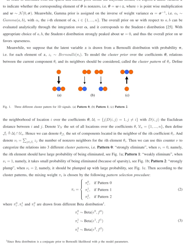
Meanwhile, we suppose that the latent variable z is drawn from a Bernoulli distribution with probability π, i.e. for each element of z, zi ∼ Bernoulli(πi). To model the cluster prior over the coefficients θ, relations
between the current componentθi and its neighbors should be considered, called the cluster pattern ofθi. Define
Fig. 1. Three different cluster pattern for 1D signals. (a) Pattern 0; (b) Pattern 1; (c) Pattern 2.
the neighborhood of location i over the coefficients θ,Ui ={j|D(i, j) = 1, j 6= i} with D(i, j) the Euclidean
distance between i andj. DenoteVN the set of all locations over the coefficientsθ,Vn ={1, ..., n}, then define
Ji,Ui∩Vn. Hence we can denoteθJi the set of components located in the neighbor of theith coefficientθi. And
denoteνi=Pj∈Jizj the number of nonzero neighbors for theith elementθi. Then we can use this counterν to
categorize the relations into 3 different cluster patterns, i.e. Pattern 0: “strongly eliminate”, whenνi= 0, namely,
theith element should have large probability of being eliminated, see Fig. 1a; Pattern 1: “weakly eliminate”, when
νi = 1, namely, it takes small probability of being eliminated (because of sparsity), see Fig. 1b; Pattern 2: “strongly
plump”, when νi= 2, namely, it should be plumped up with large probability, see Fig. 1c. Then according to the
cluster patterns, the mixing weightπi is chosen by the following pattern selection procedure:
πi= π0 i, if Pattern 0 π1 i, if Pattern 1 π2 i, if Pattern 2 (2) whereπ0 i, π 1 i andπ 2
i are drawn from different Beta distribution1.
π0 i ∼Beta(e 0 , f0 ) π1 i ∼Beta(e 1 , f1 ) π2 i ∼Beta(e 2 , f2 ) (3)
In order to clarify the dependance between the random variables, the distributions for π could be rewritten as follows: πi|e,f,zJ i ∼p(πi| e,f, zJi) (4) wheree,{e0 , e1 , e2 },f ,{f0 , f1 , f2 }.
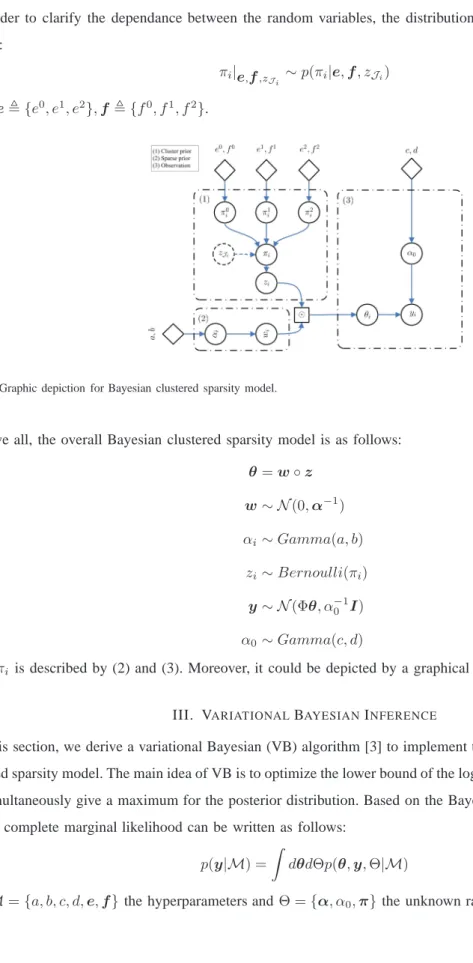
Fig. 2. Graphic depiction for Bayesian clustered sparsity model.
Above all, the overall Bayesian clustered sparsity model is as follows:
θ=w◦z w∼ N(0,α−1) αi∼Gamma(a, b) zi∼Bernoulli(πi) y∼ N(Φθ, α−1 0 I) α0∼Gamma(c, d) (5)
whereπi is described by (2) and (3). Moreover, it could be depicted by a graphical model in Fig. 2.
III. VARIATIONALBAYESIANINFERENCE
In this section, we derive a variational Bayesian (VB) algorithm [3] to implement the inference for the Bayesian clustered sparsity model. The main idea of VB is to optimize the lower bound of the log marginal likelihood function, and simultaneously give a maximum for the posterior distribution. Based on the Bayesian clustered sparsity model (5), the complete marginal likelihood can be written as follows:
p(y|M) = Z
dθdΘp(θ,y,Θ|M) (6)
In the following, we defineh·ix the expectation with respect to random variables2 x, x˜ the updated estimation
for random variablex, andy−k =y−
P
i6=kziwiφi the contribution of thek-th element of sparse signal on the
measurementy.
A. The VB-E Step 1) Update forw: q(w)∼ exp h n X i=1 lnp(wi|αi)iαi ! exp (hlnp(y|w,z, α0)iz,α0)
The posterior of w can be shown to be multivariate Gaussian distribution, with mean µ and variation Σ, i.e.,
˜
w∼ N(µ,Σ), with
Σ = ( ˜A+ ˜α0hZΦTΦZi)−1 µ= ˜α0Σ ˜ZΦTy
(7)
whereA=diag(α)andZ=diag(z). And given the updated valuez˜, we can derive
hZΦTΦZ
i= (ΦTΦ)
◦ ˜z˜zT +diag(˜z◦(1−z˜)
Consequently, we can derive the update forw as follows:
˜
w=µ (8)
2) Update forz: For each element ofz, the posterior could be given as
q(zi)∼exp(hlnp(zi|πi)iπi) exp(hlnp(y−i|zi, wi, α0)iwi,α0)
Thus the probability thatzi= 1 is proportional to
p(zi= 1) ∼exp (hlnπii) exp −α˜20(hw2 iiφ T iφi−2 ˜wiφTi y−i) (9) wherehw2 ii= ˜w 2
i+σii withσiithei-th element of diagonal entries ofΣ. The probability thatzi= 0is proportional
to
p(zi = 0)∼exp(hln(1−πi)i) (10)
where the update forπi could be referred in (17) in following subsections.
Thus, the update forz can be easily obtained
˜ zi=
p(zi= 1)
p(zi= 0) +p(zi = 1)
(11)
B. The VB-M Step
1) Update forα: For each element ofαi, the posterior could be given as
q(αi)∼p(αi|a, b) exp(hlnp(wi|αi)iwi) ∼Gamma(αi|a′, b′) (12) with a′=a+1 2, b′=b+hw 2 ii 2
where the conjugate property between Gamma prior and Gaussian distribution is used. Thus, the update forαi is
obtained: ˜ αi=a′/b′ (13) 2) Update forα0: q(α0)∼p(α0|c, d) exp (hlnp(y|w,z, α0)iw,z) ∼Gamma(α0|c′, d′) (14) with c′ =c+m 2, d′ =d+hky−Φ(w◦z)k 2 iw,z 2
where the conjugate property between Gamma prior and Gaussian distribution is used. And given the updated value ofw,z, the expectation could be derived:
hky−Φ(w◦z)k2 iw,z =yTy−2( ˜w◦z˜)TΦT y+IT[hzzTi ◦ hwwTi ◦(ΦTΦ)] I (15) wherehzzT i= ˜zz˜T +diag(˜z◦(1−z˜))andhwwT i= ˜ww˜T + Σ. Thus the update forα0 could be obtained:
˜
α0=c′/d′ (16)
3) Update for π: For each of the πi, given the updated value for z, then we can easily calculate portion of
sparsity pattern effecting on πi:
p(Pattern 0) = (1−z˜i−1)(1−z˜i+1) p(Pattern 1) = ˜zi−1(1−z˜i+1) + (1−z˜i−1)˜zi+1 p(Pattern 2) = ˜zi−1˜zi+1
Thus the posterior ofπij, withj denoting the sparsity pattern, could be written as:
q(πji)∼p(π j i|e j , fj) exp(hlnp(zi|π j i)izi) ∼Beta(πij|e ′j i , f ′j i )
where e′ij=e j+p(Patternj)˜z i fi′j=fj+p(Patternj)(1 −z˜i) thus hlnπjii=ψ(e ′j i )−ψ(e ′j i +f ′j i ) hln(1−πji)i=ψ(f ′j i )−ψ(e ′j i +f ′j i ) whereψ(x) = d
dxln Γ(x)is a digamma function, and then the update forπi could be obtained:
hlnπii= 2 X j=0 p(Patternj)hlnπiji hln(1−πi)i= 2 X j=0 p(Patternj)hln(1−πij)i (17)
C. Summary of the algorithm and acceleration
Given observationyand sensing matrixΦ, the algorithm could be summarized as Algorithm 1.
Algorithm 1 CS for Cluster Structured Sparse Signals via VB
Initialization The hyperparametersM={a, b, c, d,e,f}, the pre-estimatedw(0) = ΦTy,z(0) = w
maxw, a stop criterionC.
1: repeat
2: Update unknown parameters via equations (13), (16) and (17):
˜
Θ ={α,˜ α˜0,π˜}
3: Update latent parameters via equations (8) and (11):
˜
x={w˜,z˜}
4: untilC
At the iterationt, define the residual as
Res(t) =ky−Φ˜θ(t)k
thus
C,Res(t)6√mσ0 whereσ0 is the invariance of noise.
1) Comparison to BCS: In the framework of BCS, the inverse problem (reconstruction) is solved by a Sparse
Bayesian Learning (SBL) [24], which has been proven to be capable to find the unique sparse solution (Theorem 2 and 3 in [24]).
On the other hand, by setting z ≡ 1, the proposed model would degenerate into BCS model, i.e. without consideration on clusters. Roughly, BCS model could be considered as a special case of Bayesian clustered sparsity model, where the prior on clusters provides a guidance of how to assign the priority of choosing bases: “considering first your neighbors”. While, in BCS model, this priority does not exist. Consequently, the performance of the proposed algorithm is at least as good as that of BCS and the worst case is when all significant entries of sparse signal are distributed isolated.
2) Acceleration: In the current form, the algorithm requires an inverse problem to update the value ofΣ, which is ann×nmatrix, and thus requires anO(n3)operations. This can be problematic since in cases of large length of signals,nmight be quit large. To alleviate this problem, we compute theΣas follows:
Σ = ( ˜A+ ˜α0hZΦTΦZi)−1
= ( ˜A+ ˜α0Z˜ΦTΦ ˜Z+diag(˜z◦(1−˜z))◦(ΦTΦ))−1
= (B+ ˜α0Φ˜TΦ)˜ −1
(18)
where Φ = Φ ˜˜ Z and B = ˜A+diag(˜z◦(1−˜z))◦(ΦTΦ) which is a diagonal matrix, thus its inverse can be
easily computed by directly inverse the elements located at the diagonal,D=B−1. Then using the inverse identity property, it has Σ =D−DΦ˜T(α−1 0 I+ ˜ΦDΦ˜ T )−1˜ ΦD (19) where matrixα−01I+ ˜ΦDΦ˜ T is with dimension of m
×m, which reduces the operations toO(m3), withm
≪n.
IV. EXPERIMENTS
To distinguish the algorithm proposed in this paper from the former CluSS algorithm in [27], for simplicity, we denote the proposed algorithm as CluSS-VB. All the hyperparameters are fixed for every experiments as follows:
a=b=c=d= 1e−6,(e0, f0) = (1/3,2/3),(e1, f1) = (1/3,1/3) and(e2, f2) = (2/3,1/3). The following experiments are organized as follows. A first glance on the performance of CluSS-VB on synthetic cluster structured sparse signals is given. Afterwards, with respect to the oversampling rate, defined asm/s, we compare the recovery accuracy between CluSS-VB and other state-of-the-art CS algorithms, respectively, BP [14], CoSaMP [23], and Baysian Compressive Sensing (BCS) [22]. Then in order to verify the performance for mismatched models, we compare the reconstructions by each of the algorithms with augmenting number of clusters. Meanwhile, the robust to measurement noises is considered and an application on real musical signal is given.
In the following experiments, all sensing matrix are constructed through Gaussian ensemble with normalized row vectors. Moreover, if without clarifying, the measurements are corrupted by a white noise with variance
its reconstructionθˆ:
SNR= 20 log10 k θk
kθ−ˆθk (20)
A. General view
First, we shall give a glance on the performance of the proposed algorithm and show the basis selection procedure during iterations. The original sparse signal is generated with lengthn= 256, sparsity s= 30and clustersk= 2, where cluster information on sizes, locations and numbers is chosen totally randomly and thus is unknown3. Moreover, the spikes are randomly generated by Gaussian distribution which coincides with the sparsity model and onlym= 2s= 60measurements are obtained by random projections.
In Fig. 3, the inference ofz andw are shown along with the iterations. Apparently, the result shows that basis choosing priority is considering the neighbors first. The final result is shown in Fig. 4, where the convergence evolution for Res(t)is also shown. Moreover, the inference for measurement noise invarianceσˆ0= 0.0077, which coincides with the original setσ0= 0.01.
Meanwhile, we also exploit the other state-of-the-art algorithms (BP, CoSaMP, BCS) respectively to reconstruct the same sparse signal, shown in Fig. 5. From the comparison, except for CluSS-VB, all other algorithms cannot be able to reconstruct this sparse signal with onlym= 60measurements. On the other hand, like BCS, CluSS-VB can also provide “error bars” for the final reconstruction, which can be used to evaluate the confidence for the estimation. 0 100 200 0 0.5 1 0 100 200 −2 0 2 0 100 200 0 0.5 1 0 100 200 −2 0 2 0 100 200 0 0.5 1 0 100 200 0 0.5 1 0 100 200 −2 0 2 0 100 200 0 0.5 1 0 100 200 −2 0 2 0 100 200 −2 0 2
Fig. 3. Inference ofz(left column) andw(right column) along with iterations: (from top to bottom) 5, 10, 20, 40, 60 iterations.
3For Block-CoSaMP proposed in [2], it is impossible to recover this kind of cluster structured signals successfully, and thus we did not make
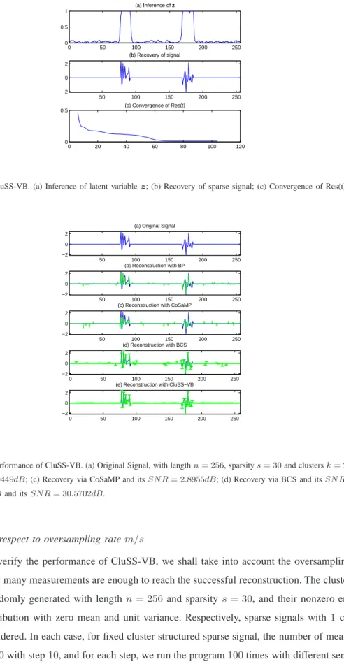
0 50 100 150 200 250 0 0.5 1 (a) Inference of z 50 100 150 200 250 −2 0 2 (b) Recovery of signal 0 20 40 60 80 100 120 0 0.5 (c) Convergence of Res(t)
Fig. 4. Performance of CluSS-VB. (a) Inference of latent variablez; (b) Recovery of sparse signal; (c) Convergence of Res(t).
50 100 150 200 250
−2 0 2
(a) Original Signal
0 50 100 150 200 250
−2 0 2
(e) Reconstruction with CluSS−VB
50 100 150 200 250 −2 0 2 (b) Reconstruction with BP 50 100 150 200 250 −2 0 2
(c) Reconstruction with CoSaMP
0 50 100 150 200 250
−2 0 2
(d) Reconstruction with BCS
Fig. 5. General view of performance of CluSS-VB. (a) Original Signal, with lengthn= 256, sparsitys= 30and clustersk= 2. (b) Recovery via BP and itsSN R= 7.0449dB; (c) Recovery via CoSaMP and itsSN R= 2.8955dB; (d) Recovery via BCS and itsSN R= 7.2022dB; (e) Recovery via CluSS-VB and itsSN R= 30.5702dB.
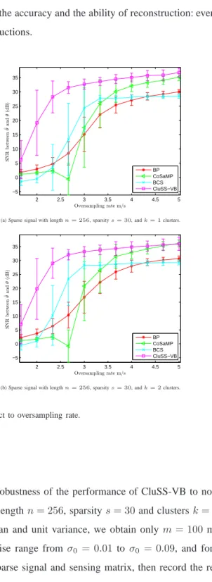
B. Performance with respect to oversampling ratem/s
In order to deeply verify the performance of CluSS-VB, we shall take into account the oversampling rate m/s, which determines how many measurements are enough to reach the successful reconstruction. The cluster structured sparse signals are randomly generated with length n= 256 and sparsitys= 30, and their nonzero entries drawn from a Gaussian distribution with zero mean and unit variance. Respectively, sparse signals with1 cluster and2
clusters are both considered. In each case, for fixed cluster structured sparse signal, the number of measurements is ranging from50to150with step10, and for each step, we run the program100times with different sensing matrix.
Fig. 6 shows the corresponding results, where (a) is for 1 cluster case and (b) is for 2 clusters case. The results show that CluSS-VB improves both the accuracy and the ability of reconstruction: even with very low oversampling rate, it can obtain desirable reconstructions.
2 2.5 3 3.5 4 4.5 5 −5 0 5 10 15 20 25 30 35 Oversampling rate m/s S NR b et w ee n ˆθa n d θ (d B ) BP CoSaMP BCS CluSS−VB
(a) Sparse signal with lengthn= 256, sparsitys= 30, andk= 1clusters.
2 2.5 3 3.5 4 4.5 5 −5 0 5 10 15 20 25 30 35 Oversampling rate m/s S NR b et w ee n ˆθa n d θ (d B ) BP CoSaMP BCS CluSS−VB
(b) Sparse signal with lengthn= 256, sparsitys= 30, andk= 2clusters.
Fig. 6. Performance comparison with respect to oversampling rate.
C. Robustness to noise
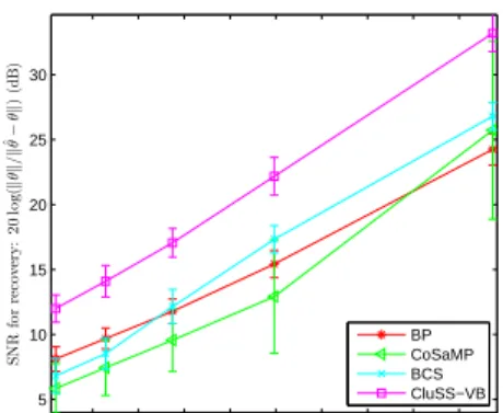
This experiment is to testify the robustness of the performance of CluSS-VB to noise (perturbations). Similarly, considering the sparse signals with lengthn= 256, sparsity s= 30and clustersk= 2and with nonzero elements drawn from Gaussian with zero mean and unit variance, we obtain only m= 100 measurements, corrupted by a white noise. Let the variance of noise range from σ0 = 0.01to σ0 = 0.09, and for each noise level, repeat the experiments100times with same sparse signal and sensing matrix, then record the recovery SNR. The results are shown in Fig. 7, and show that the SNR of CluSS-VB is proportional to the noise bound. Meanwhile, it is shown that with consideration of cluster structures, CluSS-VB exhaustively improves the recovery accuracy comparing to other algorithms.
14 16 18 20 22 24 26 28 30 5 10 15 20 25 30
SNR for observation: 20 log(kyk/kǫk) (dB)
S NR fo r re cov er y : 2 0 lo g( k θ k / k ˆθ− θ k ) (d B ) BP CoSaMP BCS CluSS−VB
Fig. 7. Robustness to different level of measurement noise.
D. Effects of clusters: mismatch models
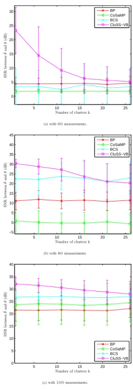
In this section, we will investigate the effects of clusters on the performance of CluSS-VB. Consider the sparse signals with length n = 256 and sparsity s = 30 and with nonzero elements drawn from Gaussian. Let the number of clusters k range from 1 to sparsity s, then for different oversampling rate, namely, measurements
m ∈ {60,80,100}, we repeat the experiments 100times for each number of clusters and each of oversampling rates. The results are shown in Fig. 8, where it shows that: with the number of clusters ascending, (1) the SNR of recovery by CluSS-VB is decreasing, (2) the variance of recovery by CluSS-VB is increasing, (3) while the SNR of recovery by other algorithms almost does not change. Even though the performance of CluSS-VB is decreasing, it still outperforms the other algorithms. This result also implies the robustness to mismatch models for CluSS-VB. And more interestingly, when the number of clusterskgoes to the sparsitys, the performance of CluSS-VB tends to converge to the performance of BCS, which coincides with the discussion in section III.
E. Experiments on real musical signals
In the last experiment, we apply the proposed algorithm on real musical signals, which have the property of cluster structured sparsity if considering signals in the frequency domain4, as shown in Fig. 9, where the significant spectrums are almost clustered together. We choose a clip of music of Mozart played by flute as the test example. The CS procedure is carried out piecewise with lengthn= 256for each of the pieces. Then varying the number of measurements obtained by random projections, fromm=⌊n/2⌋to⌊n/5⌋, corrupted by white noises with variance
σ0= 0.01, respectively, we use the different algorithms to recover the original musical signals piecewise from the compressed measurements and then concatenate the recovered pieces. As shown in Fig. 10, with onlym=⌊n/5⌋
measurements, the spectrograms of recovered signals are given for each algorithm. It is shown that CluSS-VB can desirably preserve the clusters of the original sparsity while suppress the isolated spikes, and hence can give better
5 10 15 20 25 0 5 10 15 20 25 30 Number of clusters k S NR b et w ee n ˆθa n d θ (d B ) BP CoSaMP BCS CluSS−VB
(a) with60measurements.
5 10 15 20 25 −5 0 5 10 15 20 25 30 35 40 45 Number of clusters k S NR b et w ee n ˆθa n d θ (d B ) BP CoSaMP BCS CluSS−VB (b) with80measurements. 5 10 15 20 25 0 5 10 15 20 25 30 35 40 Number of clusters k S NR b et w ee n ˆθa n d θ (d B ) BP CoSaMP BCS CluSS−VB (c) with100measurements.
Fig. 8. Effects of clusters on the performance.
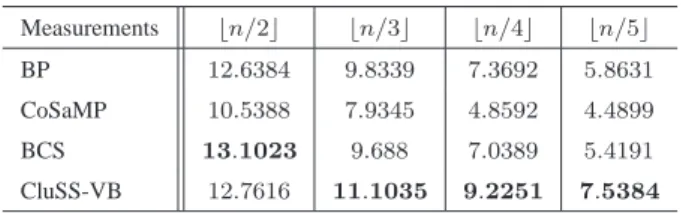
reconstructions with high recovery SNR. Meanwhile, we record the SNR for each of the algorithms with different level of oversampling rate, shown in Tab. II. The results show that CluSS-VB gives better reconstructions, especially with lower oversampling rate.
TABLE II
RECOVERYSNRFORDIFFERENTNUMBER OFMEASUREMENTS. (DB)
Measurements ⌊n/2⌋ ⌊n/3⌋ ⌊n/4⌋ ⌊n/5⌋ BP 12.6384 9.8339 7.3692 5.8631 CoSaMP 10.5388 7.9345 4.8592 4.4899 BCS 13.1023 9.688 7.0389 5.4191 CluSS-VB 12.7616 11.1035 9.2251 7.5384 0 1000 2000 3000 4000 5000 0.1 0.2 0.3 0.4 0.5 0.6 0.7 0.8 Frequency (Hz) Time
Fig. 9. Spectrogram of a musical signal.
Fig. 10. Spectrogram of reconstructions of musical signals via CluSS-VB (left-top), BCS top), BP (left-bottom) and CoSaMP (right-bottom).
V. CONCLUSION ANDPERSPECTIVES
In this paper, we proposed an algorithm, namely, CluSS-VB, to solve the cluster structured sparse signals from compressed measurements. Besides sparse prior, cluster prior on sparsity patterns are considered. Using a statistical
Bayesian graphical model, both priors are injected into a systematical Bayesian framework, where conjugate priors are exploited and results in an analytical solution from the variational Bayesian approach. Unlike the MCMC re-sampling inference, the global convergence (means always with energy descending for cost function) of CluSS-VB is guaranteed. Moreover, roughly, the cluster sparsity model could be considered as a generalization of BCS, and hence CluSS-VB will converge to BCS with mismatched models, i.e. spikes of sparse signals are randomly distributed (without cluster prior).
On the other hand, the theoretical guarantee for the sparse solution with CluSS-VB is not considered in this paper and thus still an open problem. Moreover, even though the algorithm is accelerated by reducing the dimension of the matrix involved into the inverse, an m×m inverse problem still needsO(m3)operations. Consequently, the acceleration of the algorithm needs to be considered in the future works.
REFERENCES
[1] S. D. Babacan, R. Molina, and A. K. Katsaggelos, “Bayesian compressive sensing using laplace priors,” IEEE Trans. Image Process., vol. 19, no. 1, pp. 53–63, 2010.
[2] R. G. Baraniuk, V. Cevher, M. F. Duarte, and C. Hegde, “Model-based compressive sensing,” IEEE Trans. Inf. Theory, vol. 56, no. 4, pp. 1982–2001, 2010.
[3] M. Beal, “Variational algorithms for approximate bayesian inference,” Ph.D. dissertation, Gatsby Computational Neuroscience Unit, University College London, 2003.
[4] C. M. Bishop, Pattern Recognition and Machine Learning (Information Science and Statistics). Secaucus, NJ, USA: Springer-Verlag New York, Inc., 2006.
[5] D. M. Blei, A. Y. Ng, and M. I. Jordan, “Latent dirichlet allocation,” J. Mach. Learn. Res., vol. 3, pp. 993–1022, March 2003. [Online]. Available: http://dx.doi.org/10.1162/jmlr.2003.3.4-5.993
[6] T. Blumensath and M. E. Davies, “Sampling theorems for signals from the union of finite-dimensional linear subspaces,” IEEE Trans. Inf.
Theory, vol. 55, no. 4, pp. 1872–1882, 2009.
[7] T. Blumensath, M. Yaghoobi, and M. E. Davies, “Iterative hard thresholding and l0 regularisation,” in Proc. IEEE International Conference
on Acoustics, Speech and Signal Processing ICASSP 2007, vol. 3, 15–20 April 2007, pp. III–877–III–880.
[8] E. J. Cand`es and T. Tao, “Decoding by linear programming,” IEEE Trans. Inform. Theory, vol. 51, no. 12, pp. 4203–4215, Dec. 2005. [9] ——, “Near-optimal signal recovery from random projections: Universal encoding strategies?” IEEE Trans. Inf. Theory, vol. 52, no. 12,
pp. 5406–5425, Dec. 2006.
[10] E. J. Cand`es and M. B. Wakin, “An introduction to compressive sampling,” IEEE Signal Process. Mag., vol. 25, no. 2, pp. 21–30, March 2008.
[11] V. Cevher, P. Indyk, L. Carin, and R. G. Baraniuk, “Sparse signal recovery and acquisition with graphical models,” IEEE Signal Proc
Mag, vol. 27, no. 6, pp. 92–103, 2010.
[12] V. Cevher, C. Hegde, M. F. Duarte, and R. G. Baraniuk, “Sparse signal recovery using markov random fields,” in Proc. Workshop on
Neural Info. Proc. Sys. (NIPS), 2008.
[13] V. Cevher, P. Indyk, C. Hegde, and R. G. Baraniuk, “Recovery of clustered sparse signals from compressive measurements,” in Int. Conf.
on Sampling Theory and Applications (SAMPTA), 2009.
[14] S. S. Chen, D. L. Donoho, and M. A. Saunders, “Atomic decomposition by basis pursuit,” SIAM Rev., vol. 43, no. 1, pp. 129–159, 2001. [15] D. L. Donoho, “Compressed sensing,” IEEE Trans. Inf. Theory, vol. 52, no. 4, pp. 1289–1306, Apr. 2006.
[16] Y. C. Eldar, P. Kuppinger, and H. Bolcskei, “Block-sparse signals: Uncertainty relations and efficient recovery,” IEEE Trans. Signal Process., vol. 58, no. 6, pp. 3042–3054, 2010.
[17] Y. C. Eldar and M. Mishali, “Robust recovery of signals from a structured union of subspaces,” IEEE Trans. Inf. Theory, vol. 55, no. 11, pp. 5302–5316, 2009.
[18] L. He and L. Carin, “Exploiting structure in wavelet-based bayesian compressive sensing,” IEEE Trans. Signal Process., vol. 57, no. 9, pp. 3488–3497, 2009.
[19] L. He, H. Chen, and L. Carin, “Tree-structured compressive sensing with variational bayesian analysis,” IEEE Signal Process. Lett., vol. 17, no. 3, pp. 233–236, 2010.
[20] J. Huang, T. Zhang, and D. Metaxas, “Learning with structured sparsity,” in The 26th International Conference on Machine Learning,
ICML09, Montreal, Quebec, Canada, June 2009.
[21] S. Ji, D. Dunson, and L. Carin, “Multitask compressive sensing,” IEEE Trans. Signal Process., vol. 57, no. 1, pp. 92–106, 2009. [22] S. Ji, Y. Xue, and L. Carin, “Bayesian compressive sensing,” IEEE Trans. Signal Process., vol. 56, no. 6, pp. 2346–2356, June 2008. [23] D. Needell and J. Tropp, “Cosamp: Iterative signal recovery from incomplete and inaccurate samples,” Applied and Computational
Harmonic Analysis, vol. 26, no. 3, pp. 301 – 321, 2009. [Online]. Available:
http://www.sciencedirect.com/science/article/B6WB3-4T1Y404-1/2/a3a764ae1efc1bd0569dcde301f0c6f1
[24] D. P. Wipf and D. D. Rao, “Sparse bayesian learning for basis selection,” IEEE Trans. Signal Process., vol. 52, no. 8, pp. 2153–2164, August 2004.
[25] M. E. Tipping, “Sparse bayesian learning and the relevance vector machine,” J. Mach. Learn. Res., vol. 1, pp. 211–244, 2001.
[26] J. A. Tropp and A. C. Gilbert, “Signal recovery from random measurements via orthogonal matching pursuit,” IEEE Trans. Inf. Theory, vol. 53, no. 12, pp. 4655–4666, Dec. 2007.
[27] L. Yu, H. Sun, J. P. Barbot, and G. Zheng, “Bayesian compressive sensing for cluster structured sparse signals,” Signal Processing