(IJSBAR)
ISSN 2307-4531
(Print & Online)
http://gssrr.org/index.php?journal=JournalOfBasicAndApplied
---
1
Statistical Downscaling Using Kernel Quantile Regression
to Predict Extreme Rainfall
Annisa Eki Mulyati
a*, Aji Hamim Wigena
b, Anik Djuraidah
cDepartment of Statistics, Faculty of Mathematics and Natural Science, Bogor Agriculture University, Bogor, West Java, Indonesia
aEmail: [email protected] bEmail: [email protected] cEmail: [email protected]
Abstract
Rainfall is one of climate elements with diverse intensity. In extreme circumtances it is necessary to study extreme rainfall to minimize impacts that may occur. Statistical downscaling is a method that can be used to predict rainfall, which is utilizing Global Circurlation Model (GCM) output data. The characteristics of GCM output data is curse of dimensionality which causes multicollinearity. Kernel trick is one method that can be used to overcome this problem by transforming GCM output data into a high-dimensional feature space. The transformation results are modeled with kernel quantile regression. This paper presents the use of kernel quantile regression to predict extreme rainfall, compared to kernel quantile regression with principal components. The result showed that based on the RMSEP values and the correlations, both models gave relatively similiar prediction.
Keywords: curse of dimensionality; kernel trick; quantile regression; rainfall; statistical downscaling.
1.Introduction
Predicting rainfall in certain area can use Statistical Downscaling (SD) which utilizes output data from the General Circulation Model (GCM).
--- * Corresponding author.
2
SD modeled the functional relationship between global scale GCM output data as predictors with local scale rainfall data as the response. GCM output data is curse of dimensionality which causes multicollinearity. The suitable model in SD leads to the use of data driven models as well as nonparametric models which do not require strict assumptions [1].Various SD models were developed for estimating rainfall including extreme rainfall such as using quantile regression models. This models can detect extreme conditions, both extreme dry at Q(0.5), and extreme wet at Q(0.75), Q(0.90) and Q(0.95) [2]. The curse of dimensionality can be overcome by reducing dimension using principal component analysis (PCA) [3], by using regularization such as elastic-net [4] and lasso [5]. Spline quantile regression with PCA can also detect extreme rainfall [6]. Besides these methods, the kernel SVM using PCA and Radial Basis Function (RBF) can predict the monthly rainfall in the dry season at Q(0.03), Q(0.18), Q(0.28), and Q(0.45) [7]. In this research, the monthly rainfall is predicted using quantile regression. Curse of dimensionality in GCM output data is solved by kernel trick.GCM output data is transformed into features high dimensional spaces with the Gaussian RBF kernel function. The implementation of kernel function with regularization in the features space is carried out to regulate the error components and regularization components to obtain the optimal lambda. The optimal lambda in kernel quantile regression is used to predict extreme rainfall. The kernel trick method with PCA is compared to the kernel trick without PCA.
2.Materials and Methods
2.1. Kernel Methods
Kernel method maps the data from an input space to high-dimensional feature space [8]. The application of high-dimensional data is difficult to understand in computation, so mapping is carried out implicitly. Implicit mapping 𝜙𝜙 means that it is only needed to know the kernel function used, without knowing the nonlinear mapping function. The algorithm which works in kernel is known as kernel trick, expressed in the form of multiplication of two vectors product dot products in the feature space, which is denoted as 〈∙,∙〉ℋ.
𝑘𝑘�𝐱𝐱𝑖𝑖,𝐱𝐱𝑗𝑗� = 〈𝜙𝜙(𝐱𝐱𝐢𝐢), 𝜙𝜙�𝐱𝐱𝐣𝐣�〉ℋ
= 𝜙𝜙(𝐱𝐱𝐢𝐢)𝑇𝑇𝜙𝜙�𝐱𝐱𝐣𝐣� (1)
where 𝐱𝐱𝑖𝑖 and 𝐱𝐱𝑗𝑗 are the data in the input space and 𝜙𝜙 is nonlinear mapping from the input space to the feature space shown in Figure 1.
(a) Input Space (b) Feature Space
3
The Kernel function has several types, such as Kernel Gaussian RBF [9]
𝑘𝑘(𝑥𝑥,𝑥𝑥′) = exp�−2𝜎𝜎12‖𝐱𝐱 − 𝐱𝐱′‖2� (2)
The advantage of using kernel tricks is to transform high-dimensional data so that it can solve various model problems. One of the problems is caused by curse of dimensionality which makes the parameter estimation process difficult [10].
Some disadvantages of using kernel tricks are (1) Mapping (𝜙𝜙) is carried out implicitly so that it loses the nature of its features, such as transformation and dimension. (2) Determining the suitable kernel type and kernel parameters in data does not have standard provisions, so it needs to be tested several times. (3) The greater the dimension to the feature space will increase the computation and storage costs.
2.2. Kernel Quantile Regression
Quantil regression is a statistical technique to model the quantile of conditional distribution in the response variable with explanatory variables [11]. The quantile regression (τ) uses the loss function as a solution of minimization
𝑙𝑙𝜏𝜏(𝜉𝜉) =�𝜏𝜏𝜉𝜉(𝜏𝜏 − jika 1)𝜉𝜉 jika 𝜉𝜉 ≥𝜉𝜉< 00 (3)
where 𝑙𝑙𝜏𝜏is a loss function in the quantile of 𝜏𝜏 ∈(0,1). Based on 𝑙𝑙𝜏𝜏 quantile regression is defined with optimization, it is
min𝑓𝑓∈ℋ1𝑛𝑛∑𝑛𝑛𝑖𝑖=1𝑙𝑙𝜏𝜏�𝑦𝑦𝑖𝑖− 𝑓𝑓0(𝑥𝑥𝑖𝑖)� (4)
to minimize the risk in equation (4) can be added with regularization
min𝑓𝑓∈ℋ𝑛𝑛1∑𝑛𝑛𝑖𝑖=1ρ𝜏𝜏�𝑦𝑦𝑖𝑖− 𝑓𝑓0(𝑥𝑥𝑖𝑖)�+𝜆𝜆𝜆𝜆(𝑓𝑓𝑘𝑘) (5)
where 𝜆𝜆(∙) penalty of the regression function to prevent overfitting, and 𝜆𝜆 is the parameter which controls 𝜆𝜆(∙). The parameter regularization of 𝜆𝜆 controls between the regularization components and error components.
The dual optimization problem in equation (5) can be solved by connecting it to the feature space written in the form of :
𝑓𝑓𝑘𝑘(𝑥𝑥) =〈ϕ(𝑥𝑥),𝑤𝑤〉 (6) Based on equation (6), the equation (5) will be the following form
minimize min𝑤𝑤,𝑏𝑏,𝜉𝜉(∗)𝐶𝐶 ∑𝑚𝑚𝑖𝑖=1𝜏𝜏𝜉𝜉𝑖𝑖−(1− 𝜏𝜏)𝜉𝜉𝑖𝑖∗+1
4
subject to �
𝑦𝑦𝑖𝑖− 〈𝜙𝜙(𝑥𝑥𝑖𝑖),𝑤𝑤〉 ≤ 𝜉𝜉𝑖𝑖
〈𝜙𝜙(𝑥𝑥𝑖𝑖),𝑤𝑤〉 − 𝑦𝑦𝑖𝑖≤ 𝜉𝜉𝑖𝑖∗
𝜉𝜉𝑖𝑖,𝜉𝜉𝑖𝑖∗≥0
where 𝜉𝜉𝑖𝑖is the upper limit of error and 𝜉𝜉𝑖𝑖∗is the lower limit of error from training data.Then, this dual problem is calculated by using Lagrange Multipliers, so that the solution is obtained as follows:
𝑤𝑤= ∑ 𝛼𝛼𝑛𝑛i=1 𝑖𝑖ϕ(𝑥𝑥𝑖𝑖) or 𝑓𝑓(𝑥𝑥) =∑𝑛𝑛𝑖𝑖=1𝛼𝛼𝑖𝑖𝐾𝐾(𝑥𝑥𝑖𝑖,𝑥𝑥)
where 𝐾𝐾(𝑥𝑥𝑖𝑖,∙) is kernel function of 𝑖𝑖𝑡𝑡ℎ from the training data, and 𝛼𝛼= (𝛼𝛼1, … ,𝛼𝛼𝑛𝑛)𝑇𝑇 with the assumption of kernel function coefficient vector.
3.Research Methods
3.1. Data
Response data in this research is monthly rainfall data from years 1981 to 2013 in Indramayu District. These data are in ZOM 79 including Krangkeng, Sukadana, Karangkendal, and Gegesik stations. GCM output data are from CMIP5 (multi-model ensemble Phase 5 Couple Model Intercomparisson Project) in the website http://pcmdi-cmip.llnl.gov/cmip5. Data are located at 1.25° LS - 18.75° LS and 101.25° BT - 118.75° BT, consisting of 8×8 grid [1]. The GCM data is used as explanatory variables, so there are 64 explanatory variables.
3.2. Methods
The methods in this reseacrh consist of the following steps :
1. Rainfall data exploration as preliminary information to observe the diversity of observational data. 2. Determining the time-lag of GCM data based on rainfall data using Cross Correlation Function (CCF)
[12].
3. Reducing dimension of GCM-lag data using PCA. The number of principal components based on the 95% cumulative proportion and the eigen values are greater than 1.
4. Dividing the data into training data and testing data. Based on training data four models are then developed to predict one year rainfall. The models are as follows :
a. Model 1 (M1) uses training data from 1981-2009 and testing data in 2010 b. Model 2 (M2) uses training data from 1981-2010 and testing data in 2011 c. Model 3 (M3) uses training data from 1981-2011 and testing data in 2012 d. Model 4 (M4) uses training data from 1981-2012 and testing data in 2013
5. Developing models uses R programs in the package “kernlab”. The steps are as the following:
a. Computation Kernel Gaussian RBF using function kernel “rbfdot” [13]. The value of𝜎𝜎 is estimed based on 10-fold cross validation in the training data.
5
b. Applying the regularization to obtain the optimal value of λ with try-and-error method as many as 40 experiments. It is started from 𝜆𝜆 =0.1 to𝜆𝜆=20 with increment of 0.5. The optimal 𝜆𝜆 is based on the minimum error value almost close to zero and not negative [14].
c. Developing kernel quantile regression based on the optimal λ for each Q(0.75), Q(0.90) and Q(0.95). The first model uses GCM-lag predictors without PCA and the second model uses GCM-lag predictors with PCA.
6. Measuring the model goodness of fit based on the correlation and Root Mean Square Error of Prediction (RMSEP) with the formula of �1
𝑛𝑛∑𝑛𝑛𝑖𝑖=1(𝑦𝑦𝑖𝑖− 𝑦𝑦�𝚤𝚤)2, where the value of 𝑛𝑛 is the number of
observations, 𝑦𝑦𝑖𝑖is the actual data and 𝑦𝑦�𝚤𝚤is the estimated value. 7. Testing the consistency of the four models (M1, M2, M3 and M4).
4.Results and Discussions
4.1. Data Exploration
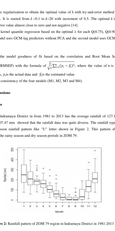
Monthly rainfall in Indramayu District in from 1981 to 2013 has the average rainfall of 127.19 mm and the standard deviation 107.47 mm showed that the rainfall data was quite diverse. The rainfall type in Indaramyu District is the Monsoon rainfall pattern like "U" letter shown in Figure 2. This pattern shows the clear differences between the rainy season and dry season periods in ZOM 79.
Figure 2: Rainfall pattern of ZOM 79 region in Indramayu District in 1981-2013
4.2. Kernel Quantile Regression
4.2.1. Kernel Quantile Regression using GCM-lag Predictors
The kernel quantile regression using GCM-lag predictors with regularization carried out by try-and-error method to determine the optimal lambda. The optimal lambda prevents overfitting, so that the model becomes
6
more accurate and more stable. The selected optimal lambda based on error changes close to zero and not negative. The lambda values of Q(0.75), Q(0.90) and Q(0.95) are different as presented in Table 1. This optimal lambdas are used to predict rainfall in 2013. The predicted rainfall are close to the actual rainfall shown in Figure 3.
Table 1: Optimal Lambda Values using GCM-lag Predictors
Quantile Lambda Error Error Change 0.75 10.0 0.103 0.00
0.90 3.0 0.075 0.00
0.95 2.0 0.058 0.00
Figure 3: Prediction of kernel quantile regression model without PCA for rainfall in 2013
4.2.2. Kernel Quantile Regression using PC predictors of GCM-lag
In previous studies, the quantile regression used PCA to solve curse of dimensionality in GCM data [3] and [6]. The number of principal components (PC) as predictors in the models are usually as many as four PCs of GCM-lag data. They are 1PC, 2PC, 3PC and 4PC. The selection of PCs are based on the total cumulative proportion of 95% and the feature eigen values are more than 1 shown in Table 2.
Table 2: Eigen value and Cumulative Proportion
PCs Eigen Values Diversity Proportion Cumulative Proportion 1PC 54.04 0.840 0.84 2PC 2.95 0.040 0.89 3PC 2.17 0.030 0.92 4PC 1.31 0.020 0.94 5PC 0.8 0.010 0.96 ⋮ ⋮ ⋮ ⋮ 64PC 0 0 1 0 200 400 600 1 2 3 4 5 6 7 8 9 10 11 12 Ra in fa ll ( m m ) Month Actual Q(0.75) Q(0.90)
7
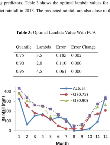
Kernel quantile regression is developed with four PCs as explanatory variables and rainfall as response variable. The process of optimal lambda determination in this model is the same as the process in kernel quantile regression using GCM-lag predictors. Table 3 shows the optimal lambda values for each quantil. This optimal lambdas are used to predict rainfall in 2013. The predicted rainfall are also close to the actual rainfall shown in Figure 4.
Table 3: Optimal Lambda Value With PCA
Quantile Lambda Error Error Change
0.75 3.5 0.185 0.002
0.90 2.0 0.110 0.000
0.95 4.5 0.061 0.000
Figure 4: Prediction of kernel quantile regression model withPCA for rainfall in 2013
4.2.3. Goodness of Fit Test
The goodness of fit of the two models are tested based on RMSEP and correlation between actual predicted rainfall (show in Table 4). Based on Table 4 both the model using GCM-lag predictors and the model using PC predictors of GCM-lag give relatively similar RMSEP and correlation value. The first model is better than second model because the first model does not need to dimension reduction, so the computation is simpler and faster.
Table 4: RMSEP and Correlation using GCM-lag and using PC of GCM-lag
Quantile GCM-lag PC of GCM-lag
RMSEP Correlation RMSEP Correlation
0.75 93.23 0.63 83.93 0.69 0.90 106.68 0.69 96.71 0.71 0.95 121.09 0.73 123.64 0.74 4.3. Consistency 0 100 200 300 400 1 2 3 4 5 6 7 8 9 10 11 12 Ra in fa ll ( m m ) Month Actual Q (0.75) Q (0.90)
8
The consistency of the model is necessary to know the prediction stability in different times [1]. Four rainfall models are validated based on the optimal lambda value by calculating RMSEP and the correlation in each quantile. Table 5 shows that the RMSEP of Q(0.75) on averages is lower than that of Q(0.90) and lower than that of Q(0.95). While, Table 6 shows that the average of correlation is about 0.7 and the standard deviation is about 0.13.
The rainfall predictions using both models are relative the same, so that both models are consistent in rainfall estimation.
Table 5: RMSEP of Kernel Quantile Regression using GCM-lag and using PC of GCM-lag
Model RMSEP GCM-lag PC of GCM-lag Q(0.75) Q(0.90) Q(0.95) Q(0.75) Q(0.90) Q(0.95) M1 (Year of 2010) 81.76 89.42 99.42 82.19 91.34 100.41 M2 (Year of 2011) 87.79 128.89 147.8 104.53 128.44 156.77 M3 (Year of 2012) 79.71 128.63 162.98 104.8 148.5 169.05 M4 (Year of 2013) 83.93 96.71 123.64 93.23 106.62 121.1 Average 83.3 110.91 133.46 96.18 118.72 136.83 Standard Deviation 3.46 20.82 27.88 10.78 25.02 31.67
Table 6: Correlation of Kernel Quantile Regression using GCM-lag and using PC of GCM-lag
Model Correlation GCM-lag PC of GCM-lag Q(0.75) Q(0.90) Q(0.95) Q(0.75) Q(0.90) Q(0.95) M1 (Year of 2010) 0.66 0.63 0.67 0.6 0.63 0.57 M2 (Year of 2011) 0.53 0.65 0.7 0.66 0.7 0.72 M3 (Year of 2012) 0.85 0.91 0.92 0.89 0.93 0.91 M4 (Year of 2013) 0.69 0.71 0.74 0.63 0.69 0.74 Average 0.68 0.72 0.76 0.7 0.74 0.73 Standard Deviation 0.13 0.13 0.11 0.13 0.13 0.14 5.Conclusions
Statistical Downscaling model using kernel quantile regression with GCM-lag predictors and the model with principal component predictors of GCM-lag predicted a relative similar extreme rainfall and consistent. The kernel quantile regression model using CGM-lag predictors was simpler and faster computation because the model did not need dimension reduction process.
References
9
peramalan curah hujan bulanan kasus curah hujan di Indramayu” [disertasi]. Bogor (ID): Institut Pertanian Bogor.
[2] Djuaridah A, Wigena AH. 2011. “Regresi Kuantil untuk Eksplorasi Pola Curah Hujan di Kabupaten Indramayu”. Jurnal Ilmu Dasar 12(1): 50-56
[3] Mondiana YQ. 2012. “Pemodelan statistical downscaling dengan regresi kuantil untuk pendugaan curah hujan ekstrim” [Tesis]. Bogor (ID): Institut Pertanian Bogor.
[4] Cahyani TBN, Wigena AH, Djuraidah A. 2016. “Quantile regression with elastic net in statistical downscaling to predict extreme rainfall”. Glob J Pure Appl Math. 12(4): 3517–3524.
[5] Zaikarina H, Djuraidah A, Wigena AH. 2016. “Lasso and ridge quantile regression using cross validation to estimate extreme rainfall”. Glob J Pure Appl Math. 12(3): 3305–3314.
[6] Goldameir NE, Djuraidah A, Wigena AH. 2015. “Quantile spline regression on statistical downscaling model to predict extreme rainfall in Indramayu”. Hikari J Appl Math Sci. 9(126):6263-6272.
[7] Khairunisa, Y. 2015. “Pemodelan Support Vector Machine Quantile Regression Untuk Prediksi Curah Hujan Bulanan Pada Musim Kemarau Studi Kasus Kabupaten Indramayu” [Thesis]. Bogor (ID): Institut Pertanian Bogor.
[8] Bousquet, Perez-Cruz. 2004. “Kernel Methods and Their Potential Use in Signal Processing”. IEEE Signal Processing Magazine. 21(3); 57-65
[9] Takeuchi I, Le QV, Sears T, Smola AJ. 2006. “Nonparametric Quantile Estimation”, Journal of Machine Learning Research 7: 1231-1264
[10] Bishop, C. M. 2006. “Pattern Recognition and Machine Learning”. New York: Springer
[11] Buhai S. 2005. “Quantile Regression Overview and Selected Application”. Ad Astra 4. Tersedia pada: www.ad-astra.ro/journal.
[12] Wigena AH, Djuraidah A, Sahriman S. 2015. “Statistical downscaling dengan pergeseran waktu berdasarkan korelasi silang”. JMG. 16(1):19-24.
[13] Karatzoglou A, Smola A, Hornik K, Zeileis A. 2004. “Kernlab-an S4 package for kernel methods in R. J Stat Softw”. 11(9): 1-20.
[14] Gagliardini P, Scaillet O. 2012. “Tikhonov regularization for nonparametric instrumental variable estimators”. J Econometics . 167(1): 61-75.