A toolbox for robust PID controller tuning using convex optimization

(1)

A toolbox for robust PID controller tuning

using convex optimization

Mehdi Sadeghpour, Vinicius de Oliveira and Alireza Karimi Laboratoire d’Automatique

Ecole Polytechnique F´ed´erale de Lausanne (EPFL) Lausanne, Switzerland

Abstract: A robust PID controller design toolbox for Matlab is presented in this paper. The design is based on linearizing or convexifying the conventional non-convex constraints on the classical robustness margins or H_∞ constraints. Then the existing optimization solvers can be used to compute the controller parameters. The software can be used in a wide range of controller design problems, including multi-model systems and gain-scheduled controllers. The models can be parametric or non-parametric while the software is compatible with the output data of the identiﬁcation toolbox of Matlab. Three illustrative examples exhibit convenience of working with the developed commands.

Keywords:Robust control, PID controller, convex optimization, toolbox 1. INTRODUCTION

PID controllers have become the most widely used type of controllers in practice. They are simple, effective con-trollers able to cover a large area of applications. Although the PID controller has only a three parameters to be tuned, it is surprisingly difficult to find the right tuning for them without systematic procedures and tools. To this end, a quite large variety of techniques and tools has been designed. Most of the techniques are useful in just special applications and cannot be considered a tool. The available tools, however, although having very good attributes, have at least one of these characteristics: 1) Using nonlinear and non-convex optimization problems in design, 2) not supporting multi-model systems, and 3) not considering

H∞ controllers for multi-model, either SISO or MIMO systems.

For instance in [Garpinger and Hagglund (2008)] a soft-ware tool for robust PID design is presented. But it uses a non-convex optimization method to design controllers and does not support multi-model cases. In [Oviedo et al. (2006)], a software package is proposed for tuning PID controllers based on constrained nonlinear optimization. The multi-model cases are not considered here either. Gonzalez-Martin et al. (2003) and Harmse et al. (2009) also provide useful PID tuning tools, however, multi-model systems is not supported and the methods are based on non-convex optimizations.

Few software tools have been presented so far that support multi-model cases. Most of them have not got the ﬁrst and/or third properties mentioned above. An example of these softwares is the one proposed by Bajcinca and Hulin (2004). This Matlab Toolbox designs PID or other three-term controllers based on the method of singular frequencies. But it cannot be used to design multivariable

H_∞ controllers. Another example is in Ge et al. (2002)

1 _{Corresponding author: Alireza Karimi}_{[email protected]}

where robust PID controllers are designed via Linear Matrix Inequalities (LMI) approach. This method does not support MIMO systems too.

According to what is said, there is not to the best of au-thors knowledge a PID controller design tool which designs robust controllers based on H_∞ or classical robustness margins for multi-model (SISO or MIMO) systems. In this paper, a quite comprehensive, yet simple and reliable robust PID controller toolbox for Matlab is presented. This toolbox designs robust controllers in terms ofH_∞ perfor-mance or classical robustness margins such as the gain and phase margin, for single/multi-model, either SISO or MIMO systems by solving linear or convex optimization problems. The software also supports the design of gain-scheduled PID controllers for LPV (Linear Parameter Varying) systems. The toolbox uses the YALMIP inter-face L¨ofberg (2004) for formulation of the optimization problems and the standard optimization solvers.

The paper is organized in ﬁve sections. In the next sec-tion, a concise theoretical basis for the commands of the software is presented. Section 3 is devoted to the expla-nation of the commands. In Section 4, three examples are provided, and Section 5 presents some conclusions.

2. THEORETICAL BASES

The underlying theories of the developed software are, in fact, the results of Karimi et al. (2007), Karimi and Galdos (2010), and Galdos et al. (2010). We shall briefly describe these results here in order to better understand the commands of the toolbox. Hence, first the class of con-trollers and models are presented and then different control performances that can be considered by the toolbox are given.

(2)

2.1 Class of models and controllers

The design method needs the frequency response of the plant model in a ﬁnite number of frequencies which can be obtained directly from data by spectral analysis or computed from a parametric model. Therefore, high order models with pure time delay and non minimum phase zeros can be considered with no approximation. We consider the set ofmmodels

M={Gi(jωk); i= 1, . . . , m, k= 1, . . . , N} (1)

where Gi(jωk) can be a scalar or a matrix representing

the frequency response of a SISO or MIMO model, respec-tively, at ω_k and N is large enough so that it will give a good approximation of the frequency response of the sys-tem. In the sequel a SISO model with a SISO controller is considered. Then, it will be shown how this method can be applied to compute multivariable decoupling controllers. The class of linearly parameterized controllers K=ρTφ, where ρ is the vector of controller parameters and φis a vector of basis functions is considered. A continuous-time PID controller belongs to this class with;

ρ= [kp ki kd]T , φ(s) = [1 1 s s 1 +τ s] T ₍₂₎

where k_p, k_i, and k_d are, respectively, the coeﬃcients of the proportional, integral, and derivative part of the PID controller and τ is the known time constant of the derivative part.

For a discrete-time PID controller, we have:

ρ= [k_p k_i k_d]T , φ(z) = [1 z

z−1

z ] T ₍₃₎

It is clear that higher order controllers can also be designed by the proposed approach with choosing for example a set of Laguerre basis functions for φ(see Karimi and Galdos (2010) for details).

The main interest of linearly parameterized controllers is that every point on the Nyquist diagram of the open loop transfer function is linear with respect to the controller parameters; i.e.,L(jωk) =ρTφ(jωk)G(jωk). This property

enables us to obtain linear or convex constraints for the optimization problems used in the controller design.

2.2 GPhC controller

Gain margin, phase margin and crossover frequency (GPhC) are typical performance specifications for PID controller design in industry. We use these specifications for SISO minimum-phase stable systems if the number of integrators in the open-loop transfer function is less than or equal to 2. Specifying the gain and phase margin defines a straight line in the Nyquist diagram (seed₁ in Fig. 1). Now, if the Nyquist curve of the open loop system lies in the right side ofd₁ the desired values for the gain margin

gm and phase margin ϕm will be assured. This can be

represented by a set of linear constraints thanks to the linear parameterization of the controller. Now, consider another straight line d2 which is tangent to the middle of the unit circle arc in the sector created by d₁ and the imaginary axis. If we call ωx the frequency at which the

Nyquist curve intersectsd₂, a crossover frequency greater than or equal toωxcan be achieved by a satisfying a set of

-1 Re Im β d₁ d2 ωx ω_c ϕm −1/gm

Fig. 1. GPhC speciﬁcations converted to linear constraints in Nyquist diagram

linear constraints. In fact, for frequencies greater thanωx

the Nyquist curve should lie belowd₁ and aboved₂ while for frequencies less thanωxit should lie belowd2. The control objective is to optimize the load disturbance rejection of the closed-loop. This is, in general, achieved by maximizing the controller gain at low frequencies. For continuous- and discrete-time PID controllers it corre-sponds to maximizingki[Karimi et al. (2007)].

Let us deﬁne the set of all points in the complex plane on the linedbyf(x+iy, d) = 0. Assume thatf(x+iy, d)<0 represents the half plane that excludes the critical point. Then, computing a controller that satisﬁes the desired performance can be carried out by the following linear optimization problem: maxki subject to: f(ρTφ(jωk)Gi(jωk), d1)<0 for ωk> ωx, f(ρTφ(jωk)Gi(jωk), d2)>0 for ωk> ωx, (4) f(ρTφ(jωk)Gi(jωk), d2)<0 for ωkωx, for i= 1, . . . , m

In many control problems a constraint on the controller gain at high frequencies can help reducing the large pick values of the control input. This can be achieved by a constraint on the magnitude of the controller gain at frequencies greater thanωh:

|ρTφ(jωk)|< Ku for ωk> ωh (5)

This constraint is convex but can be linearized by con-sidering a bound on the real and the imaginary part of

ρT_φ₍_jω

k) and including it into the above linear

program-ming optimization.

2.3 Loop shaping controller :

The performance speciﬁcation can be deﬁned by a desired open loop transfer function Ld(jω). A typical choice for

stable systems isLd(s) =ωc/s. If a desired reference model M is available,Ld can be computed asLd=M/(1−M).

Then, a PID controller can be designed by minimizing the following quadratic criterion:

(3)

-1

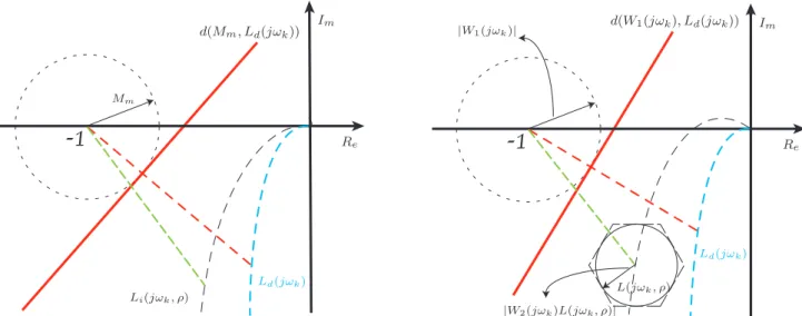
Mm Li(jωk, ρ) Ld(jωk) d(Mm, Ld(jωk)) Re Im

Fig. 2. Loop shaping in Nyquist diagram by quadratic programming J(ρ) = m i=1 N k=1 |Li(jωk, ρ)−Ld(jωk)|2 (6) whereL_i(jω_k, ρ) =ρT_φ₍_jω k)Gi(ωk).

The modulus margin, the shortest distance between the Nyquist curve and the critical point, is a better robustness indicator than the classical gain and phase margin [Landau et al. (2011)]. A modulus margin Mm of 0.5 is met if

the Nyquist curve does not intersect a circle of radius 0.5 centered at the critical point. This can be achieved if the Nyquist diagram is at the side ofd, a straight line tangent to the modulus margin circle, that excludes the critical point. This constraint is linear but conservative. The conservatism can be reduced if the slope of this line changes with the frequency. A good choice is a line

d(Mm, Ld(jωk)) orthogonal to the line that connects the

critical point and Ld(jωk) and tangent to the modulus

margin circle (see Fig 2). The controller can be designed solving the following quadratic optimization problem :

minJ(ρ)

f(ρTφ(jω_k)G_i(jω_k), d(M_m, L_d(jω_k)))<0 (7) for k= 1, . . . , N , for i= 1, . . . , m

This approach can be applied to unstable systems if Ld

contains the same number of unstable poles as well as the poles ofLi(s) on the imaginary axis (see Karimi and

Galdos (2010) for details).

2.4 H_∞ controller

Consider a SISO plant model with multiplicative unstruc-tured uncertainty: ˜G(jω) = G(jω)[1 +W₂(jω)∆] where

G(jω) is the plant nominal frequency function, W2(jω) is the uncertainty weighting frequency function, and ∆ is a stable transfer function with ∆_∞ < 1. In the Nyquist diagram the open loop frequency function will belong to a disk centered at L(jω, ρ) with a radius of

|W2(jω)L(jω, ρ)|. This disk can be approximated by a circumscribed polygon with p > 2 vertices: Li(jω, ρ) = K(jω, ρ)Gi(jω) fori= 1, . . . , p, where

-1

|W1(jωk)| |W2(jωk)L(jωk, ρ)| Ld(jωk) d(W1(jωk), Ld(jωk)) Re Im L(jωk, ρ)

Fig. 3. Expression of the robust performance condition as linear or convex constraints

G_i(jω) =G(jω) 1 +|W2(jω)| cos(π/p)e j2πi/p (8) Suppose that the nominal performance is deﬁned as

W1S∞ < 1, where S = (1 +KG)−1 is the sensitivity function andW₁is the performance weighting ﬁlter. This condition is satisﬁed if the Nyquist curve of the nominal model does not intersect the performance disk, a disk centered at the critical point with a radius of |W₁(jω)|. Therefore, the robust performance is achieved if there is no intersection between the uncertainty and performance disks [Doyle et al. (1992)]. This constraint can be linearized using a straight lined(W₁(jω), L_d(jω)) which is tangent to the performance disk and orthogonal to the line connecting the critical point andLd(jω) [Karimi and Galdos (2010)].

The robust performance is met ifLi(jω, ρ) is at the side of d(W₁(jω), Ld(jω)) that excludes the critical point for all ω. This can be represented by the following set of linear constraints:

f(ρTφ(jωk)Gi(jωk), d(W1(jωk), Ld(jωk)))<0 (9)

for k= 1, . . . , N , for i= 1, . . . , p

As a control objective the criterion in (6) can be mini-mized. An alternative is to deﬁne W₁S_∞ < γ as per-formance speciﬁcation and minimizingγ with a bisection algorithm.

In the same way, constraints on the weighted inﬁnity norm of other closed loop sensitivity functions can be included in the optimization problem (see more details in Karimi and Galdos (2010)):

W₃KS<1 , W₄GS<1 whereW₃ andW₄ are weighting ﬁlters.

2.5 MIMO controller

The performance speciﬁcations for SISO systems can also be used for designing MIMO controllers if the open loop system is decoupled. The main idea is to design a MIMO decoupling controller such that the open-loop transfer ma-trixL(jω) becomes diagonally dominant. For this reason a diagonal desired open loop transfer matrixL_dis consid-ered and the following quadratic criterion is minimized:

(4)

J(ρ) =

N

k=1

L(jω_k, ρ)−L_d(jω_k)_F (10) whereF stands for the Frobenius norm.

MIMO controllers presented by a matrix of transfer func-tions are considered, where each elementKijof the matrix

should be linearly parameterized, i.e., Kij =ρTijφij. The

controller parameters are obtained by minimizing J(ρ) under some constraints to meet the SISO speciﬁcations for each diagonal element.

In MIMO systems, besides the performance constraints, there are other constraints implying the stability of MIMO systems that should be considered. In fact, because the closed-loop system will not be completely diagonal, the stability of dominant loops will not guarantee the stability of the MIMO system. However, a stability condition can be obtained based on Gershgorin bands [Galdos et al. (2010)]:

r_q(ω_k, ρ)[1 +L_dq(jω_k)]−Re[1 +L_dq(−jω_k)] ×[1 +Lqq(jωk, ρ)] <0, for k= 1, . . . , N and q= 1, . . . , no (11) where r_q(ω, ρ) = no p=1,p=q |L_pq(jω, ρ)|,

n_o is the number of the outputs of the system andL_dq is theqth _{diagonal element of}_L

d.

2.6 Gain-scheduled controller

All presented robust controller design methods for systems with multimodel uncertainty can be extended to designing gain-scheduled controllers. Suppose that each model in (1) is associated to a value of a scheduling parameter vectorθ, which is measured in real time. The controller parameters can be polynomial functions ofθ and be computed by the optimization algorithm. For example, for a PID controller with a scalar scheduling parameter and the vector ρ a second order polynomial ofθwe have [Kunze et al. (2007)]:

ρ(θ) = kp2 kp1 kp0 ki2 ki1 ki0 kd2 kd1 kd0  θ 2 θ 1   3. TOOLBOX COMMANDS

There are three commands that constitute the software structure. The first command determines the controller structure. In the second command the control performance is defined, and finally the last command designs the con-troller with the predefined structure to meet the perfor-mance specifications. In the following comes a description of these three commands.

3.1 Controller structure

The controller structure is deﬁned by the vector of basis function φ. The command is of the form:

phi = conphi(ConType,ConPar,CorD,F)

ConType is a string specifying the type of the

con-troller and can take the following values: ‘PI’, ‘PD’,

‘PID’, ‘Laguerre’, ‘General’, where‘Laguerre’and

‘General’are used for higher order controller design using

Laguerre or generalized orthogonal basis functions and are not discussed in this paper.ConPardeﬁnes the parameters of the controller structure. For continuous-time PID and PD controllers, it is the time constant of the derivative ﬁlter, τ. It can be chosen such that −1/τ be a high frequency pole (the default value isτ = 1.2/ω_N).CorDis a string taking the values ‘s’ or ‘z’ showing that phi

must be a continuous or a discrete-time transfer function, respectively. Finally,‘F’is a transfer function that can be ﬁxed in the controller. For example, it can be the distur-bance model according to the internal model principle.

3.2 Control performance

The control performance is deﬁned by the following com-mand:

per = conper(PerType,par,Ld)

PerTypeis a string specifying the desired performance of

the system. It can be ‘GPhC’,‘LS’or ‘Hinf’, where LS stands for the loop shaping method.

The par for ’GPhC’ is a vector containing gain margin

gm, phase margin ϕm, crossover frequency ωc, maximum

of controller gainK_u and ω_h. No constraint for crossover frequency and maximum gain of controller is used if the last three values are missed. This type of performance can be used only for stable systems. If the desired Ld is speciﬁed, the criterion (6) will be minimized, else the low frequency gain of the controller will be maximized. Theparfor ‘LS’is a vector containingMm,Ku and ωh

and for ‘Hinf’ is a structure containing the weighting ﬁltersW₁,W₂,W₃ andW₄. These ﬁlters may be given as continuous- or discrete-time transfer functions or a vector of complex values in discrete frequencies. For ‘Hinf’,

par.gamma can be deﬁned as a vector containing γ_min,

γmax and . If this vector is speciﬁed the inﬁnity norm of the weighted sensitivity functions will be minimized by a bisection algorithm using the minimum and maximum value of γ with a tolerance of . If this vector is missed, the criterion (6) is minimized.

3.3 Controller design

The third and the last command is the main command in which an optimal controller of the speciﬁed structure in

phiwith the closed-loop desired performance characteris-tics of peris obtained. The general form of the command is as follows:

K=condes(G,phi,per,options)

whereKis the transfer function of the optimal controller.G

is the model of the system that can be atf,ss, or anfrd

object. In multi-model case, G must be deﬁned as a cell array,G{i}, which refers to the modelGi fori= 1, . . . , m.

options is a structure that deﬁnes diﬀerent options for

the controller optimization. For example, options.wis a vector of frequency points where frequency response of the system is known or is to be evaluated. If it is not speci-ﬁed by the user, a default grid for frequency is created. For gain-scheduled controller design options.gs=theta

(5)

should be assigned, wherethetais a vector (or matrix if we have more than one scheduling parameter) of the schedul-ing parameter values at which the constraints should be met and options.np=np is the order of the polynomial for the gain scheduled controller. The number of mod-els in G should be equal to the number of grid points

in theta. The optimization solver can be assigned by

options.solver=‘linprog’if linear programming solver

should be used.

In MIMO case, G is an no×ni matrix transfer function

where n_i is the number of inputs and n_o the number of outputs. The controller will be an ni ×no matrix

transfer function. If one wants to define different controller structure for different elements of matrix K, one should define phi as ann_o×n_i cell object. Then each element of phi can be created using the conphi command, for example in a loop. If phi is entered just as one vector, then it will be used for all elements of the controller matrix transfer functions. In the same way, per is defined for diagonal elements ofL=GK. Soper{i}{q}is a structure containing the desired performance characteristics of the

qth _{diagonal element of} _L

i = GiK if we have diﬀerent

performance speciﬁcation for each modelGi.

4. EXAMPLES

This section presents some examples of the use of the toolbox commands.

Example 1 Consider a system with three models in three diﬀerent operating points :

G₁(s) = 4e −3s 10s+ 1 ; G2(s) = e−5s s2+ 14s+ 7.5 G₃(s) = 2e −s 20s+ 1

Compute a PID controller for a gain margin of greater than 3 and a phase margin of at least 60◦ for all models. Specifying these margins, a controller with maximum performance in terms of load disturbance rejection is designed by entering the series of commands:

s=tf('s'); G{1}=exp(−3*s)*4/(10*s+1); G{2}=exp(−5*s)/(sˆ2+14*s+7.5); G{3}=exp(−s)*2/(20*s+1); phi=conphi('PID',0.05,'s'); per=conper('GPhC', [3,60]); K=condes(G,phi,per)

The PID controller is:

K(s) = 0.5326s

2_{+ 0}_.₅₂₁₄_s_{+ 0}_.₀₅₃₃₇

0.05s2+s (12)

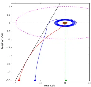
It should be noted that the gain and phase margin of the resulting open-loop system are greater or equal to the spec-iﬁed ones. The Nyquist curves of the three resulting open-loop transfer functions shown in Fig. 4 exhibit satisfaction of the constraints.

Example 2 Consider the system given in the previous example. The aim is to design a gain-scheduled PID controller with loop shaping method for this system.

−1 −0.5 0 0.5 −3.5 −3 −2.5 −2 −1.5 −1 −0.5 0 0.5 1 Real Axis Imaginary Axis

Fig. 4. The Nyquist diagrams of KG1 (blue line), KG2 (green line), and KG₃ (red line) in Example 1. The black line isd1.

Suppose that the three models corresponds to a normalized scheduling parameterθ∈ {−1,0,1}. We consider a desired open loop transfer function Ld(s) = ωc/s with ωc = 1

rad/s and a desired modulus margin ofM_m= 0.4. Assume that the gain-scheduled PID controller is described as follows: K(s) = [kp ki kd] [1 1 s s 1 +τ s] T wherek_p=k_p₁θ+k_p₀,k_i =k_i₁θ+k_i₀andk_d =k_d₁θ+k_d₀. Using the series of commands:

Ld=1/s;Mm=0.4;

phi=conphi('PID',0.05,'s'); per=conper('LS',Mm,Ld);

options.gs=[−1,0,1];options.np=1; K=condes(G,phi,per,options)

the coeﬃcients of the gain-scheduled PID controller are :

k_p= 1.4703θ+ 2.0138

ki= 0.1671θ+ 0.3249 (13) kd= 2.1845θ+ 3.1771

In Fig. 5 the Nyquist diagrams of the resulting open-loop transfer functions for three values of θ = −1,0,1 are shown. All three curves do not intersect the modulus margin circle and their distance toLd is minimized.

Example 3 In this example, a PID controller for the multi-model MIMO process proposed in Bao et al. (1999) is designed. In Bao et al. (1999) a multi-loop PID controller is designed for the processG1(s) with weighting functions

W₁(s) and W₂(s). Afterwards, the designed controller is examined on a slightly diﬀerent system (denoted by

G₂ here) to check its robustness. The related transfer functions are:

(6)

−1.5 −1 −0.5 0 0.5 −1 −0.8 −0.6 −0.4 −0.2 0 0.2 0.4 0.6 Real Axis Imaginary Axis

Fig. 5. The Nyquist curves ofK(jω, θ)G(jω, θ) forθ=−1 (blue line), θ = 0 (green line), and θ = 1 (red line). The modulus margin of 0.4 is shown with a black circle. G₁(s) =   −33.89 (98.02s+ 1)(0.42s+ 1) 32.63 (99.6s+ 1)(0.35s+ 1) −18.85 (75.43s+ 1)(0.30s+ 1) 34.84 (110.5s+ 1)(0.03s+ 1)   G₂(s) =    −33.89 e−0.1s (98.01s+ 1)(0.43s+ 1) 32.63 e−0.1s (98.5s+ 1)(0.33s+ 1) −18.85 e−0.1s (76.0s+ 1)(0.31s+ 1) 34.84 e−0.1s (109.5s+ 1)(0.025s+ 1)    W₁(s) = s+ 1000 1000s+ 1I W2(s) = 500s+ 1000 3s+ 5000 I

Here, the weighting functions W₁ andW₂ are applied to both systemsG₁andG₂where a simple desired open loop function L_d is chosen as shown by the commands below:

s=tf('s'); Ld=1/(10*s); par.W1=(s+1000)/(1000*s+1); par.W2=(500*s+1000)/(3*s+5000); G{1}=G1; G{2}=G2; phi=conphi('PID',0.05,'s'); per=conper('Hinf',par,Ld); K=condes(G,phi,per)

The result is the following controller:

K(s) =    −10.83s2−17.12s−0.103 0.05s2+s −1.301s2+ 12.31s+ 0.1239 0.05s2+s −2.332s2−10.54s−0.05149 0.05s2+s 1.132s2+ 17.15s+ 0.09748 0.05s2+s   

In Bao et al. (1999) the proposed multi-loop controller could not satisfy the nominal performance condition

W₁S_∞ < 1 while our controller satisﬁes the robust performance condition for both models.

5. CONCLUSIONS

A Matlab toolbox for designing robust PID controllers is presented. This toolbox designs robust PID controllers using linear programming and in some cases convex opti-mization. When designing controllers based on constraints on classical robustness margins orH_∞ performance, solv-ing linear or convex optimization problems would be a

great advantage yielding faster and reliable results. Deal-ing with multi-model, either SISO or MIMO systems is easy with the presented toolbox. Three main commands are developed for design as shown in examples. A GUI will also be designed for the software to become more convenient to use.

REFERENCES

Bajcinca, N. and Hulin, T. (2004). Robsin: A new tool for robust design of PID and three-term controllers based on singular frequencies. InProceedings of the IEEE In-ternational Conference on Control Applications, 1546– 1551. Taipei, Taiwan.

Bao, J., Forbes, J.F., and McLellan, P.J. (1999). Robust multiloop PID controller design: A successive semideﬁ-nite programming approach.Industrial and Engineering Chemistry Research, 38(9), 3407–3419.

Doyle, C.J., Francis, B.A., and Tannenbaum, A.R. (1992). Feedback Control Theory. Mc Millan, New York. Galdos, G., Karimi, A., and Longchamp, R. (2010). H_∞

controller design for spectral MIMO models by convex optimization. Journal of Process Control, 20(10), 1175 – 1182.

Garpinger, O. and Hagglund, T. (2008). A software tool for robust PID design. InProceedings of the 17th IFAC World Congress. Seoul, Korea.

Ge, M., Chiu, M.S., and Wang, Q.G. (2002). Robust PID controller design via LMI approach. Journal of Process Control, 12(1), 3 – 13.

Gonzalez-Martin, R., Lopez, I., Morilla, F., and Pastor, R. (2003). Sintolab: the REPSOL-YPF PID tuning tool. Control Engineering Practice, 11(12), 14691480. Harmse, M., Hughes, R., Dittmar, R., Singh, H., and

Gill, S. (2009). Robust optimization-based multi-loop PID controller tuning: A new tool and an industrial example. In 7th IFAC International Symposium on Advanced Control of Chemical Processes, ADCHEM’09, 548–553. Istanbul, Turkey.

Karimi, A. and Galdos, G. (2010). Fixed-order H_∞

controller design for nonparametric models by convex optimization. Automatica, 46(8), 1388–1394.

Karimi, A., Kunze, M., and Longchamp, R. (2007). Ro-bust controller design by linear programming with ap-plication to a double-axis positioning system. Control Engineering Practice, 15(2), 197–208.

Kunze, M., Karimi, A., and Longchamp, R. (2007). Gain-scheduled controller design by linear programming. In European Control Conference, 5432–5438.

Landau, I.D., Lozano, R., M’Saad, M., and Karimi, A. (2011). Adaptive Control: Algorithms, Analysis and Applications. Springer-Verlag, London.

L¨ofberg, J. (2004). YALMIP: A toolbox for modeling and optimization in MATLAB. InCACSD Conference. URL

http://control.ee.ethz.ch/ joloef/yalmip.php.

Oviedo, J.J.E., Boelen, T., and Overschee, P.V. (2006). Robust advanced PID control (RaPID): PID tuning based on engineering speciﬁcations. IEEE Control Sys-tems Magazine, 26(1), 15–19.