Tobias Gerstenberg
*, Matthew F. Peterson
Department of Brain and Cognitive Sciences, Massachusetts Institute of Technology
Noah D. Goodman
Departments of Psychology and Computer Science, Stanford University
David A. Lagnado
Experimental Psychology, University College London
Joshua B. Tenenbaum
Department of Brain and Cognitive Sciences, Massachusetts Institute of Technology
Abstract
How do people make causal judgments? What role, if any, does counterfac-tual simulation play? Counterfaccounterfac-tual theories of causal judgments predict that people compare what actually happened with what would have hap-pened if the candidate cause had been absent. Process theories predict that people focus only on what actually happened, to assess the mechanism linking candidate cause and outcome. We tracked participants’ eye move-ments while they judged whether one billiard ball caused another one to go through a gate or prevented it from going through. Both participants’ looking patterns and their judgments demonstrated that counterfactual sim-ulation played a critical role. Participants simulated where the target ball would have gone if the candidate cause had been removed from the scene. The more certain participants were that the outcome would have been dif-ferent, the stronger their causal judgments. These results provide the first direct evidence for spontaneous counterfactual simulation in an important domain of high-level cognition.
Keywords: causality; counterfactuals; mental simulation; intuitive physics; eye-tracking.
*
Corresponding author: Tobias Gerstenberg ([email protected]), MIT Building 46-4053, 77 Massachusetts Avenue, Cambridge, MA 02139.
Introduction
In soccer, scoring an own goal is probably the worst thing that can happen to a player. An own goal occurs when a defender tries to prevent the other team from scoring but instead deflects the ball into his or her own team’s goal, thereby scoring a point for the other team. Simply having touched the ball last, however, is not sufficient to be “awarded” an own goal. Only when the ball was not already on target does the play count as an own goal. This kind of counterfactual reasoning is pervasive in sports. To take another example, in American football, pass interference is called when a defender illegally interferes with a receiver and thereby prevents him or her from making an attempt at catching a pass. However, the pass-interference rule does not apply when a referee deems the pass uncatchable. The defender’s action must have made a difference to the outcome. Of course, counterfactuals arise not only in sports. We use them to make sense of history (Ferguson, 2000), to determine causation in the law (Hart and Honoré, 1985), and to understand our own and other people’s actions and emotions (Alicke et al., 2015; Kahneman and Miller, 1986; Roese, 1997). We ponder over near misses (Kahneman and Varey, 1990) and regret decisions that could have turned out better (Loomes and Sugden, 1982; Zeelenberg et al., 1998).
The relationship between counterfactuals and causation has been a topic of long-standing debate in philosophy (Beebee et al., 2009; Hiddleston, 2005; Paul and Hall, 2013), psychology (Lipe, 1991; Walsh and Sloman, 2011; Wolff, 2007), and the law (Hart and Hon-oré, 1985; Schaffer, 2010; Stapleton, 2008). In philosophy, there are two broad theoretical frameworks for thinking about causation: Process theories (e.g. Dowe, 2000) analyze cau-sation in terms of spatiotemporally continuous processes that link causes to their effects. For example, when asked whether one billiard ball (A) caused another ball (B) to move, a process theorist would seek to establish whether a physical quantity (such as momentum) was transferred from ball A to ball B. In contrast,counterfactual theoriescapture causation by establishing whether the candidate cause made a difference to the outcome. A counter-factual theorist would say that A caused B to move because B would not have moved if A had not been there (Lewis, 1973). Previous empirical work on how people make causal judgments has yielded mixed results. Sometimes, participants’ judgments are influenced by information about causal processes (Lombrozo, 2010; Walsh and Sloman, 2011; Wolff, 2007), whereas at other times, participants care mostly about what would have happened if the cause had been absent (Gerstenberg et al., 2012, 2014).
Past research has shown that counterfactual thoughts are triggered when experienced outcomes are negative, unexpected, or close to alternative outcomes (Roese, 1997). Re-searchers have employed different methods to study spontaneous counterfactual thinking, such as having participants list their thoughts (Sanna and Turley, 1996) or measuring the speed with which they respond to different counterfactual statements (Roese and Olson,
1997). However, counterfactual thinking has never been shown directly. In this article, we demonstrate how eye-tracking can be used to uncover evidence for a particular kind of counterfactual thinking, which we refer to as counterfactual simulation (Crespi et al., 2012; Johansson et al., 2006; Hegarty, 1992; Kahneman and Tversky, 1982). As a case study, we focus on how people make causal judgments about physical interactions. We show that people’s causal judgments mirror how own goals are decided in soccer: People compare what actually happened with what would have happened in the counterfactual situation in which the candidate cause was absent.
We first describe the experimental paradigm we used in our study and then discuss model predictions separately for each experimental condition. In the Results section, we report our analyses of participants’ judgments, their eye movements, and the relationship between their eye movements and judgments. We conclude by discussing the implications our findings have for theories of causal judgment specifically, and for causal cognition more generally.
Experimental Paradigm
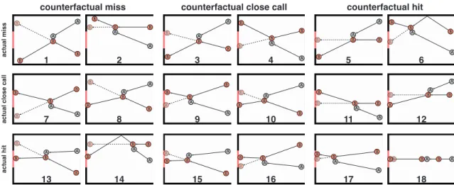
In our experiment, participants watched video clips in which two balls, A and B, collided with each other (see Fig. 1).1 The clips differed in whether ball B subsequently went through a gate (actual hit), barely went through the gate or missed the gate by a very small distance (actual close call), or missed the gate by a larger distance (actual miss). The clips also differed in what would have happened if ball A had not been present in the scene. Ball B would have clearly missed the gate (counterfactual miss), it would have just gone through or nearly gone through (counterfactual close call), or it would have clearly gone through the gate (counterfactual hit). For example, in Clip 3, ball B clearly missed the gate in the actual situation (actual miss) and would have just missed the gate in the counterfactual situation in which ball A was not present in the scene (counterfactual close call).
In a between-subjects design, we varied whether participants answered (a) a counter-factual question about what would have happened, (b) a causal question, or (c) a question about the actual outcome. Participants in the counterfactual condition rated the extent to which they agreed with the statement “ball B would have gone through the gate if ball A had not been present in the scene.” In thecausal condition, participants judged the extent to which they agreed with the statement “ball A caused ball B to go through the gate” (when ball B went through the gate) or the statement “ball A prevented ball B from going through the gate” (when ball B did not go through the gate). We made sure to avoid any
1All data and materials, including analyses, videos, and additional plots, have been made publicly
B B B B B B 1 7 13 2 8 14 B B B B B B 3 9 15 4 10 16 B B B B B B 5 11 17 6 12 18 actual hit
actual close call
actual miss
counterfactual miss counterfactual close call counterfactual hit
A B A B B B A A B B A B B B A A B A B B A B A B B A B B B A A B A B B A B B B A A B A B B A B A B B B A A B B A B B B A B A A B B A B A B B A B B B A A B B B A A B B B A A B A B B
Figure 1. Diagrams illustrating the 18 test clips shown to participants. Solid arrows indicate the motion paths of balls A and B prior to their collision and the path of B’s motion after the collision. Dashed arrows indicate where ball B would have gone if ball A had not been present in the scene. From top to bottom, the rows show situations in which B clearly missed the gate (actual miss), just missed the gate or only just went through (actual close call), and clearly went through the gate (actual hit). From left to right, the column pairs show situations in which B would have clearly missed the gate if ball A had not been present (counterfactual miss), would have just missed the gate or would have only just gone through (counterfactual close call), and would have clearly gone through the gate (counterfactual hit). Note that the font size of the balls’ labels has been increased here for readability.
reference to counterfactual language in this condition. In the outcome condition, partici-pants were asked to indicate their agreement with the sentence “ball B completely missed the gate” (when B did not go in) or the sentence “ball B went through the middle of the gate” (when B went in). Participants in all three conditions responded on a scale from 0 (not at all) to 100 (very much).
Theoretical Predictions
In previous work (Gerstenberg et al., 2012, 2014), we developed the counterfactual simulation model, which predicts causal judgments by simulating what would have happened if the cause had been absent and then comparing this counterfactual outcome with what actually happened. In the case of physical causation considered here, we assume that observers make use of their intuitive understanding of physics to simulate what would have happened in the relevant counterfactual situation. In this section, we discuss the model’s predictions in the counterfactual and causal conditions, both for behavioral judgments and for eye movements. We also discuss a model that we developed to make predictions about participants’ judgments in the outcome condition.
Counterfactual condition
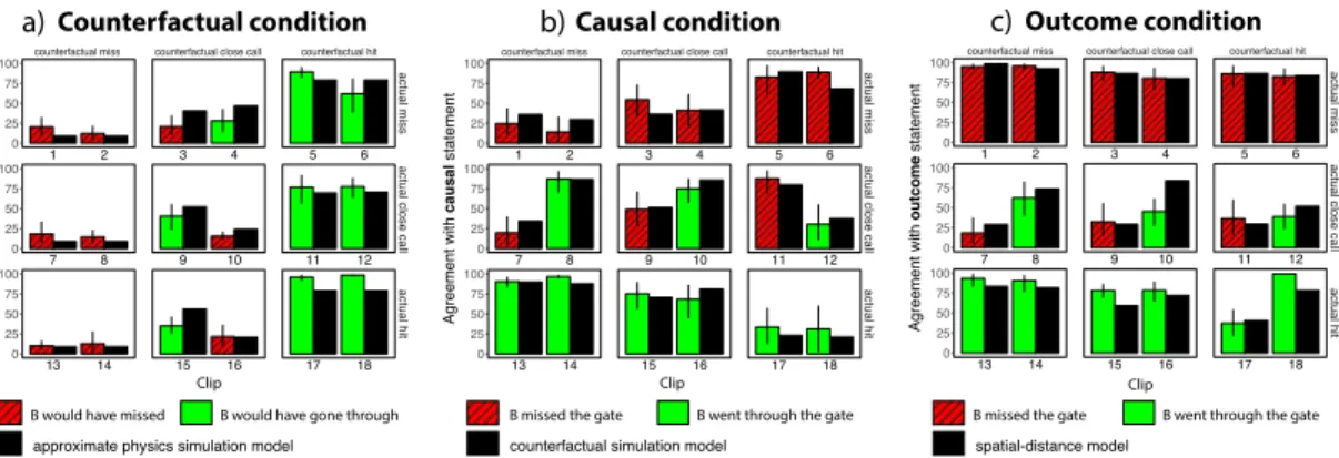
Our model assumes that participants make use of their intuitive understanding of physics to simulate what would have happened if ball A had not been present in the scene and also that this intuitive understanding takes the form of a “runnable mental model” (Craik, 1943) that can be implemented to a first approximation via the physics engine used to generate the stimulus clips (Gerstenberg et al., 2012, 2014; Gerstenberg and Tenenbaum, 2017; Goodman et al., 2015; Smith et al., 2013; Battaglia et al., 2013; Sanborn et al., 2013). Specifically, to capture participants’ uncertainty in whether ball B would have gone through the gate, the model generates noisy samples from the underlying physics engine that was used to generate the clips. In each sample, the model removes ball A from the scene, and introduces a small degree of Gaussian noise to ball B’s direction of motion at each time step in the physics simulation after the point at which the two balls would have collided. It is at this point in time that the counterfactual situation diverges from the actual situation that participants saw. For each sample, the model records whether ball B went through the gate, or missed it. We used the proportion of samples in which B went through the gate to predict participants’ counterfactual judgments. The black bars in Figure 2a show the predictions of this approximate physics simulation model predictions for the counterfactual condition. The model predicts that counterfactual judgments will be affected by how close the counterfactual outcome would have been (i.e., the columns in Fig. 1) but that how close the actual outcome was (i.e., the rows in Fig. 1) would make no difference.
Because participants were explicitly asked to judge whether ball B would have gone through the gate if ball A had not been present in the scene, we expected their eye move-ments to reveal attempts to extrapolate where ball B would have gone if ball A had not been present.
Causal condition
Given the results of our previous work (Gerstenberg et al., 2012, 2014), we expected a close correspondence between participants’ counterfactual and causal judgments. The black bars in Figure 2b show the predictions of the counterfactual simulation model of causal judgment. The model specifies the probability that a candidate cause C (ball A in our case) caused a particular outcome e (ball B going through the gate, or ball B missing the gate) as
P(C →e) =P(e0 6=e|S,remove(C)) (1) whereS represents the physical information about what actually happened, and e denotes the counterfactual outcome that would have happened if C had been removed from the scene. According to this model, participants’ agreement with the causal statement should
Causal condition b) 1 2 7 8 13 14 3 4 9 10 15 16 5 6 11 12 17 18 counterfactual miss counterfactual close call counterfactual hit
actual miss
actual close call
actual hit 0 25 50 75 100 0 25 50 75 100 0 25 50 75 100 Agreement with ca us al statement Clip 1 2 7 8 13 14 3 4 9 10 15 16 5 6 11 12 17 18 counterfactual miss counterfactual close call counterfactual hit
actual miss
actual close call
actual hit 0 25 50 75 100 0 25 50 75 100 0 25 50 75 100 Agreement with ou tc om e statement Outcome condition c) Clip B would have gone through
B would have missed
approximate physics simulation model
B went through the gate B missed the gate
counterfactual simulation model
B went through the gate B missed the gate
spatial-distance model a)Counterfactual condition Clip 1 2 7 8 13 14 3 4 9 10 15 16 5 6 11 12 17 18 counterfactual miss counterfactual close call counterfactual hit
actual miss
actual close call
actual hit 0 25 50 75 100 0 25 50 75 100 0 25 50 75 100 Agreement with co un te rfa ct ua l statement
Figure 2. Participant’s mean agreement judgments (0 = “not at all”, 100 = “very much”) and model predictions for each of the 18 video clips in the (a) counterfactual condition, (b) causal condition, and (c) outcome condition. In the counterfactual condition, participants were asked whether ball B would have gone through the gate if ball A had not been present; striped bars indicate situations in which ball B would have missed the gate, and solid bars indicate situations in which ball B would have gone through the gate. In the causal condition, participants were asked whether ball A prevented ball B from going through the gate when ball missed the gate (striped bars) or whether ball A caused ball B to go through the gate when ball B went through (solid bars). In the outcome condition, participants were asked whether ball B completely missed the gate when it did not go in (striped bars) or whether ball B went through the middle of the gate when ball B did go in (solid bars). Error bars indicate bootstrapped 95% confidence intervals.
increase the more certain they are that the outcome in the counterfactual situation (e0) would have been different from the actual outcome (e). In the analyses reported here, we used participants’ mean judgments in the counterfactual condition to determine the probability that the outcome would have been different for each clip, and then used these probabilities to predict participants’ mean judgments in the causal condition.2
For example, in Clip 1 (see Fig. 1), ball B missed the gate, and participants in the counterfactual condition believed that B would have missed the gate even if ball A had not
2
We would have also been able to use the predictions of the approximate physics simulation model, which captures participants’ counterfactual judgments, to get the counterfactual probabilities required by the counterfactual simulation model as detailed in Equation 1. However, because we asked participants in the counterfactual condition to judge whether they thought ball B would have gone through the gate if ball A had not been present in the scene, we instead directly mapped these ratings onto participants’ prevention judgments for the clips in which ball B missed the gate. The model predicts that prevention judgments should increase the more certain participants are that ball B would have gone through the gate. To predict participants’ causal judgments for situations in which ball B went through the gate, we subtracted participants’ counterfactual judgments in these situations from 100 (the maximum of the scale) to capture their belief that ball B would have missed the gate if ball A had not been present. Participants’ causal judgments when ball B went through the gate were predicted to increase the more certain they were that B would have missed the gate if ball A had not been present. More generally, whereas the approximate physics simulation model yields the probability of a particular counterfactual outcome, the counterfactual simulation model of causal judgment captures whether the counterfactual outcome would have been different from what actually happened.
been present in the scene (see Fig. 2a). Because the presence of ball A made no difference to whether ball B missed the gate, the model predicts that participants should indicate that ball A did not prevent ball B from going through (Fig. 2b). In Clip 5, ball B again did not go through the gate, but this time, participants were confident that it would have gone through if ball A had not been present. Thus, the model predicts that participants should indicate that ball A prevented ball B from going through the gate in this case. In Clip 9, ball B missed the gate, but participants in the counterfactual condition were less certain about what would have happened if ball A had not been present in the scene. Because it is unclear whether ball B would have gone through the gate if ball A had not been there (i.e., the counterfactual probability in Equation 1 is close to .5), the model predicts an intermediate rating.
The same relationship between participants’ confidence in ball A’s having made a difference to the outcome and their agreement ratings is also predicted for the situations in which ball B ended up going through the gate. The model predicts that agreement with the statement that ball A caused ball B to go through the gate should increase the more certain participants in the counterfactual condition were that ball B would have missed otherwise. In sum, we expected participants’ judgments in the causal condition to be influenced by the actual outcome (whether ball B went through or missed the gate) and by how clear it was what would have happened if ball A had been removed.
Given the hypothesized connection between causal judgments and counterfactual rea-soning, we predicted that participants in the causal condition would spontaneously engage in counterfactual simulation to gauge whether the outcome would have been different if the candidate cause had been removed from the scene. Thus, we expected to observe eye move-ments to where ball B would have gone if ball A had been absent, as in the counterfactual condition.
Outcome condition
To predict participants’ agreement judgments in the outcome condition, we developed a simplespatial-distance model that computes the euclidean distance between the center of the gate and the point at which ball B hit the wall or went through the gate. The model predicts that participants’ agreement ratings for situations in which ball B went through the gate should increase the closer ball B was to the center of the gate when it went through (see Fig. 2c). Agreement ratings for situations in which ball B missed the gate are predicted to increase the greater the distance was between the point at which ball B hit the wall and the center of the gate. The spatial-distance model predicts that participants’ judgments should be influenced only by the closeness of the actual outcome (i.e., the rows in Fig. 1) and not by the closeness of the counterfactual outcome (i.e., the columns in Fig. 1).
Judging how closely ball B was to the center of the gate when it went through or how far ball B was from the gate when it missed did not require simulating what would have happened if ball A had been absent. Thus, we predicted that participants in the outcome condition would be less likely to engage in counterfactual simulation than participants in the other two conditions. Accordingly, in the outcome condition, we expected to see fewer eye movements in the direction of where ball B would have gone if ball A had been absent. Method
Participants. Forty participants were recruited from the Massachusetts Institute of Technology’s participant pool and paid for their participation. We determined the target number of participants on the basis of our previous work (Gerstenberg et al., 2012), which established very strong behavioral effects in the counterfactual and causal conditions using the same materials employed in this study. A power analysis conducted with G*Power 3.1 (Faul et al., 2007) showed that fewer than 10 participants were required for .95 power to detect the weakest effect (f = 1.01) found in our previous work, given an level of .05. To have equal numbers of participants in the three conditions, we kept the 10 participants with the least amount of eye-tracking data loss (e.g., due to blinking, head movement, or looking away from the monitor) in each condition. The mean percentage of eye-tracking data loss after the removal of the additional participants was 9.39% (SD = 6.65) in the counterfactual condition, 7.31% (SD = 3.49) in the causal condition, and 8.27% (SD = 3.35) in the outcome condition. Thirty participants (mean age = 36 years, SD = 15.9; 9 female) were included in the analyses reported here.3
Design. Participants were randomly assigned to the counterfactual, causal, or out-come condition (n = 10 participants per condition). The conditions differed only in what question participants were asked about ball B. Participants in all three conditions saw the same set of clips illustrated in Figure 1. The clips varied in how close the actual outcome was, from a clear miss (top row) to a close miss or hit (middle row) to a clear hit (bot-tom row), as well as in how close the counterfactual outcome would have been, from a clear counterfactual miss (leftmost two columns) to a close counterfactual miss or hit (middle two columns) to a clear counterfactual hit (rightmost two columns). Thus, the experiment had a 3 (condition: counterfactual, causal, outcome) 3 (actual outcome’s closeness: miss, close call, hit) 3 (counterfactual outcome’s closeness: miss, close call, hit) design, with condition varied between participants and closeness of the actual and counterfactual outcomes varied
3
Because of a misunderstanding in the initial protocol under which this experiment was run the use of the eye tracker was not approved by the university’s institutional review board (IRB) and was not mentioned in the approved consent form signed by participants. Retrospectively, the IRB acknowledged that participants had given verbal consent for use of the eye tracker before beginning the experiment and approved the eye-tracking data for inclusion in this publication.
within participants. As Figure 1 shows, we included two clips for each combination of the actual outcome’s closeness and the counterfactual outcome’s closeness.
Materials and procedure. The video clips were generated with the Flash im-plementation (http://www.box2dflash.org) of the Box2D physics engine (Cato, 2014,
box2d.org). The experiment was programmed in MATLAB (The MathWorks, Natick,
MA) using the Psychophysics Toolbox (Brainard, 1997). The video clips were presented at 1000 ×750 pixels, centered on a screen with 1024× 768 pixels; 75 pixels on the screen corresponded to 1 m in the physics simulation. Each ball’s radius was 0.5 m.
The right eye of each participant was tracked using an SR Research (Kanata, Ontario, Canada) EyeLink 1000 Desktop Mount sampling at 1000 Hz. Each 10 s video clip was played at 30 frames per second. We recorded the average eye position for each frame in each video. Participants sat 50 cm from the monitor, and each pixel subtended 0.036◦. A nine-point calibration and a validation were run at the beginning of each session.
After completing the calibration and validation, participants received instructions about the task. They were told that they would watch video clips of two colliding billiard balls on a stage that featured walls and a gate. They were also told what question they would be asked on each trial, according to the experimental condition to which they had been assigned. Prior to the 18 test clips (see Fig. 1), which were presented in randomized order, participants watched 2 practice clips. In one, ball B went through the gate but would have clearly missed if ball A had not been present. In the other, ball B missed the gate but would have clearly gone through if ball A had not been present. Participants saw each clip twice before making their judgment. On average, participants took 14 min (SD = 0.91) to complete the experiment (excluding the time it took to calibrate the eye tracker).
Results
We first discuss participants’ judgments separately for the three experimental con-ditions. We then analyze participants’ eye movements in each condition and look at the relationship between eye movements and judgments in the causal condition.
Behavioral Judgments.
Counterfactual condition. The predictions of the approximate physics simulation
model closely corresponded to participants’ counterfactual judgments, r =.92, root-mean-square error (RMSE) = 12.57 (see Fig. 2a).4 The model that best explained participants’ counterfactual judgments added Gaussian noise with a standard deviation of 0.7 to ball B’s direction of motion at each time step after the collision.
4Note that for all three conditions, we used a linear transformation (α
0+α1×prediction) to map the
As predicted by the approximate physics simulation model, agreement ratings varied as a function of the closeness of the counterfactual outcome (the columns in Fig. 2a),
F(2,18) = 79.51, p < .001, η2
p = .90. Participants tended to agree with the statement
that “ball B would have gone through the gate if ball A had not been present in the scene” for the counterfactual-hit clips and tended to disagree with this statement for the counterfactual-miss clips. For the cases in which the counterfactual outcome was close, participants were less certain about whether ball B would have gone through the gate without ball A, and were somewhat biased to believe that ball B would have missed the gate. Agreement ratings did not vary significantly as a function of how close the actual outcome was,F(2,18) = 2.74, p=.091, η2p =.23.
Causal condition. The counterfactual simulation model accurately predicted
par-ticipants’ causal judgments, r = .92, RMSE = 10.8 (see Fig. 2b). As predicted by the model, participants’ agreement with the statement that “ball A prevented ball B from go-ing through the gate” increased the more certain it was that B would have gone through the gate if ball A had not been present,F(2,18) = 21.86, p < .001, η2p =.71. How closely ball B missed the gate (actual miss vs. actual close call) had no effect on participants’ prevention judgments, F(1,9) = 0.02, p > .250, η2p = 0.
Similarly, participants’ agreement with the statement that “ball A caused ball B to go through the gate” increased the more certain it was that ball B would have missed the gate if ball A had not been present in the scene,F(2,18) = 15.78, p < .001, ηp2=.64. Again, how close ball B had been to missing the gate (actual close call vs. actual hit) had no effect on participants’ causal judgments, F(1,9) = 0.21, p > .250, η2p = 02.
Note that the tendency of participants in the counterfactual condition to believe that ball B would have missed the gate (in the absence of ball A) when the counterfactual outcome was close (see Fig. 2a, middle column) was mirrored in the causal judgments (see Fig. 2b, middle column). Because participants believed that ball B would have missed in these cases, they tended to agree that ball A caused ball B to go through the gate when ball B went through and to disagree that ball A prevented ball B from going through the gate when ball B missed.
Outcome condition. The spatial-distance model accounted well for participants’
agreement ratings in the outcome condition, r = .87, RMSE = 12.84 (see Fig. 2c). As predicted by the model, participants tended to agree with the statement that “ball B completely missed the gate” when the actual outcome was a clear miss (top row) and tended to disagree with this statement when the actual outcome was close (middle row),
F(1,9) = 40.89, p < .001, η2
p =.82. Participants’ judgments were unaffected by the closeness
of the counterfactual outcome,F(2,18) = 0.26, p > .250, ηp2=.03.
B went through the middle of the gate” when the outcome was a clear hit (bottom row), but tended to disagree when B only barely went in (middle row),F(1,9) = 17.92, p=.002, ηp2=
.67. In contrast to our predictions, participants’ judgments also differed as a function of the closeness of the counterfactual outcome, F(2,18) = 7.53, p=.004, η2p =.46. This effect was mostly driven by Clip 17, in which ball B did not go right through the middle of the gate (despite the outcome being classified as an actual hit; see Fig. 1).
Note that in Clip 10, ball B first bounced off the edge of the gate and then went through the center. Because the model considered only the final location at which the ball went through the gate, it predicted a relatively high agreement rating for this case. However, participants were less inclined to agree that B went through the middle of the gate than the model predicted.
Eye movements. We expected that participants in the counterfactual and causal conditions would engage more in counterfactual simulation than would participants in the outcome condition. To test this prediction, we analyzed participants’ eye movements in two complementary ways.5 First, we discuss the results of a static analysis that classified where participants looked on the screen up until the time at which balls A and B collided. Second, we show the results of a dynamic analysis that used a probabilistic model to classify participants’ gaze position on the screen at each point in time. The static analysis had the advantage that it was simple and required few assumptions to classify participants’ looks. The dynamic analysis allowed us to classify where participants looked at any given moment and provides a more fine-grained view of what participants were attending to over time. However, the dynamic analysis contained a number of free parameters and thus required us to make more assumptions about how the data were generated.
Static analysis: saccades prior to collision. In this analysis, we focused on
the endpoints of saccades. We defined a saccade as an eye movement with velocity greater than 22/s and acceleration exceeding 4000/sec2. We classified a saccade ascounterfactualif its endpoint was at least 50 pixels to the left of the point at which the two balls collided and within 100 pixels of the path that ball B would have taken if ball A had not been present in the scene. We refer to the rest of the saccades simply as other saccades.
We constrained our analysis to saccades that were made before the two balls col-lided because without taking into account the temporal dynamics of the clip, it was unclear whether later saccades along ball B’s counterfactual path were indeed counterfactual sac-cades to ball B or simply sacsac-cades directed at ball A’s current location.
Figure 3 shows all participants’ saccades for Clip 10 (top) and Clip 4 (bottom) prior to the collision; results are separated by condition and aggregated over both instances in which
5
Example videos of participants’ eye movements in the counterfactual (Video S1), causal (Video S2), and outcome (Video S3) conditions are provided in the Supplemental Material available online. Note that the videos play at half speed.
B A B B B A B A B B B A B A B B B A B A B A B B B A B A B B B A B A B B Counterfactual Saccade (33%) Other Saccade (67%) Counterfactual Saccade (31%)
Other Saccade (69%) Counterfactual Saccade (1%)Other Saccade (99%) Counterfactual Saccade (28%)
Other Saccade (72%) Counterfactual Saccade (17%)
Other Saccade (83%) Counterfactual Saccade (4%)Other Saccade (96%)
counterfactual condition causal condition outcome condition
Ball B goes
through the gate
Ball B misses the gate
Figure 3. Endpoints of saccades that were made before the two balls collided in Clip 10 (top) and Clip 4 (bottom). The plot for each condition (counterfactual, causal, and outcome) includes the endpoints of all 10 participants’ saccades from the two trials on which each participant saw the clip. The key at the top of each plot indicates the percentage of each type of saccade.
each participant saw each clip. For these clips, the percentage of counterfactual saccades was much greater in the counterfactual and causal conditions than in the outcome condition. Across the 18 test clips, the percentage of counterfactual saccades differed significantly between conditions,χ2(2, N = 30) = 302.49, p < .001. Participants in the causal condition (M = 23%, SD = 11.24) and the counterfactual condition (M = 22%, SD = 9.75) made more counterfactual saccades than did participants in the outcome condition (M = 6%, SD = 4.78), β=−1.76, p < .001 and β =−1.78, p < .001, respectively. There was no evidence for a difference between the counterfactual and causal conditions,β = 0.02, p > .250.
Note that because we are focusing on saccades that were made prior to the collision, what we call counterfactual saccades are strictly speaking saccades to ball B’s position in a future hypothetical situation. These saccades indicate participants’ attempts to simulate prospectively where ball B would go if ball A were not present in the scene (rather than to retrospectively simulate, after the balls collided, where ball B would have gone had A not been present). We return to this point in the General Discussion.
Dynamic analysis: hidden Markov model of participants’ looks. In order
Markov model (HMM) that dynamically classified their eye movements.6 An HMM is a probabilistic model that specifies a hidden process that generates the observable data. In our case, we observed the x and y coordinates of participants’ gaze positions on the screen over time and inferred the sequence of different types of looks that each participant was making. At each point in time, a participant could simply have been looking at one of the balls or could have been trying to predict where a ball was going. The participant could also have been trying to predict where one ball would go if the other ball had not been present in the scene. To classify participants’ eye movements, we defined seven different types of looks, which we describe here informally:
1. A look: gaze directed close to the actual position of ball A 2. B look: gaze directed close to the actual position of ball B 3. A prediction: gaze directed to where ball A will go 4. B prediction: gaze directed to where ball B will go
5. A counterfactual look: gaze directed to where ball A would go if ball B were not present in the scene
6. B counterfactual look: gaze directed to where ball B would go if ball A were not present in the scene
7. Other: gaze directed anywhere else on the screen
Figures 4a and 4b illustrate how a participant’s gaze while viewing Clip 4 would be classified at two different time points (any gaze position outside the regions shown would be classified as “other”). For each possible gaze position on the screen, the HMM yielded a posterior probability over the different types of looks. Participants’ looks were classified in the same way for the three different conditions.
6
Details about how the model was implemented may be found in the Supplemental Material available online. An example video (Video S4) shows how the model classified a participant’s eye movements. Note that the video plays at one-third speed.
a)
HMM classification regions
for Clip 4 at an early time point
A look B look A predict B predict A counterfactual B counterfactual gaze position A look B look A predict B predict A counterfactual B counterfactual gaze position
b)
HMM classification regions
for Clip 4 at a later time point
Classification of looks across
all clips separated by condition
c)
Counterfactual
condition conditionCausal Outcomecondition
0% 10% 20% 30% 40%
probability of each type of look
A look B look A predict B predict
A counterfactual B counterfactual other
Figure 4. Illustration of how the hidden Markov model (HMM) dynamically classified participants’ eye movements and results of this analysis. The images in (a) and (b) illustrate for Clip 4, where in the scene a participant’s gaze would be expected to be if the participant looked directly at ball A or B, predicted where ball A or B would be, or simulated the counterfactual of where ball A or B would be if the other ball had not been present in the scene. The two images show how the classification regions changed dynamically as the clip progressed from an earlier time point to a later time point. For the gaze position in (a), the HMM assigned a high probability that the participant was looking at where ball B would have gone if ball A had not been present in the scene (B counterfactual look). For the gaze position in (b), the HMM assigned some probability that the participant was predicting where ball B would go (B prediction) and some probability that the participant was looking at where ball B currently was (B look). The bar graph (c) shows the probability of each type of look in each experimental condition, averaged over all participants and clips. The data bars for counterfactual looks to B are highlighted by a thick outline. Error bars indicate bootstrapped 95% confidence intervals.
Figure 4c shows the probability of participants making each type of look, separately for each condition and averaged across all clips. We analyzed participants’ gaze positions up until the time when the outcome event happened, that is, when ball B went through the gate or missed the gate by hitting one of the nearby walls. Again, we focused our analysis on the endpoints of saccades. We conducted a separate analysis of variance for each type of look using a Bonferroni-adjusted alpha level of .007 (α = .05/7). There was a marginally significant influence of experimental condition on the probability that par-ticipants looked at ball B, F(2,27) = 5.59, p = .009, η2p = .29. Experimental condition significantly affected the probabilities that participants looked predictively at where ball A would go, F(2,27) = 6.46, p=.005, η2p =.32, and that they made counterfactual looks to where ball B would have gone,F(2,27) = 17.63, p < .001, η2p =.57. None of the other types of looks were significantly affected by condition. We used post hoc tests with Bonferroni-adjusted alpha levels of .017 (α = .05/3) to compare probabilities between each pair of conditions. There was no significant difference between the probabilities in the counterfac-tual and the causal conditions for the looks that differed significantly between conditions. However, the looking pattern differed between those two conditions and the outcome con-dition. As predicted, participants in the counterfactual and causal conditions were more likely to make counterfactual looks to where ball B would have gone (B counterfactual look) than were participants in the outcome condition,t(27) = 5.33, p < .001, d= 2.85, and
t(27) = 4.94, p < .001, d= 2.26, respectively. Furthermore, compared with participants in the outcome condition, participants in the counterfactual and causal conditions were more likely to predict where ball A would go (A prediction),t(27) = 3.14, p=.004, d= 1.57, and
t(27) = 3.08, p=.005, d= 1.50, respectively. The finding that participants were more likely to predict where ball A would go in the counterfactual and causal conditions is likely due to the fact that ball A’s actual path after the collision overlapped with ball B’s counterfactual path in many of the clips (ball A’s postcollision paths can be extrapolated from Fig. 1). Thus, the HMM assigned some probability to predictive looks to ball A when participants may have been making counterfactual looks to ball B (and vice versa; cf. Fig. 4b).
Relationship between eye movements and causal judgments. The counter-factual simulation model predicts that participants make causal judgments by comparing what actually happened with what would have happened if the candidate cause had been removed from the scene. In the previous section, we reported that participants in the causal condition looked significantly more at where ball B would have gone if ball A had not been present than did participants in the outcome condition. In this section, we focus on the relationship between individual participants’ eye movements and their causal judgments. The counterfactual simulation model predicts that participants’ causal judgments should be more extreme in situations in which the outcome in the relevant counterfactual situation
is clear compared with situations in which what would have happened is less clear (cf. the left and right columns in Fig. 2b with the middle column). If participants were motivated to assess whether ball A made a difference to whether ball B went through the gate, they would also likely have made more counterfactual looks to where ball B would have gone when the counterfactual outcome was unclear than when it was clear. Thus, the model predicted a relationship between counterfactual looks and certainty in causal judgments. The more uncertain the counterfactual outcome was, the more we expected participants to look at whether ball B would have gone through the gate had ball A not been present, and the less extreme we expected their causal judgments to be.
Indeed, the probability that participants made counterfactual looks to ball B (as determined by the HMM model) differed significantly as a function of how close the coun-terfactual outcome would have been, F(2,18) = 9.50, p=.002, η2
p =.51. Participants were
more likely to make counterfactual looks to ball B when the outcome would have been close than when ball B would have clearly missed the gate, t(18) =−3.37, p=.003, d= 0.82, or clearly gone through, t(18) = 4.08, p=.001, d= 1.05. And, as predicted, there was a neg-ative correlation between the overall probability per clip that participants looked at where ball B would have gone and the certainty in their causal judgment, r = −.31, p < .001. The more participants made counterfactual looks to ball B, the less extreme their causal judgment was.
Another way of assessing the relationship between eye movements and causal judg-ments is by looking at how well the counterfactual simulation model explains participants’ causal judgments as a function of their looking patterns. Specifically, we expected the model to predict participants’ causal judgments well only to the extent that they actually engaged in counterfactual simulations. To test whether this was the case, we first calculated how well the counterfactual simulation model fitted each participant’s causal judgments. We then looked at the relationship between each participant’s model fit and the extent to which he or she engaged in counterfactual simulation (again, as determined by the HMM). As predicted, the causal judgments of participants who made more counterfactual looks were better explained by the counterfactual simulation model, r=.79, p=.007.
General Discussion
When participants watch dynamic collision events unfold, they look at what happens and anticipate what will happen in the near future. Participants who are asked to make causal judgments do more than that: They use their intuitive understanding of physics to mentally simulate what would have happened if the candidate cause had been removed from the scene. In our paradigm, participants extrapolated the target ball’s counterfactual motion path in an attempt to establish whether the candidate cause made a difference to the
outcome. Would the target ball have gone through the gate even if the candidate cause had not been there? The more certain participants were that the counterfactual outcome would have been different from the actual outcome, the more they agreed with the statement that one ball caused the other to go through the gate, or prevented it from going through.
Although the claim that counterfactual reasoning and causal judgments are related is not new, our results demonstrate, for the first time, how close this relationship actu-ally is. First, as predicted by the counterfactual simulation model, there was a very high quantitative correspondence between participants’ counterfactual judgments in one condi-tion and participants’ causal judgments in another condicondi-tion (cf. Gerstenberg et al., 2012, 2014). Second, by tracking participants’ eye movements, we saw that participants in the causal condition spontaneously anticipated where the target ball would have gone in the counterfactual situation in which the candidate cause was absent. These counterfactual looks happened much less frequently when participants were asked to evaluate the actual outcome (for additional evidence of task-related effects on eye movements, see Castelhano et al., 2009; Peterson and Eckstein, 2012). Overall, we found a remarkable similarity in looking patterns between the causal and counterfactual conditions, and a very different pattern of looks in the outcome condition (see Figs. 3 and 4).
But do our results really demonstrate counterfactual simulation? The finding that participants’ eye movements were extremely similar in the causal and counterfactual condi-tions suggests that participants in these two condicondi-tions may have engaged similar cognitive processes. However, as mentioned earlier, participants in the causal condition often tried to simulate where ball B would go before the two balls collided. One might argue that participants’ eye movements are thus better characterized as future-directed hypothetical simulations than as counterfactual simulations. We believe that these eye movements can be understood as counterfactual simulations, and indeed may have been the best means participants had to judge the relevant counterfactual probabilities. Note that participants could answer the causal question only after the outcome had actually occurred. By simu-lating the outcome on-line, rather than waiting until the end of the clip, participants were better able to acquire the information they needed in order to answer the causal question they would be asked later. At that later point, the relevant information they had computed earlier provided the counterfactual contrast they needed in order to make their causal judg-ment. It is plausible that participants continued to mentally simulate what would have happened even after having seen a clip.
How do the results of our experiment speak to the debate about whether causal judg-ments are better explained by process theories or counterfactual theories? Our results show that the counterfactual simulation model adequately captures people’s causal judgments, and we have shown in other work that this kind of simulation forms a necessary component
of people’s causal judgments (Gerstenberg et al., 2014). But we also know from previous work that a simple counterfactual contrast between what actually happened and what would have happened if the candidate cause had not been present is not sufficient (Gerstenberg and Lagnado, 2010; Halpern, 2016; Zultan et al., 2012; Lagnado et al., 2013). Many out-comes, such as the outcomes of elections, are causally overdetermined, so that the absence of an individual cause would not have made a difference to the outcome.
The situations we have focused on here featured a single candidate cause. Cases with multiple candidate causes have been especially challenging for simple counterfactual accounts (Paul and Hall, 2013; Walsh and Sloman, 2011). In other work (Gerstenberg et al., 2015, tion), we have shown how people’s causal judgments in more complex settings that involve multiple candidate causes can be explained by considering not only whether the outcome would have been different if the cause had been absent, but alsohow the outcome actually came about. Whereas counterfactual theories have traditionally focused on the whether, and process theories have focused on the how, we have shown that counterfactual theories can capture both aspects of causation by considering not only what would have happened if the cause had been absent, but also what would have happened if the cause had been slightly perturbed (cf. Woodward, 2011).
Conclusion
Psychologists have long argued that counterfactual thoughts play an important role in how people make sense of the world. Although we all have a rich inner experience with counterfactual thoughts, this study is the first to show direct evidence for spontaneous counterfactual simulation as it happened. When asked to make causal judgments, people compare what actually happened with their mental simulation of what would have happened if the candidate cause had not been present.
Acknowledgments
We thank Eliza Kosoy for help with running the study; Nori Jacoby, Max Kleiman-Weiner, Peter Krafft, Kevin Smith, and Tomer Ullman for helpful discussions; and the mem-bers of MIT’s Computational Cognitive Science lab for constructive feedback. This work was supported by the Center for Brains, Minds & Machines (CBMM), which is funded by the National Science Foundation’s Science and Technology Center (Award CCF-1231216), and by an Office of Naval Research grant (N00014-13-1- 0333).
References
Alicke, M. D., Mandel, D. R., Hilton, D., Gerstenberg, T., and Lagnado, D. A. (2015). Causal conceptions in social explanation and moral evaluation: A historical tour. Per-spectives on Psychological Science, 10(6):790–812.
Battaglia, P. W., Hamrick, J. B., and Tenenbaum, J. B. (2013). Simulation as an en-gine of physical scene understanding. Proceedings of the National Academy of Sciences, 110(45):18327–18332.
Beebee, H., Hitchcock, C., and Menzies, P. (2009). The Oxford handbook of causation. Oxford University Press, USA.
Castelhano, M. S., Mack, M. L., and Henderson, J. M. (2009). Viewing task influences eye movement control during active scene perception. Journal of Vision, 9(3):1–15.
Cato, E. (2014). Box2D: A 2D physics engine for games (Version 2.3.1).
Craik, K. J. W. (1943).The nature of explanation. Cambridge University Press, Cambridge, UK.
Crespi, S., Robino, C., Silva, O., and de’Sperati, C. (2012). Spotting expertise in the eyes: Billiards knowledge as revealed by gaze shifts in a dynamic visual prediction task. Journal of Vision, 12(11):1–19.
Dempster, A. P., Laird, N. M., and Rubin, D. B. (1977). Maximum likelihood from in-complete data via the EM algorithm. Journal of the Royal Statistical Society. Series B (Methodological), pages 1–38.
Dowe, P. (2000). Physical Causation. Cambridge University Press, Cambridge, England. Faul, F., Erdfelder, E., Lang, A.-G., and Buchner, A. (2007). G∗power 3: A flexible
statistical power analysis program for the social, behavioral, and biomedical sciences. Behavior Research Methods, 39(2):175–191.
Ferguson, N. (2000). Virtual history: Alternatives and counterfactuals. Basic Books, New York.
Forney Jr, G. D. (1973). The Viterbi algorithm. Proceedings of the IEEE, 61(3):268–278. Gerstenberg, T., Goodman, N. D., Lagnado, D. A., and Tenenbaum, J. B. (2012). Noisy
Newtons: Unifying process and dependency accounts of causal attribution. In Miyake, N., Peebles, D., and Cooper, R. P., editors, Proceedings of the 34th Annual Conference of the Cognitive Science Society, pages 378–383. Austin, TX: Cognitive Science Society.
Gerstenberg, T., Goodman, N. D., Lagnado, D. A., and Tenenbaum, J. B. (2014). From counterfactual simulation to causal judgment. In Bello, P., Guarini, M., McShane, M., and Scassellati, B., editors, Proceedings of the 36th Annual Conference of the Cognitive Science Society, pages 523–528, Austin, TX. Cognitive Science Society.
Gerstenberg, T., Goodman, N. D., Lagnado, D. A., and Tenenbaum, J. B. (2015). How, whether, why: Causal judgments as counterfactual contrasts. In Noelle, D. C., Dale, R., Warlaumont, A. S., Yoshimi, J., Matlock, T., J., D., C., and Maglio, P. P., editors, Proceedings of the 37th Annual Conference of the Cognitive Science Society, pages 782– 787, Austin, TX. Cognitive Science Society.
Gerstenberg, T., Goodman, N. D., Lagnado, D. A., and Tenenbaum, J. B. (in preparation). A counterfactual simulation model of causal judgment.
Gerstenberg, T. and Lagnado, D. A. (2010). Spreading the blame: The allocation of re-sponsibility amongst multiple agents. Cognition, 115(1):166–171.
Gerstenberg, T. and Tenenbaum, J. B. (2017). Intuitive theories. In Waldmannn, M., editor, Oxford Handbook of Causal Reasoning, pages 515–548. Oxford University Press. Goodman, N. D., Tenenbaum, J. B., and Gerstenberg, T. (2015). Concepts in a probabilistic
language of thought. In Margolis, E. and Lawrence, S., editors, The Conceptual Mind: New Directions in the Study of Concepts, pages 623–653. MIT Press.
Halpern, J. Y. (2016). Actual causality. MIT Press.
Hart, H. L. A. and Honoré, T. (1959/1985). Causation in the law. Oxford University Press, New York.
Hegarty, M. (1992). Mental animation: Inferring motion from static displays of mechan-ical systems. Journal of Experimental Psychology: Learning, Memory, and Cognition, 18(5):1084–1102.
Hiddleston, E. (2005). A causal theory of counterfactuals. Noûs, 39(4):632–657.
Johansson, R., Holsanova, J., and Holmqvist, K. (2006). Pictures and spoken descrip-tions elicit similar eye movements during mental imagery, both in light and in complete darkness. Cognitive Science, 30(6):1053–1079.
Kahneman, D. and Miller, D. T. (1986). Norm theory: Comparing reality to its alternatives. Psychological Review, 93(2):136–153.
Kahneman, D. and Tversky, A. (1982). The simulation heuristic. In Kahneman, D. and Tversky, A., editors, Judgment under uncertainty: Heuristics and biases, pages 201–208. Cambridge University Press, New York.
Kahneman, D. and Varey, C. A. (1990). Propensities and counterfactuals: The loser that almost won. Journal of Personality and Social Psychology; Journal of Personality and Social Psychology, 59(6):1101–1110.
Lagnado, D. A., Gerstenberg, T., and Zultan, R. (2013). Causal responsibility and coun-terfactuals. Cognitive Science, 47:1036–1073.
Lewis, D. (1973). Causation. The Journal of Philosophy, 70(17):556–567.
Lipe, M. G. (1991). Counterfactual reasoning as a framework for attribution theories. Psychological Bulletin, 109(3):456–471.
Lombrozo, T. (2010). Causal-explanatory pluralism: How intentions, functions, and mech-anisms influence causal ascriptions. Cognitive Psychology, 61(4):303–332.
Loomes, G. and Sugden, R. (1982). Regret theory: An alternative theory of rational choice under uncertainty. The Economic Journal, 92(368):805–824.
Paul, L. A. and Hall, N. (2013). Causation: A User’s Guide. Oxford University Press. Peterson, M. F. and Eckstein, M. P. (2012). Looking just below the eyes is optimal across
face recognition tasks. Proceedings of the National Academy of Sciences, 109(48):E3314– E3323.
Roese, N. J. (1997). Counterfactual thinking. Psychological Bulletin, 121(1):133–148. Roese, N. J. and Olson, J. M. (1997). Counterfactual thinking: The intersection of affect
and function. In Zanna, M. P., editor, Advances in Experimental Social Psychology, volume 29, pages 1–59. Academic Press, San Diego, CA.
Sanborn, A. N., Mansinghka, V. K., and Griffiths, T. L. (2013). Reconciling intuitive physics and newtonian mechanics for colliding objects. Psychological Review, 120(2):411–437. Sanna, L. J. and Turley, K. J. (1996). Antecedents to spontaneous counterfactual thinking:
Effects of expectancy violation and outcome valence. Personality and Social Psychology Bulletin, 22(9):906–919.
Smith, K. A., Dechter, E., Tenenbaum, J., and Vul, E. (2013). Physical predictions over time. In Knauff, M., Pauen, M., Sebanz, N., and Wachsmuth, I., editors, Proceedings of the 35th Annual Meeting of the Cognitive Science Society, pages 1342–1347.
Stapleton, J. (2008). Choosing what we mean by ‘causation’ in the law. Missouri Law Review, 73(2):433–480.
Walsh, C. R. and Sloman, S. A. (2011). The meaning of cause and prevent: The role of causal mechanism. Mind & Language, 26(1):21–52.
Wolff, P. (2007). Representing causation. Journal of Experimental Psychology: General, 136(1):82–111.
Woodward, J. (2011). Mechanisms revisited. Synthese, 183(3):409–427.
Zeelenberg, M., Van Dijk, W. W., Van der Pligt, J., Manstead, A. S. R., Van Empelen, P., and Reinderman, D. (1998). Emotional reactions to the outcomes of decisions: The role of counterfactual thought in the experience of regret and disappointment. Organizational Behavior and Human Decision Processes, 75(2):117–141.
Zultan, R., Gerstenberg, T., and Lagnado, D. A. (2012). Finding fault: Counterfactuals and causality in group attributions. Cognition, 125(3):429–440.
Appendix
Video captions
These videos can be accessed in the/videos/supplementary/subfolder of the online ma-terials (https://osf.io/du5jc/):
Video S1. This video shows a participant’s eye-movements while watching Clip 4 in the counterfactual condition. The blue dot indicates the participant’s eye-position over time. The video is played at half speed.
Video S2. This video shows a participant’s eye-movements while watching Clip 4 in the causal condition. The blue dot indicates the participant’s eye-position over time. The video is played at half speed.
Video S3. This video shows a participant’s eye-movements while watching Clip 4 in the outcome condition. The blue dot indicates the participant’s eye-position over time. The video is played at half speed.
Video S4. This video illustrates how the hidden Markov model (HMM) classifies a par-ticipant’s eye-movements. The six different regions evolving over time, indicate where a participant’s gaze position would be expected to be for each type of look (A.look, B.look, A.predict, B.predict, A.counterfactual, and B.counterfactual). The blue text at the top shows the model’s belief about the participant’s most likely look over time. See the Ap-pendix for more information about how the HMM was implemented.
Details about Hidden Markov Model
A Hidden Markov Model (HMM) is a temporal probabilistic model that is defined by two properties. First, it assumes that an observation at time t was generated by a process whose states arehidden from the observer. Second, it assumes that the generating process satisfies the Markov property. This means that given the value of a state variable att−1, the current state variable at tis independent of all the states prior tot−1.
In our case, we are interested in inferring what mental state participants are in, based on the current position of their gaze on the screen. Let us call the hidden statesLooks(L), and the observed variables Gaze Position (GP). Given the definition of an HMM, we can write the joint probability distribution of a sequences of Looks and Gaze Positions as
P(L0:T, GP1:T) =P(L0)
T
Y
t=1
P(Lt|Lt−1)P(GPt|Lt), (2)
whereL0:T andGP1:T represent the values ofLandGP fromt= 0 andt= 1 tot=T (the
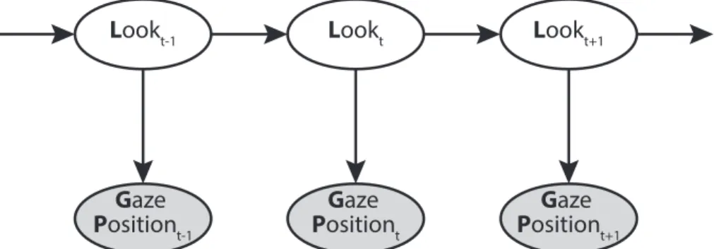
end of the clip), respectively. Figure 5 shows a graphical representation of how the joint probability distribution factorizes in the HMM.
Equation 2 shows that in order to solve the HMM, we need to define a prior distribu-tion over looksP(L0), a transition model that expresses the probability of going from one look to another P(Lt|Lt−1), and a likelihood model for each possible look that determines the likelihood of an observed gaze position under that look P(GPt|Lt). In our model, we
consider seven different types of looks: 1. looking at ball A (A look), 2. looking at ball B (B look), 3. predicting where ball A will go (Predict A), 4. predicting where ball B will go (Predict B), 5. predicting where A would go if B wasn’t present in the scene (Counterfactual A), 6. predicting where B would go if ball A wasn’t present in the scene
Lookt-1 Lookt Lookt+1
Gaze
Positiont-1 PositionGaze t PositionGaze t+1
Figure 5. A graphical model representing a slice of the Hidden Markov Model. The value of variable Lookt only depends on the value of variable Lookt−1. The value of variable Lookt
(Counterfactual B), and 7. looking anywhere on the screen (Other). A gaze position
GP is defined by its x and y coordinates. For each type of look, we need to define a like-lihood function that specifies how likely different possible gaze positions are. We define the following likelihood functions for the four qualitatively different kinds of looks (looking, predicting,counterfactual,other).
The likelihood that a given gaze position GP at timet was alook at ball Bis
P(GPt|Lt= looking,B)∝exp(−
d(Bt, GPt)
2σ2 ), (3)
where d(Bt, GPt) refers to the Euclidian distance between the location of ball B and gaze
positionGP at timet. We fixed the varianceσ2 to be 30 pixels for all likelihood functions. Note that Bcan either refer to ball A or ballB, depending on what look we are interested in.
The likelihood that a given gaze positionGP at timetwas apredictive look of where ball B will be is P(GPt|Lt= predicting,B)∝ T X i=t+1 γe−γ(i−t)·exp(−d(Bi, GPt) 2σ2 ), (4) where we sum over the Euclidian distances between the current gaze position GPt and all
future positions of ball Bt+1:T. We discount future positions by an exponential function
with rate parameter γ. For predictive looks, we fix γ = 0.1. This means that future ball positions that are closer in time to the current position of the ball are more likely than ball positions later in the future.
The likelihood that a given gaze position GP at time t was a counterfactual look of where ballB would go if the other ball was not present in the scene is
P(GPt|Lt= counterfactual,B)∝ T X i=t0 γe−γ(i−t)·exp(−d(B 0 i, GPt) 2σ2 ), (5) where we sum over the Euclidian distances between the current gaze position GPt and all
future positions that the ball would have hadB0t0:T in the counterfactual situation in which the other ball was removed from the scene. Note that the time point t0 from which we consider where ball B would have been is defined as
t0 =
collision time, ift <collision time
t+ 1, otherwise.
most likely to be close to the point at which the two balls would have collided. This is where the actual world and the counterfactual world part ways. After the time at which the two balls collided, a counterfactual look is most likely when a gaze position is close to where the ball would have been at this time in point. For counterfactual looks, we fix γ = 0.05. This means that compared to predictive looks, future gaze positions are discounted somewhat less.
Finally, we define the likelihood that a given gaze positionGP at timetwas an “other look” as
P(GPt|Lt= other)∝
1
max(x)max(y) (6)
where max(x) andmax(y) refer to the maximum dimensions of the video with 1000 pixels and 750 pixels, respectively.
Now that we have likelihood functions for each kind of lookP(GPt|Lt), we still need
to determine the prior distributionP(L0), as well as the transition model P(Lt|Lt−1). For the prior, we simply consider a uniform distribution over the different types of looks. To determine the transition model, we ran a separate HMM for each participant and learned the transition model via the EM algorithm (Dempster et al., 1977).
For our analysis, we considered two quantities: First, we were interested in the pos-terior marginal distribution over looks P(Lt|GP1:T) at each time point. Figure ?? shows
the average posterior marginal distribution by condition. Second, we were interested in de-termining the most likely sequence of looks for each participant and clip. We implemented the Viterbi algorithm to do so (Forney Jr, 1973). The clips in the supplementary materials show the most likely state that participants are in at any given point in time at the top.