Reducing multiclass to binary: A unifying approach for margin classifiers

Reducing Multiclass to Binary:

A Unifying Approach for Margin Classifiers

Erin L. Allwein [email protected]

Southwest Research Institute 6220 Culebra Road

San Antonio, TX 78228

Robert E. Schapire [email protected]

AT&T Labs;Research

Shannon Laboratory

180 Park Avenue, Room A203 Florham Park, NJ 07932

Yoram Singer [email protected]

School of Computer Science & Engineering Hebrew University, Jerusalem 91904, Israel

Editor: Leslie Pack Kaelbling

Abstract

We present a unifying framework for studying the solution of multiclass categorization prob-lems by reducing them to multiple binary probprob-lems that are then solved using a margin-based binary learning algorithm. The proposed framework unifies some of the most popular approaches in which each class is compared against all others, or in which all pairs of classes are compared to each other, or in which output codes with error-correcting properties are used. We propose a general method for combining the classifiers generated on the binary problems, and we prove a general empirical multiclass loss bound given the empirical loss of the individual binary learning algorithms. The scheme and the corresponding bounds apply to many popular classification learn-ing algorithms includlearn-ing support-vector machines, AdaBoost, regression, logistic regression and decision-tree algorithms. We also give a multiclass generalization error analysis for general output codes with AdaBoost as the binary learner. Experimental results with SVM and AdaBoost show that our scheme provides a viable alternative to the most commonly used multiclass algorithms.

1. Introduction

Many supervised machine learning tasks can be cast as the problem of assigning elements to a finite set of classes or categories. For example, the goal of optical character recognition (OCR) systems is to determine the digit value (

0

;:::;

9

) from its image. The number of applications that require multiclass categorization is immense. A few examples for such applications are text and speech categorization, natural language processing tasks such as part-of-speech tagging, and gesture and object recognition in machine vision.

In designing machine learning algorithms, it is often easier first to devise algorithms for dis-tinguishing between only two classes. Some machine learning algorithms, such as C4.5 (Quinlan, 1993) and CART (Breiman, Friedman, Olshen, & Stone, 1984), can then be naturally extended to handle the multiclass case. For other algorithms, such as AdaBoost (Freund & Schapire, 1997;

Schapire & Singer, 1999) and the support-vector machines (SVM) algorithm (Vapnik, 1995; Cortes & Vapnik, 1995), a direct extension to the multiclass case may be problematic. Typically, in such cases, the multiclass problem is reduced to multiple binary classification problems that can be solved separately. Connectionist models (Rumelhart, Hinton, & Williams, 1986), in which each class is represented by an output neuron, are a notable example: each output neuron serves as a discrimina-tor between the class it represents and all of the other classes. Thus, this training algorithm is based on a reduction of the multiclass problem to

k

binary problems, where

k

is the number of classes.

There are many ways to reduce a multiclass problem to multiple binary classification problems. In the simple approach mentioned above, each class is compared to all others. Hastie and Tibshi-rani (1998) suggest a different approach in which all pairs of classes are compared to each other. Dietterich and Bakiri (1995) presented a general framework in which the classes are partitioned into opposing subsets using error-correcting codes. For all of these methods, after the binary classifi-cation problems have been solved, the resulting set of binary classifiers must then be combined in some way. In this paper, we study a general framework, which is a simple extension of Dietterich and Bakiri’s framework, that unifies all of these methods of reducing a multiclass problem to a binary problem.

We pay particular attention to the case in which the binary learning algorithm is one that is based on the margin of a training example. Roughly speaking, the margin of a training example is a number that is positive if and only if the example is correctly classified by a given classifier and whose magnitude is a measure of confidence in the prediction. Several well known algorithms work directly with margins. For instance, the SVM algorithm (Vapnik, 1995; Cortes & Vapnik, 1995) at-tempts to maximize the minimum margin of any training example. There are many more algorithms that attempt to minimize some loss function of the margin. AdaBoost (Freund & Schapire, 1997; Schapire & Singer, 1999) is one example: it can be shown that AdaBoost is a greedy procedure for minimizing an exponential loss function of the margins. In Section 2, we catalog many other algo-rithms that also can be viewed as margin-based learning algoalgo-rithms, including regression, logistic regression and decision-tree algorithms.

The simplest method of combining the binary classifiers (which we call Hamming decoding) ignores the loss function that was used during training as well as the confidences attached to pre-dictions made by the classifier. In Section 3, we give a new and general technique for combining classifiers that does not suffer from either of these defects. We call this method loss-based decoding. We next prove some of the theoretical properties of these methods in Section 4. In particular, for both of the decoding methods, we prove general bounds on the training error on the multiclass problem in terms of the empirical performance on the individual binary problems. These bounds indicate that loss-based decoding is superior to Hamming decoding. Also, these bounds depend on the manner in which the multiclass problem has been reduced to binary problems. For the one-against-all approach, our bounds are linear in the number of classes, but for a reduction based on random partitions of the classes, the bounds are independent of the number of classes. These results generalize more specialized bounds proved by Schapire and Singer (1999) and by Guruswami and Sahai (1999).

In Section 5, we prove a bound on the generalization error of our method when the binary learner is AdaBoost. In particular, we generalize the analysis of Schapire et al. (1998), expressing a bound on the generalization error in terms of the training-set margins of the combined multiclass classifier, and showing that boosting, when used in this way, tends to aggressively increase the margins of the training examples.

Finally, in Section 6, we present experiments using SVM and AdaBoost with a variety of multiclass-to-binary reductions. These results show that, as predicted by our theory, loss-based decoding is almost always better than Hamming decoding. Further, the results show that the most commonly used one-against-all reduction is easy to beat, but that the best method seems to be problem-dependent.

2. Margin-based Learning Algorithms

We study methods for handling multiclass problems using a general class of binary algorithms that attempt to minimize a margin-based loss function. In this section, we describe that class of learning algorithms with several examples.

A binary margin-based learning algorithm takes as input binary labeled training examples

(

x

1

;y

1

)

;:::;

(

x

m

;y

m

)

where the instances

x

i

belong to some domain

X and the labels

y

i

2 f;

1

;

+1

g. Such a learning algorithm uses the data to generate a real-valued function or

hypoth-esis

f

:

X ! R where

f

belongs to some hypothesis spaceF. The margin of an example

(

x;y

)

with respect to

f

is

yf

(

x

)

. Note that the margin is positive if and only if the sign of

f

(

x

)

agrees with

y

. Thus, if we interpret the sign of

f

(

x

)

as its prediction on

x

, then

1

m

m

X

i

=1

[[

y

i

f

(

x

i

)

0]]

is exactly the training error of

f

, where, in this case, we count a zero output (

f

(

x

i

) = 0

) as a mistake. (Here and throughout this paper,

[[

]]

is

1

if predicate

holds and

0

otherwise.)

Although minimization of the training error may be a worthwhile goal, in its most general form the problem is intractable (see for instance the work of H¨offgen and Simon (1992)). It is therefore often advantageous to instead minimize some other nonnegative loss function of the margin, that is, to minimize

1

m

m

X

i

=1

L

(

y

i

f

(

x

i

))

(1)

for some loss function

L

:

R !

[0

;

1

)

. Different choices of the loss function

L

and different

algorithms for (approximately) minimizing Eq. (1) over some hypothesis space lead to various well-studied learning algorithms. Below we list several examples. In the present work, we are not particularly concerned with the method used to achieve a small empirical loss since we will use these algorithms later in the paper as “black boxes.” We focus instead on the loss function itself whose properties will allow us to prove our main theorem on the effectiveness of output coding methods for multiclass problems.

Support-vector Machines. For training data that may not be linearly separable, the support-vector machines (SVM) algorithm (Vapnik, 1995; Cortes & Vapnik, 1995) seeks a linear classifier

f

:

R

n

!Rof the form

f

(

x

) =

wx

+

b

that minimizes the objective function

1

2

jjw jj 2 2

+

C

m

X

i

=1

i

;

for some parameter

C

, subject to the linear constraints

Put another way, the SVM solution forwis the minimizer of the regularized empirical loss function

1

2

jjw jj 2 2

+

C

m

X

i

=1

(1

;

y

i

((

w

x

i

) +

b

))

+

;

where

(

z

)

+

= max

f

z;

0

g. (For a more formal treatment see, for instance, the work of Sch¨olkopf et

al. (1998).) Although the role of the

L

2 norm of

w in the objective function is fundamental in

order for SVM to work, the analysis presented in the next section (and the corresponding multiclass algorithm) depends only on the loss function (which is a function of the margins). Thus, SVM can be viewed here as a binary margin-based learning algorithm which seeks to achieve small empirical risk for the loss function

L

(

z

) = (1

;

z

)

+

.

AdaBoost. The algorithm AdaBoost (Freund & Schapire, 1997; Schapire & Singer, 1999) builds a hypothesis

f

that is a linear combination of weak or base hypotheses

h

t

:

f

(

x

) =

X

t

t

h

t

(

x

)

:

The hypothesis

f

is built up in a series of rounds on each of which an

h

t

is selected by a weak or base learning algorithm and

t

2 Ris then chosen. It has been observed by Breiman (1997a,

1997b) and other authors (Collins, Schapire, & Singer, 2000; Friedman, Hastie, & Tibshirani, 2000; Mason, Baxter, Bartlett, & Frean, 1999; R¨atsch, Onoda, & M¨uller, to appear; Schapire & Singer, 1999) that the

h

t

’s and

t

’s are effectively being greedily chosen so as to minimize

1

m

m

X

i

=1

e

;

y

i

f

(

x

i )

:

Thus, AdaBoost is a binary margin-based learning algorithm in which the loss function is

L

(

z

) =

e

;

z

.

AdaBoost with randomized predictions. In a little studied variant of AdaBoost (Freund & Schapire, 1997), we allow AdaBoost to output randomized predictions in which the predicted label of a new example

x

is chosen randomly to be

+1

with probability

1

=

(1 +

e

;2

f

(

x

)

)

. The loss suffered then is the probability that the randomly chosen predicted label disagrees with the correct label

y

. Let

p

(

x

)

def

= 1

=

(1 +

e

;2

f

(

x

)

)

. Then the loss is

p

(

x

)

if

y

=

;

1

and

1

;

p

(

x

)

if

y

= +1

. Using a simple

algebraic manipulation, the loss can be shown to be

1

=

(1+

e

2

yf

(

x

)

)

. So for this variant of AdaBoost, we set

L

(

z

) = 1

=

(1 +

e

2

z

)

. However, in this case, note that the learning algorithm is not directly attempting to minimize this loss (it is instead minimizing the exponential loss described above). Regression. There are various algorithms, such as neural networks and least squares regression, that attempt to minimize the squared error loss function

(

y

;

f

(

x

))

2

. When the

y

’s are inf;

1

;

+1

g,

this function can be rewritten as

(

y

;

f

(

x

))

2

=

y

2

(

y

;

f

(

x

))

2

= (

yy

;

yf

(

x

))

2

= (1

;

yf

(

x

))

2

:

Thus, for binary problems, minimizing squared error fits our framework where

L

(

z

) = (1

;

z

)

2

Logistic regression. In logistic regression and related methods such as Iterative Scaling (Csisz´ar & Tusn´ady, 1984; Della Pietra, Della Pietra, & Lafferty, 1997; Lafferty, 1999), and LogitBoost (Fried-man et al., 2000), one posits a logistic model for estimating the conditional probability of a positive label:

Pr [

y

= +1

j

x

] =

1

1 +

e

;2

f

(

x

)

:

One then attempts to maximize the likelihood of the labels in the sample, or equivalently, to mini-mize the log loss

;

log(Pr [

y

j

x

]) = log(1 +

e

;2

yf

(

x

)

)

:

Thus, for logistic regression and related methods, we take

L

(

z

) = log(1 +

e

;2

z

)

.

Decision trees. The most popular decision tree algorithms can also be naturally linked to loss functions. For instance, Quinlan’s C4.5 (1993), in its simplest form, for binary classification prob-lems, splits decision nodes in a manner to greedily minimize

X leaf

j

p

+

j

ln

p

;

j

+

p

+

j

p

+

j

!

+

p

;

j

ln

p

;

j

+

p

+

j

p

;

j

!! (2) where

p

+

j

and

p

;

j

are the fraction of positive and negative examples reaching leaf

j

, respectively. The prediction at leaf

j

is then

sign(

p

+

j

;

p

;

j

)

. Viewed differently, imagine a decision tree that instead outputs a real number

f

j

at each leaf with the intention of performing logistic regression as above. Then the empirical loss associated with logistic regression is

X leaf

j

p

+

j

ln(1 +

e

;2

f

j

) +

p

;

j

ln(1 +

e

2

f

j

)

:

This is minimized, over choices of

f

j

, when

f

j

= (1

=

2)ln(

p

+

j

=p

;

j

)

. Plugging in this choice gives exactly Eq. (2), and thresholding

f

j

gives the hard prediction rule used earlier. Thus, C4.5, in this simple form, can be viewed as a margin-based learning algorithm that is naturally linked to the loss function used in logistic regression.

By similar reasoning, CART (Breiman et al., 1984), which splits using the Gini index, can be linked to the square loss function, while Kearns and Mansour’s (1996) splitting rule can be linked to the exponential loss used by AdaBoost.

The analysis we present in the next section might also hold for other algorithms that tacitly employ a function of the margin. For instance, Freund’s BrownBoost algorithm (1999) implicitly uses an instance potential function that satisfies the condition we impose on

L

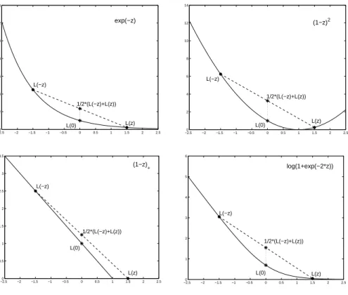
. Therefore, it can also be combined with output coding and used to solve multiclass problems. To conclude this section, we plot in Figure 1 some of the loss functions discussed above.

3. Output Coding for Multiclass Problems

In the last section, we discussed margin-based algorithms for learning binary problems. Suppose now that we are faced with a multiclass learning problem in which each label

y

is chosen from a set

Yof cardinality

k >

2

. How can a binary margin-based learning algorithm be modified to handle a

k

-class problem?

−2.50 −2 −1.5 −1 −0.5 0 0.5 1 1.5 2 2.5 2 4 6 8 10 12 14 L(−z) L(z) 1/2*(L(−z)+L(z)) L(0) exp(−z) −2.50 −2 −1.5 −1 −0.5 0 0.5 1 1.5 2 2.5 2 4 6 8 10 12 14 L(−z) L(z) 1/2*(L(−z)+L(z)) L(0) (1−z)2 −2.50 −2 −1.5 −1 −0.5 0 0.5 1 1.5 2 2.5 0.5 1 1.5 2 2.5 3 3.5 L(−z) L(z) 1/2*(L(−z)+L(z)) L(0) (1−z) + −2.50 −2 −1.5 −1 −0.5 0 0.5 1 1.5 2 2.5 1 2 3 4 5 6 L(−z) L(z) 1/2*(L(−z)+L(z)) L(0) log(1+exp(−2*z))

Figure 1: Some of the margin-based loss functions discussed in the paper: the exponential loss used by AdaBoost (top left); the square loss used in least-squares regression (top right); the “hinge” loss used by support-vector machines (bottom left); and the logistic loss used in logistic regression (bottom right).

Several solutions have been proposed for this question. Many involve reducing the multiclass problem, in one way or another, to a set of binary problems. For instance, perhaps the simplest approach is to create one binary problem for each of the

k

classes. That is, for each

r

2 Y, we

apply the given margin-based learning algorithm to a binary problem in which all examples labeled

y

=

r

are considered positive examples and all other examples are considered negative examples. We then end up with

k

hypotheses that somehow must be combined. We call this the one-against-all approach.

Another approach, suggested by Hastie and Tibshirani (1998), is to use the given binary learning algorithm to distinguish each pair of classes. Thus, for each distinct pair

r

1

;r

2

2 Y, we run the

learning algorithm on a binary problem in which examples labeled

y

=

r

1are considered positive,

and those labeled

y

=

r

2 are negative. All other examples are simply ignored. Again, the

;

k

2

hypotheses that are generated by this process must then be combined. We call this the all-pairs approach.

A more general suggestion on handling multiclass problems was given by Dietterich and Bakiri (1995). Their idea is to associate each class

r

2Y with a row of a “coding matrix”M2f;

1

;

+1

g

k

`

for some

`

. The binary learning algorithm is then run once for each column of the matrix on the induced binary problem in which the label of each example labeled

y

is mapped to

M

(

y;s

)

. This yields

`

hypotheses

f

s

. Given an example

x

, we then predict the label

y

for which row

y

of matrixMis

“closest” to

(

f

1

(

x

)

;:::;f

`

(

x

))

. This is the method of error correcting output codes (ECOC).

In this section, we propose a unifying generalization of all three of these methods applica-ble to any margin-based learning algorithm. This generalization is closest to the ECOC approach of Dietterich and Bakiri (1995) but differs in that the coding matrix is taken from the larger set

f;

1

;

0

;

+1

g

k

`

. That is, some of the entries

M

(

r;s

)

may be zero, indicating that we don’t care how hypothesis

f

s

categorizes examples with label

r

.

Thus, our scheme for learning multiclass problems using a binary margin-based learning algo-rithmAworks as follows. We begin with a given coding matrix

M2f;

1

;

0

;

+1

g

k

`

:

For

s

= 1

;:::;`

, the learning algorithmAis provided with labeled data of the form

(

x

i

;M

(

y

i

;s

))

for all examples

i

in the training set but omitting all examples for which

M

(

y

i

;s

) = 0

. The algorithmAuses this data to generate a hypothesis

f

s

:

X !R.

For example, for the one-against-all approach,Mis a

k

k

matrix in which all diagonal elements

are

+1

and all other elements are;

1

. For the all-pairs approach, Mis a

k

;

k

2

matrix in which each column corresponds to a distinct pair

(

r

1

;r

2

)

. For this column,

Mhas

+1

in row

r

1,

;

1

in

row

r

2and zeros in all other rows.

As an alternative to callingArepeatedly, in some cases, we may instead wish to add the column

index

s

as a distinguished attribute of the instances received byA, and then learn a single hypothesis

on this larger learning problem rather than

`

hypotheses on smaller problems. That is, we provide

Awith instances of the form

((

x

i

;s

)

;M

(

y

i

;s

))

for all training examples

i

and all columns

s

for

which

M

(

y

i

;s

)

6

= 0

. AlgorithmA then produces a single hypothesis

f

:

X f

1

;:::;`

g ! R.

However, for consistency with the preceding approach, we define

f

s

(

x

)

to be

f

(

x;s

)

. We call these two approaches in whichAis called repeatedly or only once the multi-call and single-call variants,

respectively.

We note in passing that there are no fundamental differences between the single and multi-call variants. Most previous work on output coding employed the multi-call variant due to its simplicity. The single-call variant becomes handy when an implementation of a classification learning algo-rithm that outputs a single hypothesis of the form

f

:

Xf

1

;::: ;`

g!Ris available. We describe

experiments with both variants in Section 6.

For either variant, the algorithmAattempts to minimize the loss

L

on the induced binary

prob-lem(s). Recall that

L

is a function of the margin of an example so the loss of

f

s

on an example

x

i

with induced label

M

(

y

i

;s

)

2 f;

1

;

+1

gis

L

(

M

(

y

i

;s

)

f

s

(

x

i

))

. When

M

(

y

i

;s

) = 0

, we want to

entirely ignore the hypothesis

f

s

in computing the loss. We can define the loss to be any constant in this case, so, for convenience, we choose the loss to be

L

(0)

so that the loss associated with

f

s

on example

i

is

L

(

M

(

y

i

;s

)

f

s

(

x

i

))

in all cases.

Thus, the average loss over all choices of

s

and all examples

i

is

1

m`

m

X

i

=1

`

X

s

=1

L

(

M

(

y

i

;s

)

f

s

(

x

i

))

:

(3)

We call this the average binary loss of the hypotheses

f

s

on the given training set with respect to coding matrix M and loss

L

. It is the quantity that the calls to Ahave the implicit intention of

minimizing. We will see in the next section how this quantity relates to the misclassification error of the final classifier that we build on the original multiclass training set.

LetM

(

r

)

denote row

r

of

M

and letf

(

x

)

be the vector of predictions on an instance

x

: f

(

x

) = (

f

1

(

x

)

;:::;f

`

(

x

))

:

Given the predictions of the

f

s

’s on a test point

x

, which of the

k

labels inY should be predicted?

While several methods of combining the

f

s

’s can be devised, in this paper, we focus on two that are very simple to implement and for which we can analyze the empirical risk of the original multiclass problem. The basic idea of both methods is to predict with the label

r

whose rowM

(

r

)

is “closest”

to the predictionsf

(

x

)

. In other words, predict the label

r

that minimizes

d

(

M

(

r

)

;

f

(

x

))

for some

distance

d

. This formulation begs the question, however, of how we measure distance between the two vectors.

One way of doing this is to count up the number of positions

s

in which the sign of the prediction

f

s

(

x

)

differs from the matrix entry

M

(

r;s

)

. Formally, this means our distance measure is

d

H

(

M

(

r

)

;

f

(

x

)) =

`

X

s

=1

1

;

sign(

M

(

r;s

)

f

s

(

x

))

2

(4) where

sign(

z

)

is

+1

if

z >

0

, ;

1

if

z <

0

, and

0

if

z

= 0

. This is essentially like computing

Hamming distance between row M

(

r

)

and the signs of the

f

s

(

x

)

’s. However, note that if either

M

(

r;s

)

or

f

s

(

x

)

is zero then that component contributes

1

=

2

to the sum. For an instance

x

and a matrix

M

, the predicted label

y

^

2f

1

;:::;k

gis therefore

^

y

= arg min

_r

d

H

(

M

(

r

)

;

f

(

x

))

:

We call this method of combining the

f

s

’s Hamming decoding.

A disadvantage of this method is that it ignores entirely the magnitude of the predictions which can often be an indication of a level of “confidence.” Our second method for combining predictions takes this potentially useful information into account, as well as the relevant loss function

L

which is ignored with Hamming decoding. The idea is to choose the label

r

that is most consistent with the predictions

f

s

(

x

)

in the sense that, if example

x

were labeled

r

, the total loss on example

(

x;r

)

would be minimized over choices of

r

2Y. Formally, this means that our distance measure is the

total loss on a proposed example

(

x;r

)

:

d

L

(

M

(

r

)

;

f

(

x

)) =

`

X

s

=1

L

(

M

(

r;s

)

f

s

(

x

))

:

(5)

Analogous to Hamming decoding, the predicted label

y

^

2f

1

;::: ;k

gis

^

y

= arg min

_r

d

L

(

M

(

r

)

;

f

(

x

))

:

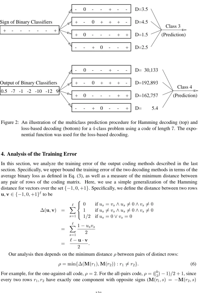
We call this approach loss-based decoding. An illustration of the two decoding methods is given in Figure 2. The figure shows the decoding process for a problem with

4

classes using an output code of length

`

= 7

. For clarity we denote in the figure the entries of the output code matrix by

+

,;and

0

(instead of

+1

,;

1

and

0

). Note that in the example, the predicted class of the loss-based decoding

(which, in this case, uses exponential loss) is different than that of the Hamming decoding.

We note in passing that the loss-based decoding method for log-loss is the well known and widely used maximum-likelihood decoding which was studied briefly in the context of ECOC by Guruswami and Sahai (1999).

Class 3 (Prediction) -+ - - + - -- + + + + - - - + + -+ -+ - - - +

Sign of Binary Classifiers

0 D=3.5 0 D=4.5 + 0 D=1.5 0 D=2.5 -+ - - + - -- + + + + - - - + + + -+ -Output of Binary Classifiers

(Prediction) Class 4 0 0 0 0 0.5 -7 -1 -2 -10 -12 9 D= 30,133 D=192,893 D=162,757 D= 5.4

Figure 2: An illustration of the multiclass prediction procedure for Hamming decoding (top) and loss-based decoding (bottom) for a

4

-class problem using a code of length

7

. The expo-nential function was used for the loss-based decoding.

4. Analysis of the Training Error

In this section, we analyze the training error of the output coding methods described in the last section. Specifically, we upper bound the training error of the two decoding methods in terms of the average binary loss as defined in Eq. (3), as well as a measure of the minimum distance between any pair of rows of the coding matrix. Here, we use a simple generalization of the Hamming distance for vectors over the setf;

1

;

0

;

+1

g. Specifically, we define the distance between two rows u

;

v2f;

1

;

0

;

+1

g

`

to be

(

u

;

v

) =

`

X

s

=1 8 > < > :

0

if

u

s

=

v

s

^

u

s

6

= 0

^

v

s

6

= 0

1

if

u

s

6

=

v

s

^

u

s

6

= 0

^

v

s

6

= 0

1

=

2

if

u

s

= 0

_

v

s

= 0

=

X

`

s

=1

1

;

u

s

v

s

2

=

`

;uv

2

:

Our analysis then depends on the minimum distance

between pairs of distinct rows:

= min

f

(

M

(

r

1

)

;

M

(

r

2

)) :

r

1 6

=

r

2 g

:

(6)

For example, for the one-against-all code,

= 2

. For the all-pairs code,

= (

;

k

2

;

1)

=

2 + 1

, since

every two rows

r

1

;r

2 have exactly one component with opposite signs (

M

(

r

1

;s

) =

;M

(

r

and M

(

r

1

;s

)

6

= 0

) and for the rest at least one component of the two is

0

(M

(

r

1

;s

) = 0

or

M

(

r

2

;s

) = 0

). For a random matrix with components chosen uniformly over either

f;

1

;

+1

gor

f;

1

;

0

;

+1

g, the expected value of

(

M

(

r

1

)

;

M

(

r

2

))

for any distinct pair of rows is exactly

`=

2

.

Intuitively, the larger

, the more likely it is that decoding will “correct” for errors made by individual hypotheses. This was Dietterich and Bakiri’s (1995) insight in suggesting the use of output codes with error-correcting properties. This intuition is reflected in our analysis in which a larger value of

gives a better upper bound on the training error. In particular, Theorem 1 states that the training error is at most

`=

times worse than the average binary loss of the combined hypotheses (after scaling the loss by

L

(0)

). For the one-against-all matrix,

`=

=

`=

2 =

k=

2

which can be large if the number of classes is large. On the other hand, for the all-pairs matrix or for a random matrix,

`=

is close to the constant

2

, independent of

k

.

We begin with an analysis of loss-based decoding. An analysis of Hamming decoding will follow as a corollary. Concerning the loss

L

, our analysis assumes only that

L

(

z

) +

L

(

;

z

)

2

L

(0)

>

0

(7)

for all

z

2 R. Note that this property holds if

L

is convex, although convexity is by no means a

necessary condition. Note also that all of the loss functions in Section 2 satisfy this property. The property is illustrated in Figure 1 for four of the loss functions discussed in that section.

Theorem 1 Let

"

be the average binary loss (as defined in Eq. (3)) of hypotheses

f

1

;:::;f

`

on a

given training set

(

x

1

;y

1

)

;:::;

(

x

m

;y

m

)

with respect to the coding matrix

M 2 f;

1

;

0

;

+1

g

k

`

and loss

L

, where

k

is the cardinality of the label set Y. Let

be as in Eq. (6). Assume that

L

satisfies Eq. (7) for all

z

2R. Then the training error using loss-based decoding is at most

`"

L

(0)

:

Proof: Suppose that loss-based decoding incorrectly classifies an example

(

x;y

)

. Then there is some label

r

6

=

y

for which

d

L

(

M

(

r

)

;

f

(

x

))

d

L

(

M

(

y

)

;

f

(

x

))

:

(8)

Let

S

=

f

s

:

M

(

r;s

)

6

=

M

(

y;s

)

^

M

(

r;s

)

6

= 0

^

M

(

y;s

)

6

= 0

g

be the set of columns ofMin which rows

r

and

y

differ and are both non-zero. Let

S

0

=

f

s

:

M

(

r;s

) = 0

_

M

(

y;s

) = 0

g

be the set of columns in which either row

r

or row

y

is zero. Let

z

s

=

M

(

y;s

)

f

s

(

x

)

and

z

0

s

=

M

(

r;s

)

f

s

(

x

)

. Then Eq. (8) becomes

`

X

s

=1

L

(

z

0

s

)

`

X

s

=1

L

(

z

s

)

which implies X

s

2

S

[

S

0

L

(

z

0

s

)

X

s

2

S

[

S

0

L

(

z

s

)

since

z

s

=

z

0

s

if

s

62

S

[

S

0. This in turn implies that

`

X

s

=1

L

(

z

s

)

X

s

2

S

[

S

0

L

(

z

s

)

1

2

X

s

2

S

[

S

0

(

L

(

z

0

s

) +

L

(

z

s

))

= 12

X

s

2

S

(

L

(

z

0

s

) +

L

(

z

s

))

+12

X

s

2

S

0

(

L

(

z

0

s

) +

L

(

z

s

))

:

(9) If

s

2

S

then

z

0

s

=

;

z

s

and, by assumption,

(

L

(

;

z

s

) +

L

(

z

s

))

=

2

L

(0)

. Thus, the first term

of Eq. (9) is at least

L

(0)

j

S

j. If

s

2

S

0, then either

z

s

= 0

or

z

0

s

= 0

. Either case implies that

L

(

z

0

s

) +

L

(

z

s

)

L

(0)

. Thus, the second term of Eq. (9) is at last

L

(0)

j

S

0

j

=

2

.

Therefore, Eq. (9) is at least

L

(0)

j

S

j

+

j

S

0 j

2

=

L

(0)(

M

(

r

)

;

M

(

y

))

L

(0)

:

In other words, a mistake on training example

(

x

i

;y

i

)

implies that

`

X

s

=1

L

(

M

(

y

i

;s

)

f

s

(

x

i

))

L

(0)

so the number of training mistakes is at most

1

L

(0)

m

X

i

=1

`

X

s

=1

L

(

M

(

y

i

;s

)

f

s

(

x

i

)) =

_L

m`"

₍₀₎

and the training error is at most

`"=

(

L

(0))

as claimed.

As a corollary, we can give a similar but weaker theorem for Hamming decoding. Note that we use a different assumption about the loss function

L

, but one that also holds for all of the loss functions described in Section 2.

Corollary 2 Let

f

1

;:::;f

`

be a set of hypotheses on a training set

(

x

1

;y

1

)

;:::;

(

x

m

;y

m

)

, and let

M2 f;

1

;

0

;

+1

g

k

`

be a coding matrix where

k

is the cardinality of the label setY. Let

be as

in Eq. (6). Then the training error using Hamming decoding is at most

1

m

m

X

i

=1

`

X

s

=1

(1

;

sign(

M

(

y

i

;s

)

f

s

(

x

i

)))

:

(10)

Moreover, if

L

is a loss function satisfying

L

(

z

)

L

(0)

>

0

for

z <

0

and

"

is the average binary

loss with respect to this loss function, then the training error using Hamming decoding is at most

2

`"

Proof: Consider the loss function

H

(

z

) = (1

;

sign(

z

))

=

2

. From Eqs. (4) and (5), it is clear

that Hamming decoding is equivalent to loss-based decoding using this loss function. Moreover,

H

satisfies Eq. (7) for all

z

so we can apply Theorem 1 to get an upper bound on the training error of

2

m

m

X

i

=1

`

X

s

=1

H

(

M

(

y

i

;s

)

f

s

(

x

i

))

(12)

which equals Eq. (10).

For the second part, note that if

z

0

then

H

(

z

)

1

L

(

z

)

=L

(0)

, and if

z >

0

then

H

(

z

) = 0

L

(

z

)

=L

(0)

. This implies that Eq. (12) is bounded above by Eq. (11).

Theorem 1 and Corollary 2 are broad generalizations of similar results proved by Schapire and Singer (1999) in a much more specialized setting involving only AdaBoost. Also, Corollary 2 generalizes some of the results of Guruswami and Sahai (1999) that bound the multiclass training error in terms of the training (misclassification) error rates of the binary classifiers.

The bounds of Theorem 1 and Corollary 2 depend implicitly on the fraction of zero entries in the matrix. Intuitively, the more zeros there are, the more examples that are ignored and the harder it should be to drive down the training error. At an extreme, ifMis all zeros, then

is fairly large

(

`=

2

) but learning certainly should not be possible. To make this dependence explicit, let

T

=

f

(

i;s

) :

M

(

y

i

;s

) = 0

g

be the set of pairs

i;s

inducing examples that are ignored during learning. Let

q

=

j

T

j

=

(

m`

)

be the

fraction of ignored pairs. Let

"

be the average binary loss restricted to the pairs not ignored during training:

"

= 1

j

T

c

j X (

i;s

)2

T

c

L

(

M

(

y

i

;s

)

f

s

(

x

i

))

where

T

c

=

f

(

i;s

) :

M

(

y

i

;s

)

6

= 0

g. Then the bound in Theorem 1 can be rewritten

`

L

(0)

m`

1

0 @ X (

i;s

)2

T

L

(0) +

X (

i;s

)62

T

L

(

M

(

y

i

;s

)

f

s

(

x

i

))

1 A

=

`

q

+ (1

;

q

)

"

L

(0)

:

Similarly, let

be the fraction of misclassification errors made on

T

c

:

= 1

j

T

c

j X (

i;s

)2

T

c

[[

M

(

y

i

;s

)

6

= sign(

f

s

(

x

i

))]]

:

The first part of Corollary 2 implies that the training error using Hamming decoding is bounded above by

`

(

q

+ 2(1

;

q

)

)

:

We see from these bounds that there are many trade-offs in the design of the coding matrixM.

On the one hand, we want the rows to be far apart so that

will be large, and we also want there to be few non-zero entries so that

q

will be small. On the other hand, attempting to make

large and

q

small may produce binary problems that are difficult to learn, yielding large (restricted) average binary loss.

5. Analysis of Generalization Error for Boosting with Loss-based Decoding

The previous section considered only the training error using output codes. In this section, we take up the more difficult task of analyzing the generalization error. Because of the difficulty of obtaining such results, we do not have the kind of general results obtained for training error which apply to a broad class of loss functions. Instead, we focus only on the generalization error of using AdaBoost with output coding and loss-based decoding. Specifically, we show how the margin-theoretic analysis of Schapire et al. (1998) can be extended to this more complicated algorithm.

Briefly, Schapire et al.’s analysis was proposed as a means of explaining the empirically ob-served tendency of AdaBoost to resist overfitting. Their theory was based on the notion of an example’s margin which, informally, measures the “confidence” in the prediction made by a classi-fier on that example. They then gave a two-part analysis of AdaBoost: First, they proved a bound on the generalization error in terms of the margins of the training examples, a bound that is indepen-dent of the number of base hypotheses combined, and a bound suggesting that larger margins imply lower generalization error. In the second part of their analysis, they proved that AdaBoost tends to aggressively increase the margins of the training examples.

In this section, we give counterparts of these two parts of their analysis for the combination of AdaBoost with loss-based decoding. We also assume that the single-call variant is used as described in Section 3. The result is essentially the AdaBoost.MO algorithm of Schapire and Singer (1999) (specifically, what they called “Variant 2”).

This algorithm works as follows. We assume that a coding matrixMis given. The algorithm

works in rounds, repeatedly calling the base learning algorithm to obtain a base hypothesis. On each round

t

= 1

;:::;T

, the algorithm computes a distribution

D

t

over pairs of training examples and columns of the matrixM, i.e., over the setf

1

;:::;m

gLwhereL

=

f

1

;:::;`

g. The base learning

algorithm uses the training data (with binary labels as encoded usingM) and the distribution

D

t

to

obtain a base hypothesis

h

t

:

X L! f;

1

;

+1

g. (In general,

h

t

’s range may beR, but here, for

simplicity, we assume that

h

t

is binary valued.) The error

t

of

h

t

is the probability with respect to

D

t

of misclassifying one of the examples. That is,

t

= Pr

(

i;s

)

D

t

[

M

(

y

i

;s

)

6

=

h

t

(

x

i

;s

)]

=

X

m

i

=1

`

X

s

=1

D

t

(

i;s

)[[

M

(

y

i

;s

)

6

=

h

t

(

x

i

;s

)]]

:

The distribution

D

t

is then updated using the rule

D

t

+1

(

i;s

) =

D

t

(

i;s

)exp(

;

t

M

(

y

i

;s

)

h

t

(

x

i

;s

))

Z

t

:

(13)

Here,

t

= (1

=

2)ln((1

;

t

)

=

t

)

(which is nonnegative, assuming, as we do, that

t

1

=

2

), and

Z

t

is a normalization constant ensuring that

D

t

+1is a distribution. It is straightforward to show that

Z

t

= 2

q

t

(1

;

t

)

:

(14)

(The initial distribution is chosen to be uniform so that

D

1

(

i;s

) = 1

=

(

m`

)

.)

After

T

rounds, this procedure outputs a final classifier

H

which, because we are using loss-based decoding, is

H

(

x

) = arg min

_y

2Y

`

X

s

=1

exp

;

M

(

y;s

)

T

X

t

=1

t

h

t

(

x;s

)

!

:

(15)

We begin our margin-theoretic analysis with a definition of the margin of this combined multi-class multi-classifier. First, let

(

f;;x;y

) =

;

1

ln

1

`

`

X

s

=1

e

;

M

(

y;s

)

f

(

x;s

) !

:

If we let

=

X

T

t

=1

t

;

(16) and

f

(

x;s

) = 1

X

T

t

=1

t

h

t

(

x;s

)

;

(17)

we can then rewrite Eq. (15) as

H

(

x

) = arg max

_y

2Y

(

f;;x;y

)

:

(18)

Since we have transformed the argument of the minimum in Eq. (15) by a strictly decreasing func-tion (namely,

x

7! ;

(1

=

)ln(

x=`

)

) to arrive at Eq. (18) it is clear that we have not changed the

definition of

H

. This rewriting has the effect of normalizing the argument of the maximum in Eq. (18) so that it is always in the range

[

;

1

;

+1]

. We can now define the margin for a labeled

example

(

x;y

)

to be the difference between the vote

(

f;;x;y

)

given to the correct label

y

, and the largest vote given to any other label. We denote the margin byM

f;

(

x;y

)

. Formally,

M

f;

(

x;y

) = 12

(

f;;x;y

)

;

max

r

6=

y

(

f;;x;r

)

;

where the factor of

1

=

2

simply ensures that the margin is in the range

[

;

1

;

+1]

. Note that the margin

is positive if and only if

H

correctly classifies example

(

x;y

)

.

Although this definition of margin is seemingly very different from the one given earlier in the paper for binary problems (which is the same as the one used by Schapire et al. in their compar-atively simple context), we show next that maximizing training-example margins translates into a better bound on generalization error, independent of the number of rounds of boosting.

Let Hbe the base-hypothesis space of f;

1

;

+1

g-valued functions on X L. We let

co(

H

)

denote the convex hull ofH:

co(

H

) =

(

f

:

x

7! X

h

h

h

(

x

)

j

h

0

;

X

h

h

= 1

)

;

where it is understood that each of the sums above is over the finite subset of hypotheses inHfor

which

h

>

0

. Thus,

f

as defined in Eq. (17) belongs to

co(

H

)

.

We assume that training examples are chosen i.i.d. from some distribution Don X Y. We

write probability or expectation with respect to a random choice of an example

(

x;y

)

according to

Das

Pr

D

[

]

and

E

D

[

]

. Similarly, probability and expectation with respect to an example chosen

uniformly at random from training set

S

is denoted

Pr

S

[

]

and

E

S

[

]

.

We can now prove the first main theorem of this section which shows how the generalization error can be usefully bounded when most of the training examples have large margin. This is very similar to the results of Schapire et al. (1998) except for the fact that it applies to loss-based decoding for a general coding matrixM.

Theorem 3 Let D be a distribution over

X

Y, and let

S

be a sample of

m

examples chosen

independently at random according toD. Suppose the base-classifier spaceHhas VC-dimension

d

, and let

>

0

. Assume that

m

d`

1

where

`

is the number of columns in the coding matrix

M. Then with probability at least

1

;

over the random choice of the training set

S

, every weighted

average function

f

2

co(

H

)

and every

>

0

satisfies the following bound for all

>

0

:

Pr

D

[

M

f;

(

x;y

)

0]

Pr

S

[

M

f;

(

x;y

)

] +

O

0 @

1

p

m

d

log

2

(

`m=d

)

2

+ log(1

=

)

! 1

=

2 1 A

:

Proof: To prove the theorem, we will first need to define the notion of a sloppy cover, slightly specialized for our purposes. For a class F of real-valued functions over X Y, a training set

S

X Y of size

m

, and real numbers

>

0

and

0

, we say that a function class

^

F is an

-sloppy

-cover of F with respect to

S

if, for all

F

in F, there exists

F

^

in F

^

with

Pr

S

h

j

F

^

(

x;y

)

;

F

(

x;y

)

j

>

i

. Let N

(

F

;;;m

)

denote the maximum, over all training

sets

S

of size

m

, of the size of the smallest

-sloppy

-cover ofF with respect to

S

.

Using techniques from Bartlett (1998), Schapire et al. (1998, Theorem 4) give a theorem which states that, for

>

0

and

>

0

, the probability over the random choice of training set

S

that there exists any function

F

2F for which

Pr

D

[

F

(

x;y

)

0]

>

Pr

S

[

F

(

x;y

)

] +

is at most

2

N

(

F

;=

2

;=

8

;

2

m

)

e

;

2

m=

32

:

(19) We prove Theorem 3 by applying this result to the family of functions

F

=

fM

f;

:

f

2

co(

H

)

; >

0

g

:

To do so, we need to construct a relatively small set of functions that approximate all the functions inF.

We start with a lemma that implies that any functionM

f;

can be approximated by M

f;

^

for some

^

in the small finite set

E

=

ln

`

i

:

i

= 1

;:::;

ln

`

2

2

:

Lemma 4 For all

>

0

, there exists

^

2E

such that for all

f

2

co(

H

)

and for all

x

2X,

r

2Y,

Proof: Let

(

;

z

) = 1

ln

1

`

`

X

s

=1

e

z

s !

forz2R

`

. We claim first that, for anyz, and for

0

<

1

2,

0

(

2

;

z

)

;

(

1

;

z

)

1

1 ;

1

2

ln

`:

(20)

For the first inequality, it suffices to show that

F

(

) = (

;

z

)

is nondecreasing. Differentiating,

we find that

dF

d

= ln

`

+

P

`s

=1

p

s

ln

p

s

2 (21) where

p

s

=

e

z

s

=

P

`s

=1

e

z

s. Since entropy over

`

symbols cannot exceed

ln

`

, this quantity is

nonnegative.

For the second inequality of Eq. (20), it suffices to show that

G

(

) = (

;

z

) + (ln

`

)

=

is

nonincreasing. Again differentiating (or reusing Eq. (21)), we find that

dG

d

=

P

`s

=1

p

s

ln

p

s

2

which is nonpositive since entropy cannot be negative.

So, if

min

E

, then let

^

= (ln

`

)

=

(

i

)

be the largest element ofE

that is no bigger than

.

If

i >

1

then

ln

`

i

<

ln

`

(

i

;

1)

so

0

(

;

z

)

;

(^

;

z

)

i

ln

`

;

1

ln

`

i

ln

`

;

(

i

;

1)

ln

`

ln

`

=

:

If

i

= 1

, then

0

(

;

z

)

;

(^

;

z

)

ln

`

;

1

ln

`

:

It remains then only to handle the case that

is small. Assume thatz2

[

;

1

;

+1]

`

. Then

(

;

z

) = 1

ln

1

`

`

X

s

=1

e

z

s !

1

ln

exp

2

2 +

`

`

X

s

=1

z

s

!!

=

_{2 +}

1

_`

X

`

s

=1

z

s

:

This is because, as proved by Hoeffding (1963), for any random variable

X

with

a

X

b

, and for

>

0

,

E

h

e

X

i

exp

2

(

b

;

a

)

2

8

+

E [

X

]

!

:

On the other hand, by Eq. (20),

(

;

z

)

lim

!0

(

;

z

)

= lim

!0 1

`

P

`s

=1

e

z

s

z

s

1

`

P

`s

=1

e

z

s

= 1

_`

X

`

s

=1

z

s

where the first equality uses l’Hˆopital’s rule. Thus, if

<

min

E

, then we take

^

= min

E

2

so that

1

`

`

X

s

=1

z

s

(

;

z

)

(^

;

z

)

1

`

`

X

s

=1

z

s

+ ^

₂

which implies that

j

(

;

z

)

;

(^

;

z

)

j

^

2

assumingz 2

[

;

1

;

+1]

`

. Since

(

f;;x;r

) =

;

(

;

z

)

with

z

s

=

;

M

(

r;s

)

f

(

x;s

)

2

[

;

1

;

+1]

,

this completes the lemma.

Let

S

be a fixed subset of X Y of size

m

. Because Hhas VC-dimension

d

, there exists a

subsetH

^

ofHof cardinality

(

e`m=d

)

d

that includes all behaviors on

S

. That is, for all

h

2 H,

there exists

^

h

2H

^

such that

h

(

x;s

) = ^

h

(

x;s

)

for all

(

x;y

)

2

S

and all

s

2L. Now let

C

N

=

(

f

: (

x;s

)

7!

1

N

N

X

i

=1

h

i

(

x;s

)

j

h

i

2H

^

)

be the set of unweighted averages of

N

elements inH

^

, and let

^

F

N;

=

fM

f;

:

f

2C

N

;

2E

g

:

We will show thatF

^

N;

is a sloppy cover ofF.

Let

f

2

co(

H

)

. Then we can write

f

(

x;s

) =

X

j

j

h

j

(

x;s

)

where

j

0

and

P

j

j

= 1

. Because we are only interested in the behavior of

f

on points in

S

, we can assume without loss of generality that each

h

j

2H

^

.

Lemma 5 Suppose for some

x

2X and some

g

2C

N

, we have thatj

f

(

x;s

)

;

g

(

x;s

)

j

for all

s

2L. Let

>

0

and let

^

2E

be as in Lemma 4. Then for all

y

2Y,

j M

f;

(

x;y

)

;M

g;

^

Proof: For all

r

2Y,

(

f;;x;r

)

;

(

g;;x;r

) = 1

ln

P

s

exp(

;

M

(

r;s

)

g

(

x;s

))

P

s

exp(

;

M

(

r;s

)

f

(

x;s

))

1

ln

max

_s

exp(

;

M

(

r;s

)(

g

(

x;s

)

;

f

(

x;s

)))

= max

_s

M

(

r;s

)(

f

(

x;s

)

;

g

(

x;s

))

max

s

j

M

(

r;s

)

jj

f

(

x;s

)

;

g

(

x;s

)

j

where the first inequality uses the simple fact that

(

P

i

a

i

)

=

(

P

i

b

i

)

max

i

a

i

=b

i

for positive

a

i

’s

and

b

i

’s. By the symmetry of this argument,

j

(

f;;x;r

)

;

(

g;;x;r

)

j

:

Also, from Lemma 4,

j

(

g;;x;r

)

;

(

g;

;x;r

^

)

j

so

j

(

f;;x;r

)

;

(

g;

;x;r

^

)

j

2

for all

r

2Y. By definition of margin, this implies the lemma.

Recall that the coefficients

j

are nonnegative and that they sum to one; in other words, they define a probability distribution overH

^

. It will be useful to imagine sampling from this distribution.

Specifically, suppose that

^

h

2 H

^

is chosen in this manner. Then for fixed

(

x;s

)

,

^

h

(

x;s

)

is a f;

1

;

+1

g-valued random variable with expected value of exactly

f

(

x;s

)

. Consider now choosing

N

such functions

h

^

1

;:::;

^

h

N

independently at random, each according to this same distribution, and

let

g

= (1

=N

)

P

Ni

=1

^

h

i

. Then

g

2C

N

. Let us denote byQthe resulting distribution over functions

inC

N

. Note that, for fixed

(

x;s

)

,

g

(

x;s

)

is the average of

N

f;

1

;

+1

g-trials with expected value

f

(

x;s

)

.

For any

(

x;y

)

2

S

,

Pr

g

Q

[

j M

f;

(

x;y

)

;M

g;

^

(

x;y

)

j

>

2

]

Pr

g

Q

[

9

s

2L

:

j

f

(

x;s

)

;

g

(

x;s

)

j

>

]

`

X

s

=1

Pr

g

Q

[

j

f

(

x;s

)

;

g

(

x;s

)

j

>

]

2

`e

;

N

2

=

2

:

These three inequalities follow, respectively, from Lemma 5, the union bound and Hoeffding’s inequality. Thus,

E

g

Q

[Pr

S

[

jM

f;

(

x;y

)

;M

g;

^

(

x;y

)

j

>

2

]]

= E

S

[Pr

g

Q

[

j M

f;

(

x;y

)

;M

g;

^

(

x;y

)

j

>

2

]]

2

`e

;

N

2

=

2

:

Therefore, there exists

g

2C

N

such that

Pr

S

[

jM

f;

(

x;y

)

;M

g;

^

(

x;y

)

j

>

2

]

2

`e

;

N

2

=

2

:

We have thus shown thatF

^

N;

is a

2

`e

;

N

2

=

2

-sloppy

2

-cover ofF. In other words,

N

(

F

;

2

;

2

`e

;

N

2

=

2

;m

)

jF

^

N;

j

e`m

d

dN

ln

`

2

2

:

Making the appropriate substitutions, this gives that Eq. (19) is at most

16ln

`

2

2

e`m

d

(32

d=

2 )ln(16

`=

)

e

;

m

2

=

32

:

(22) Let

= 16

0 @

ln

16ln

l

2

8

m

+ 2

m

d

2

ln

2

e`m

d

ln

e`

2

m

d

! 1 A 1

=

2

:

Note that the quantity inside the square root is at least

2

d=

(

m

2

)

d=

(

me

)

. Thus,

16

p

d=

(

me

)

.

Using this approximation for the first occurrence of

, it follows that Eq. (22) is at most

.

We have thus proved the bound of the theorem for a single given choice of

>

0

with high probability. To prove that the bound holds simultaneously for all

>

0

, we can use exactly the same argument used by Schapire and Singer (1999) in the very last part of their Theorem 8.

Thus, we have shown that large training-set margins imply a better bound on the generalization error, independent of the number of rounds of boosting. We turn now to the second part of our analysis in which we prove that AdaBoost.MO tends to increase the margins of the training exam-ples, assuming that the binary errors

t

of the base hypotheses are bounded away from the trivial error rate of

1

=

2

(see the discussion that follows the proof). The theorem that we prove below is a direct analog of Theorem 5 of Schapire et al. (1998) for binary AdaBoost. Note that we focus only on coding matrices that do not contain zeros. A slightly weaker result can be proved in the more general case.

Theorem 6 Suppose the base learning algorithm, when called by AdaBoost.MO using coding

ma-trixM2f;

1

;

+1

g

k

`

, generates hypotheses with weighted binary training errors

1

;:::;

T

. Let

be as in Eq. (6). Then for any

0

, we have that

Pr

S

[

M

f;

(

x;y

)

]

`

T

Y

t

=1

2

q

1;

t

(1

;

t

)

1+

where

f

and

are as in Eqs. (16) and (17).

Proof: Suppose, for some labeled example

(

x;y

)

,M

f;

(

x;y

)

. Then, by definition of margin,

there exists a label

r

2Y;f

y

gfor which

1

2(

(

f;;x;y

)

;

(

f;;x;r

))

;

that is

`

X

s

=1

e

;

M

(

r;s

)

f

(

x;s

)

e

2

`

X

s

=1

e

;

M

(

y;s

)

f

(

x;s

)

:

(23)

Let

z

s

=

M

(

y;s

)

f

(

x;s

)

;

and

z

0

s

=

M

(

r;s

)

f

(

x;s

) +

. Let

S

=

f

s

2L

:

M

(

r;s

)

6

=

M

(

y;s

)

g. Then Eq. (23) implies

`

X

s

=1

e

;

z

s

`

X

s

=1

e

;

z

0 s and so

`

X

s

=1

e

;

z

s

`

X

s

=1

e

;

z

s

+

e

;

z

0 s

2

X

s

2

S

e

;

z

s

+

e

;

z

0 s

2

=

X

s

2

S

e

;

z

s

+

e

z

s

2

j

S

j

:

This is because, if

s

2

S

then

z

0

s

=

;

z

s

, and because

x

+ 1

=x

2

for all

x >

0

.

Therefore, ifM

f;

(

x;y

)

then

`

X

s

=1

e

;

M

(

y;s

)

f

(

x;s

)

e

;

:

Thus, the fraction of training examples

i

for whichM

f;

(

x

i

;y

i

)

is at most

e

m

m

X

i

=1

`

X

s

=1

e

;

M

(

y

i

;s

)

f

(

x

i

;s

)

=

`e

X

m

i

=1

`

X

s

=1

1

m`

exp

;

T

X

t

=1

t

M

(

y

i

;s

)

h

t

(

x

i

;s

)

! (24)

=

`e

X

m

i

=1

`

X

s

=1

T

Y

t

=1

Z

t

!

D

T

+1

(

i;s

)

(25)

=

`e

Y

T

t

=1

Z

t

!

:

(26)

Here, Eq. (24) uses the definition of

f

and

as in Eqs. (16) and (17). Eq. (25) uses the definition of

D

T

+1as defined recursively in Eq. (13). Eq. (26) uses the fact that

D

T

+1 is a distribution. The

theorem now follows by plugging in Eq. (14) and applying straightforward algebra.

As noted by Schapire et al. (1998), this bound can be usefully understood if we assume that

t

1

=

2

;

for all

t

. Then the upper bound simplifies to

`

q

(1

;

2

)

1;

(1 + 2

)

1+

T

:

If

<

, then the expression inside the parentheses is smaller than one so that the fraction of