An Improved Method for Spectroscopic Quality Classification

(1)

University of New Mexico University of New Mexico

UNM Digital Repository

Mathematics & Statistics ETDs Electronic Theses and Dissertations

Summer 7-8-2020

An Improved Method for Spectroscopic Quality Classification

Elizabeth G. Mayer

Follow this and additional works at: https://digitalrepository.unm.edu/math_etds

Part of the Applied Mathematics Commons, Mathematics Commons, Psychiatry and Psychology Commons, and the Statistics and Probability Commons

Recommended Citation Recommended Citation

Mayer, Elizabeth G.. "An Improved Method for Spectroscopic Quality Classification." (2020). https://digitalrepository.unm.edu/math_etds/151

This Thesis is brought to you for free and open access by the Electronic Theses and Dissertations at UNM Digital Repository. It has been accepted for inclusion in Mathematics & Statistics ETDs by an authorized administrator of UNM Digital Repository. For more information, please contact [email protected], [email protected], [email protected].

(2)

Candidate Department

This dissertation is approved, and it is acceptable in quality and form for publication: Approved by the Dissertation Committee:

, Chairperson

Elizabeth Grace Mayer

Mathematics & Statistics

Dr. Erik Erdhardt

Dr. Fletcher Christensen

Dr. Rhoshel Lenroot

(3)

An Improved Method for Spectroscopic

Quality Classification

by

Elizabeth Grace Mayer

B.S., UNM, 2017

M.S., UNM, 2020

THESIS

Submitted in Partial Fulfillment of the Requirements for the Degree of

Master of Science

Statistics

The University of New Mexico Albuquerque, New Mexico

(4)

(5)

Dedication

To all the faculty at the University of New Mexico’s Statistics department who helped. To Dr. Bustillo and Dr. Lenroot for the funding and data. To my family and friends for never giving up on me.

(6)

Acknowledgments

Dr. Erik Erhardt, for being my adviser and for extensive help with the coding of this analysis.

Dr. Rhoshel Lenroot, for being a member of my committee and for funding my Master’s.

Dr. Fletcher Christensen, for being a member of my committee. Dr. Juan Bustillo, for the data set and for funding my Master’s. Linda Mayer, for proofreading the thesis extensively.

(7)

An Improved Method for Spectroscopic

Quality Classification

by

Elizabeth Grace Mayer

B.S., UNM, 2017

M.S., UNM, 2020

M.S., Statistics, University of New Mexico, 2020

Abstract

Spectral quality classification is a vital step in data cleaning before the analysis of magnetic resonance spectroscopy (MRS) data can be done. This analysis compares five methods of quality classification; three of these are legacy methods, Maudsley et al. (2006), Zhang et al. (2018), and Bustillo et al. (2020), and two newly created methods that used a random forests classifier (RFC) to inform their classifications. We found that the random forest classifier was the most accurate at predicting spectra quality (balanced accuracy for RF of 88% vs legacy of 70%, 72%, or 72%). A Random-Forests-Informed Filtering method (RFIFM) for quality classification was created by bounding four of the highest ranking features in the RFC to mimic the classification methods of the legacy methodologies. The RFIFM had only slightly decreased accuracy compared to the RFC (85% vs 88%), but still outclassed the legacy methods. Overall, the top features in the RFC show that the best measures of quality relate to the frequency of the metabolite peaks in the spectra.

(8)

List of Figures

1.1 Axial brain slice of a control brain with labeled features. Note the image is in neurological format (right side of brain on right), with the frontal lobe facing up. . . 4 1.2 Differences between suppressed (A) and unsuppressed (A) spectra.

The x-axis measures the chemical shift of the spectra in ppm. The y-axis shows the strength of the signal. Because of the strength of the water signal in A the two figures have different scaling of their y-axis with A being the original scale and B being 500x closer. Figure from Befroy and Shulman (2011). . . 5 1.3 Poor quality and good quality spectra with metabolite labels. Notice

that the poor-quality spectrum has a large water peak artifact at 4 ppm, the lack of large metabolite peaks found in the good-quality spectrum, and generally a larger variance in the baseline noise. . . . 10 1.4 An NAA peak, which is an identifiable hill in the spectrum associated

with a metabolite, with labeled features. The shaded region is the NAA Area. . . 12

2.1 Spectral quality classification guide used by experts to rate the spec-tra in the spec-training set. . . 25 2.2 An example decision tree for our analysis with the features of a

(13)

2.3 Details of how to calculate the each statistical measures in Sec-tion 2.7.1 using a confusion matrix. . . 35

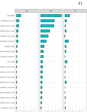
3.1 Plots mapping the VIMP ranking of each feature in the RFC. 0 = Poor Quality, 1 = Good Quality . . . 41 3.2 Receiver operating characteristic (ROC) curve for the RFC with the

optimal threshold, which is the proportion of trees that need to clas-sify the spectrum as “good” for the forests to clasclas-sify the spectrum as “good”. . . 42 3.3 These plots map out the likelihood of a voxel being of “good”

qual-ity based on the specified feature value on the y-axis and the feature values on the x-axis. The blue line is a Loess curve for the points in the plot. The orange bars represent the acceptable boundaries being used in for each feature in the RFIFM. Please note these bound-aries are not optimized and we acknowledge the poor bounds for CR frequency. . . 44 3.4 Plot of the confusion matrix values. See Section 2.7.1 for explanation

of each statistical measure. . . 47 3.5 Case 1: Plot of 5 random spectra classified as “good” by both the

legacy and random-forest-informed methods. . . 48 3.6 Case 2: Plot of 5 random spectra classified as “poor” by both the

legacy and random-forest-informed methods. . . 49 3.7 Case 3: Plot of 5 random spectra classified as “good” by the

random-forests-informed methods and “poor” by the legacy methods. . . 49 3.8 Case 4: Plot of 5 random spectra classified as “good” by the legacy

methods and “poor” by the random-forests-informed methods. . . . 50 3.9 Plots comparing the proportion of subjects with quality data at a

(14)

3.10 MFM 100% subject inclusion brain map. . . 55

3.11 ZFM 100% subject inclusion brain map. . . 56

3.12 BFM 100% subject inclusion brain map. . . 57

3.13 RFC 100% subject inclusion brain map. . . 58

(15)

List of Tables

2.1 Inclusion Features with limits if Applicable. . . 23

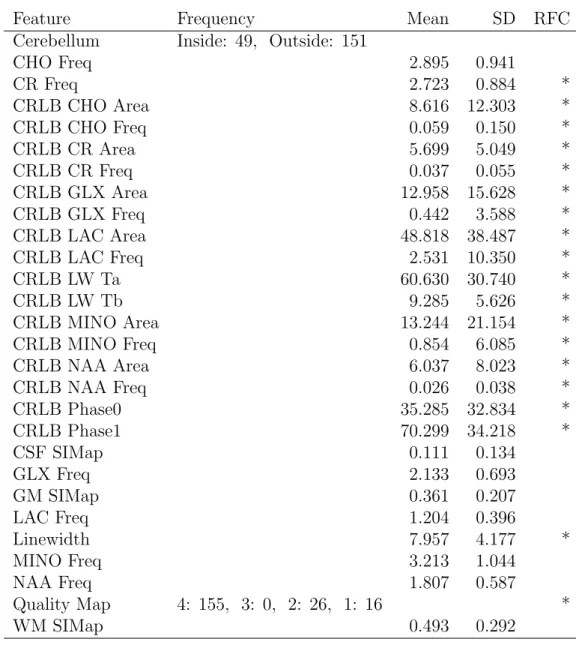
3.1 Demographics table of training set subjects. . . 38 3.2 Feature demographics for the two hundred voxels pulled for the

train-ing set. . . 39 3.3 Demographics table of application set subjects. . . 39 3.4 Lower and upper boundaries for each feature that were considered in

the RFIFM. . . 43 3.5 Confusion Matrix values. . . 46 3.6 The number of voxels based on the percentage of subjects with good

(16)

Chapter 1 Introduction

1.1 Magnetic Resonance Spectroscopy (MRS)

stud-ies the concentration of molecules in an object

Magnetic Resonance Spectroscopy (MRS) is a way of examining the concentration of nuclei within the body. It is an ionizing-radiation-free technique that is most often used to examine the metabolic changes of brain tumors, strokes, and seizures. Magnetic resonance (MR), a term coined by 1944 Nobel Prize winner Isidor Isaac Rabi who discovered the phenomena, is the process in which the protons in the body are aligned with a strong magnetic field, then these protons “flip” when a radio wave is pulsed through a patient, throwing the protons out of equilibrium (Pfeifer, 1999; Rinck, 2008). Under normal circumstances nuclei are randomly oriented, but when a magnetic field acts on the nuclei they become oriented to the direction of the new field. The radio waves, a type of electromagnetic radiation, are then pulsed to create a secondary static magnetic field, referred to asβ0, perpendicular to the first one, which

causes the nuclei to spin out of equilibrium (Bl¨uml, 2013). The radio waves are then shut off and the protons return to equilibrium. These rates of change in the magnetic field as it returns to equilibrium are unique to the chemical nature of the molecules. Spectroscopy is when MR is used to determine the concentration of the individual

(17)

compounds in a region, which is plotted to create a spectrum of the frequencies being measured. MRS was first implemented in the 1940s and 50s independently by Edward Mills Purcell and Felix Bloch, who for their work jointly received the Nobel prize in Physics in 1952 (Pfeifer, 1999; Rinck, 2008). Their experiments later became the basis for imaging using MR. Later, in 2003, Professor Sir Peter Mansfield and Professor Paul Lauterbur worked on methodology to give MRS clinical applications, for which they were jointly awarded the Nobel Prize for Medicine (Rinck, 2008). MRS is applied clinically in one of two ways,in-vitro orin-vivo MRS. One of the fundamental issues with MRS acquisition is the low concentration of molecules relative to the large potential for noise, in-vitro or in-vivo MRS each handle this issue in a different manner.

1.1.1 In-vitro

Magnetic Resonance Spectroscopy

In-vitro MRS (Latin for “within the glass”) MRS is the older of the two methods, requiring a biopsy of tissue that can then be pulsed (outside of a living organism) with an incredibly strong magnetic field, usually 11.7–18.8 Teslas (T). The stronger the magnetic field the more accurate the spectrum and the better the resolution for more complex molecules, thus the issue of low concentrations of metabolites compared to the noise is removed. in-vitroMRS can tell us about selective parts of the brain tissue or more easily collected bodily fluids such as cerebral spinal fluid (CSF) (Khan et al., 2005; Cox et al., 2006). These areas where the biopsied brain tissue is collected are called regions of interest (ROI), which is a term used to describe a particular location in the brain that is of interest to a study. There is also evidence that brain chemistry changes rapidly after death, leading to inaccurate measures when compared to living tissue (Scheurer et al., 2005). Therefore, using the selective and invasive in-vitro

MRS, we have incredibly detailed knowledge of metabolic changes in brain tumors and the molecular brain composition of recently deceased patients. However, with this method, we are not given an understanding of how a living brain functions, both with and without illness.

(18)

1.1.2 In-vivo

Magnetic Resonance Spectroscopy

In-vivo (Latin for “within the living”) MRS is used in combination with Magnetic Resonance Imaging (MRI), to give a non-selective and non-invasive look into the molecular composition of the brain of a subject. Scans are done with a 3 T magnet, meaning compared to in-vitro MRS, the spectra are less accurate, especially for the more complex molecules in the brain (Bl¨uml, 2013).

First, the MRI measures the MR of just the hydrogen nuclei in the water of the molecules of the brain (Blüml, 2013). This creates incredibly accurate structural images in a very short period of time (under 10 minutes) called a T1-weighted image. The reason why the hydrogen nuclei in water can be used to create an accurate image of the brain is that the three tissue types in the brain, grey matter, white matter, and cerebral spinal fluid, have highly varied concentrations of water (Bandettini, 2012). Even though these measurements are from the hydrogen atom, individual nuclei are impossible to measure as their signal is too weak to register, so the signals are collected from a localized region, called a voxel (Blüml, 2013). For the MRI scans in this thesis, these localized regions are 1x1x1mm in size, though given the strength of the magnet and the complexity of the molecules being measured, the size of the localized region is subject to change (Blüml, 2013).

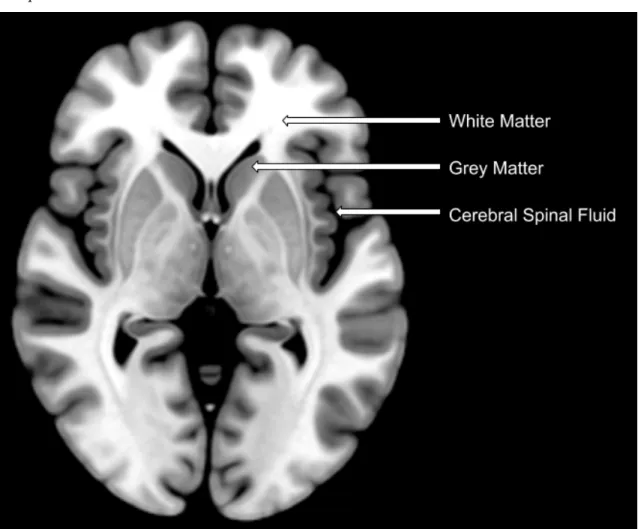
The grey matter (GM) areas of the brain are the areas of the brain dense with cell tissue and neurons (Bandettini, 2012). The GM structures are a much darker grey in our T1-weighted image (Figure 1.1). Whereas white matter (WM) are the connective tissue structures between the dense grey matter areas (Bandettini, 2012). In Figure 1.1, the WM structures are lighter in the image. The third tissue type in the T1-weighted image is the cerebral spinal fluid (CSF), which is not a tissue at all, but it is the fluid buffer between the brain and the skull and in interstitial regions that suspends the brain inside the head (Bandettini, 2012). Though, due to it’s high water concentration, CSF is also measured, but is of little interest because of its lack of brain tissue. The CSF is represented in the dark regions surrounding the brain and in the ventricles.

(19)

Figure 1.1: Axial brain slice of a control brain with labeled fea-tures. Note the image is in neurological format (right side of brain on right), with the frontal lobe facing up.

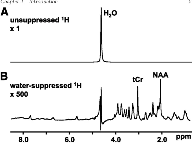
After the T1-weighted image, the magnetic resonance spectroscopy (MRS) scan is collected. This scan can take much longer (about 30 minutes or less depending on the kind of in-vivo analysis being done) and measures the hydrogen protons attached to other molecules in the brain (Bl¨uml, 2013). Due to their weak hydrogen atom signal, a specialized process must be used to pull these spectra that are unique to the study in which the molecules of interest are defined, these defined molecules are referred to as metabolites. For our study, we only measure six metabolites (N-Acetylaspartate, Creatine, Choline, Myo-inositol, and the combination of Glutamate and Glutamine), indicated as peaks or the defined hills whose height shows the strength of a molecule’s signal, in Figure 1.2 and in Figure 1.3.

(20)

Figure 1.2: Differences between suppressed (A) and unsuppressed (A) spectra. The x-axis measures the chemical shift of the spectra in ppm. The y-axis shows the strength of the signal. Because of the strength of the water signal in A the two figures have different scaling of their y-axis with A being the original scale and B being 500x closer. Figure from Befroy and Shulman (2011).

All MRS spectra use the same scale to measure the location of metabolites peaks. This scale is referred to as the chemical shift, which is measured in parts per million (ppm) of magnetic field. This universal scale is based on the location of the peak

of tetramethylsilane (TMS), a chemical solvent that was and still is added to

dissolved tissue samples in in-vitro MRS. This peak represents 0 on our horizontal axis and is used in in-vitro MRS to scale the spectra because it’s signal is a single identifiable peak, and all measurable molecules of interest appear to the left of its peak (Bl¨uml, 2013). A value on this scale measures the strength of the magnetic field required to produce resonance compared to TMS (Bl¨uml, 2013). For example, the peak labeled NAA in Figure 1.2B has a chemical shift of 2.0 ppm, meaning the

(21)

hydrogen atoms which created that peak require a magnetic field two millionths less than the field needed to produce resonance in TMS.

Despite not using TMS in in-vivo MRS the universal scale is still used so spec-tra from in-vivo and in-vitro spectra can be compared. In-vitro MRS studies have identified the chemical shift for all metabolites of interest, so in-vivo MRS uses this information and the location of a spectra’s water peak (typically at 4.7 ppm) to identify the location of each metabolite (Bl¨uml, 2013). For a labeled image of the peaks described below, see Figure 1.3.

As seen in Figure 1.2, N-Acetylaspartate (NAA), is the largest peak and is the second most abundant metabolite in the brain (Moffett et al., 2007). NAA is created by the mitochondria from aspacric acid and is often used as a neuronal marker for neuronal health in the brain (Moffett et al., 2007; Chatham and Blackband, 2001). This is due to finding NAA concentrations decreased in subjects suffering from nu-merous neurological conditions, such as Alzheimer’s disease or schizophrenia (Moffett et al., 2007; Chatham and Blackband, 2001). Creatine (CR) is the second simplest to measure metabolite and has the second largest peak in Figure 1.2 (tCR for total Creatine). This metabolite is found in the muscles and brains of vertebrates and facilitates the recycling of adenosine triphosphate (ATP) (Turner et al., 2015). Ge-netic deficiencies in the creatine pathway causes various severe neurological defects whose symptoms are intellectual disability and developmental delay (Turner et al., 2015). Choline (CHO) is an essential component in cell membranes and in the mem-branes of cell organelles (Erdman et al., 2012). Choline also produces acetylcholine, which is a neurotransmitter (Erdman et al., 2012). Myo-inositol (MINO), is a car-bocyclic sugar that mediates cell signal transduction (Parthasarathy et al., 2006). The final two metabolites of interest, Glutamate (GLU) and Glutamine (GLN), are too difficult to measure separately without a specialized process, so their signals are combined in most MRS studies as GLX (Bl¨uml, 2013). They are difficult to measure separately due to the high overlap of their peaks and the low amount of signal in each of these metabolites, which makes them not only difficult to discern from one another, but reduces the accuracy of measures for either metabolite when measuring

(22)

them independently (Bl¨uml, 2013). Despite GLU being the most abundant metabo-lite in the brain, GLU’s signal is incredibly weak. This excitatory neurotransmitter is responsible for sending signals between nerve cells and is also involved with energy metabolism (Goryawala et al., 2016). Because of these two uses interpretation of the concentrations of this metabolite are difficult. GLU is thought to be important for learning and memory, but in excess is thought to be toxic and to cause ailments such as Alzheimer’s disease (Hynd et al., 2004). In comparison, GLN is the precursor to many neurotransmitters including GLU (Goryawala et al., 2016). Problems in GLN metabolism and/or transport are associated with pathological conditions such as epilepsy (Goryawala et al., 2016).

Many approaches have been implemented to collectin-vivo MRS of which we are examining two: single-voxel spectroscopy (SVS) and whole-brain magnetic resonance spectroscopy (WB-MRSI). SVS examines a single ROI, similar to howin-vitro MRS used a biopsied region of the brain. Whole-brain spectroscopy focuses on scanning the entire brain and collecting the associated spectra. Below we will discuss the merits and function of both in-vivo MRS methodologies.

1.1.2.1 Single Voxel Spectroscopy (SVS)

SVS is the most commonly used MRS technique, due to its ease of use and for the immediate capacity to compare spectra (Zhang et al., 2018). SVS requires the investigator to pick an ROI that can be easily replicated in all subject brains, many SVS studies pull 2-6 ROIs. These ROIs each become a singular voxel in which all metabolite signals are combined to create a more accurate spectrum for the entire ROI (Bl¨uml, 2013). The ROI is defined as a specific anatomical location, such as the left insular cortex, that is common to all subjects. The ROI generally relates to a specific hypothesis. To reduce potential water-suppression issues, ROIs are in areas away from the sinuses or the corpus callosum, which are high in CSF (Bl¨uml, 2013). To measure this single ROI, scan times are about 1 to 3 minutes. This allows for much higher signal-to-noise ratio, that is, less noisy spectra, for the scanned ROIs.

(23)

Since SVS is similar to in-vitro spectroscopy studies, many of the same analysis methods and software used to analyze in-vitro studies apply also to SVS (Zhang et al., 2018).

The disadvantages of SVS are that you are trying to examine a complex system with an areas that are 4-8 cm3 _{in size (Bl¨}_{uml, 2013). For reference the human}

brain is approximately 1260 cm3, so we are examining 0.6% of the brain in the larger-volume studies with a single ROI (Cosgrove et al., 2007). We are essentially making assumptions about the structure of a newly discovered dinosaur with only bone fragments. The ROI approach means that we are excluding the other 99.4% of the brain for a single ROI that is easy to measure, which might have very little to do clinically with the diseases we are interested in studying.

1.1.2.2 Whole Brain spectroscopy (WB-MRSI)

Instead of choosing a single ROI, the brain is sliced into voxels, each of size 4.375x4.375x5.625 mm voxels, which is much larger than the T1-weighted image voxels (1mm3). These

larger voxels have been shown to have a large signal-to-noise ratio (SNR), compared to smaller voxel sizes, for the measured spectra (Zhang et al., 2018). However, these larger voxels have potentially lower SNR for their spectra when compared to SVS spectra. This allows for a non-selective analysis of the entire brain. Due to the increased magnitude of the number of voxels being examined, a single scan takes about 30 minutes with each voxel being scanned in a tenth of a second.

There are vast differences between subjects’ brain sizes and positions so an entire study must have each subject’s scan image warped into a group image space so that concentrations can be compared. This is unlike SVS, where because of the ROI approach, no further preprocessing is needed after collecting and processing the spectra of the ROI since the same region is being pulled for all subjects. Due to the analysis being done over the entire brain, statistical testing must take into account multiple comparisons over both voxels and metabolites (Zhang et al., 2018).

(24)

is amplified by the time frame of the WB-MRSI scan (Gurbani et al., 2018; Abdoli et al., 2016). Areas of the brain with abnormally high water and air concentrations (nasal cavities) cause issues in spectral measurement as they lead to potentially poor water signal suppression (Gurbani et al., 2018). Both can cause each spectrum to be non-representative of a voxel’s actual metabolite concentrations. Data cleaning is required before any sort of analysis can be done on the brain.

Due to technological leaps much of the preprocessing that was once impossible is now automated, but determining spectral quality is still a slow process. In a perfect world, a researcher would be able to examine each voxel in the whole brain, like SVS, and remove poorly-measured spectra to create an individualized mask per subject of only the highest quality voxels, mask being a binary collection of voxels in the brain with 1 meaning high quality and 0 meaning low quality. However, this is impossible due to the number of voxels in a WB-MRSI scan. So other measures of the spectra are used as measures of quality to automatically create these individualized subject masks. These masks are then combined to create a region of analysis in which all subjects have good quality data to run voxel-level statistical analyses, which are then combined to show clustered areas of regional differences in metabolite concentrations.

Since this approach is unspecified, WB-MRSI is not biased by previous findings in SVS studies. Instead of choosing an ROI where research has been extensively done, new areas of interest can be discovered. This leads to a better understanding of how a large portion of the brain’s internal chemistry changes in response to addiction, medication use, and illness, which is something SVS lacks. Instead of using a pin-hole to get a highly detailed view of a singular region, we have a wide angle shot of most of the brain, granted at a lower resolution, to examine.

(25)

Figure 1.3: Poor quality and good quality spectra with metabolite

labels. Notice that the poor-quality spectrum has a large water

peak artifact at 4 ppm, the lack of large metabolite peaks found in the good-quality spectrum, and generally a larger variance in the baseline noise.

1.2 The Importance of Spectral Quality Control

in

in-vivo

MRS

Poor-quality spectra (Figure 1.3, left) can distort our concentration measurements, which can lead to the appearance of a significant difference in metabolite concen-trations between two populations when there may not be any actual difference (or can mask a difference). These are spectra without identifiable metabolite peaks and can have a wavy baseline as seen in Figure 1.3 (left). In contrast, a high-quality spectrum is one in which all five metabolite peaks are identifiable and the baseline is level (does not drift up and down) (Figure 1.3 right). The baseline is an impor-tant reference since the concentration of the metabolite is determined by measuring the area between the spectrum’s estimated baseline and the metabolite peak. If the baseline curves drift greatly then the concentration could be overestimated or under-estimated. The same is true for identifying the peaks; if the preprocessing software has issues identifying a particular metabolite peak it might measure the wrong peak thus measuring an entirely unrelated metabolite, label a peak that isn’t there, or miss a peak altogether.

(26)

1.2.1 Current practices for Spectral Quality Control in SVS

SVS quality control is done by examining the individual spectrum for each subject. If the spectrum has unclear metabolite peaks or a largely curved baseline, then the subject is dropped from the analysis (Zhang et al., 2018; Bl¨uml, 2013). Essentially, the SVS quality control method is the gold standard for all other quality control methods.

1.2.2 Current practices for Spectral Quality Control in

WB-MRSI

1.2.2.1 Legacy Method: Filtering Specific Measures Using Bounds

WB-MRSI utilizes the filtering (selecting) of voxels based on two spectral measures as a determination of quality. These measures are the horizontal linewidth in hertz of the NAA peak and the Cram´er-Rao lower bound (CRLB) of the area under the peak of the individual metabolite. These two are detailed below. Figure 1.4 shows what each of these features are in relation to a spectrum.

The linewidth in hertz of the NAA peak at full width half max (FWHM), which is the full width of the peak at the halfway point between the baseline and peak, is used as an estimate of SNR. Because NAA is easy to measure, previous studies found that the quality of the spectra and its linewidth are correlated (Zhang et al., 2018; Pfeuffer et al., 1999; Bartha, 2007). Ideally, the linewidth is neither too narrow,<1 Hz, nor too wide, >16 Hz.

The use of the CRLB originated with SVS (Zhang et al., 2018), but has been co-opted by WB-MRSI. Essentially the CRLB measures the expected lower bound on the variance of the estimated concentration of a metabolite in a spectrum (Bolliger et al., 2013). CRLB and SNR are shown to be highly correlated (Bolliger et al., 2013). The CRLB of the area of a metabolite is used as a measure of the reliability of the calculated concentration for the quality measures (Zhang et al., 2018; Bolliger

(27)

2 ppm Frequency NAA Area Baseline Line width

Figure 1.4: An NAA peak, which is an identifiable hill in the spectrum associated with a metabolite, with labeled features. The shaded region is the NAA Area.

et al., 2013). So for this measure a CRLB >50 is considered too high, but a CRLB < 20 might be good. It is highly dependent on the ease of measurement of the metabolite (Bolliger et al., 2013).

While these three are used to measure quality in WB-MRSI, there is disagreement as to how each of these measures should be bound to best control for quality. Most studies differ slightly in how they filter for quality, though there are certainly agreed-upon limits. For example, in all studies a linewidth>16 is bad, but the upper bound for good quality lies between 10 and 13 hz for most studies (Pfeuffer et al., 1999;

(28)

Bartha, 2007). However, the upper bound for the quality metric is generally treated as the same for all metabolites.

1.2.2.2 Proposed Method: Supervised Machine Learning using a

Ran-dom Forests Classifier

If the ideal method for determining the quality of an individual spectrum is to have an expert examine the spectrum itself, then we wanted to create a method of spectra quality control that would most closely emulate this. Machine learning is defined as, “computer algorithms that improve automatically through experience” (Mitchell, 1997), with supervised machine learning being an algorithm trained on a data set that has been properly classified. Just like having an expert examining the individual spectrum, we wanted to train a machine learning classifier to identify quality spectra through training.

The Random Forests classifier (RFC) has repeatedly been shown to be one of the more accurate machine learning classification methods (Singh et al., 2016). We utilized its variable importance estimation, which measures the difference in classi-fication accuracy when a feature of the spectrum is included in the analysis versus when it is not (Louppe et al., 2013). The RFC utilizes a built-in external cross-validation classification error assessment, called out-of-bag error (Breiman, 2001).

For a detailed overview of the random forests method and associated background see Section 2.6.1.

1.3 Study Aims

Spectral quality classification is the basis of the WB-MRSI analysis framework. Aim 1 of this study is to examine three legacy methods of quality control filtering: the Maudsley et al. (2006), Zhang et al. (2018), and Bustillo et al. (2020) methodolo-gies. Each being a published WB-MRSI study with slightly different quality filters.

(29)

Aim 2 is to compare these legacy methods to a new method of quality determi-nation using a supervised machine learning random forests classifier.

Aim 3 is to create an easy-to-use filtering method informed by the random forests classifier. This filtering method will also be compared to the three legacy method-ologies and the random forests classifier.

(30)

Chapter 2 Methods

2.1 Study Design

A cross-sectional analysis was done to compare several methods of quality classifi-cation of WB-MRSI spectra. The quality classificlassifi-cation methods being examined are (Aim 1) Maudsley et al. (2006) (MFM), Zhang et al. (2018) (ZFM), Bustillo et al. (2020) (BFM), (Aim 2) the new Random Forests Classifier (RFC), and (Aim 3) the new Random-Forests-Informed Filtering method (RFIFM).

All methods were compared to each other with an examination of the accuracy, sensitivity, specificity, and other statistics of each method with a training set of 197 spectra rated by multiple experts. They were also compared by contrasting the fil-tered maps, which are three-dimensional matrices in which every voxel in a subject’s scan is represented by a single value, of ten randomly-selected control subjects re-ferred to as our application set. All of this was done so some measure of success can be prescribed to each method of quality classification.

(31)

2.2 Setting and Participants

All subjects underwent a magnetic resonance (MR) scan at 3T using a TIM Trio scanner at the Mind Research Network facility in Albuquerque, New Mexico, between the years of 2014 and 2018. Both patient (first episode psychosis, FEP) and healthy volunteer (HV) subjects were from the Bustillo et al. (2020) pilot study. All subjects in the study were recruited from the local Albuquerque population.

FEP were recruited from the University of New Mexico (UNM) Hospitals. Inclu-sion criteria were:

1. DSM-5 schizophrenia, schizophreniform, or bipolar disorder (SCID-DSM-5). 2. Age 16–40.

3. No current substance use disorder (except for nicotine). HV recruited from the community were included if they had:

1. No current DSM-5 disorder. 2. Age 16–40.

3. No history of neurological disorder.

4. No first-degree relatives with any psychotic disorder. 5. No current substance use disorder (except for nicotine).

The study was approved by the UNM Institutional Review Board. Subjects gave written informed consent and were reimbursed for their participation.

2.2.1 Training set for Random Forests Classifier and

Classi-fier Statistical Analysis

Twenty subjects (11 FEP, 9 HV) were sampled from the Bustillo et al. (2020) pilot study. For each subject, 10 WB-MRSI voxels were sampled uniformly along the longitudinal axis (z-direction) at an interval of roughly one voxel for each 3 z-plane slices. The x and y positions were picked using a random number generator limited

(32)

by the numbers of brain voxels in both the x and y axis. Of the 200 collected voxels, 197 voxels fell inside the brain; the training set consisted of the spectra for these 197 voxels. This is due to sampling voxels based on the T1-weighted image rather then the spectroscopic image, which exclude voxels in the out layers of the brain. This data set was used to train the RFC and to collect statistical measures for each of the classification methods.

2.2.2 Application set for Qualitative Assessment

For this analysis, 10 randomly sampled HVs from the total sample of 29 were used. This data set was being used to see how each classification method worked on actual data and to figure out of difficult the newer methods would be to set up.

2.3 Features of Spectra and Surrounding Tissue

There are twenty-eight (28) measures of a voxel’s spectrum that are being used as features of interest, and these reduce to eleven (11) groups due to feature repetition for each metabolite. The features used in each method of spectral quality classifica-tion are listed in Table 2.1. Below are descripclassifica-tions of each of these features. Please note that a star (*) next to a feature’s name means the variable is metabolite spe-cific, therefore there are five measures of that feature, one for each metabolite. See Figure 1.4 in Chapter 1.

Cerebellum A factor variable of whether or not the voxel lies within the

cere-bellum. The cerebellum has been shown to have spectra with higher CR peaks compared to NAA peaks which is generally not seen elsewhere in the brain. See Figure 1.3 in Section 1.2.

Cram´er-Rao Lower Bound of the Area* An important issue with MRS

(33)

in neighboring metabolites, making the quantification of the individual metabo-lite’s proportion in an individual spectrum difficult as multiple metabolites could have overlapping areas, which biases metabolite concentration estimates (Bolliger et al., 2013; Kreis, 2016). In order to properly group metabolites in a spectrum optimal measuring parameters (such as area, frequency, line shape parameters, and phase corrections) for the individual spectrum are calculated (Bolliger et al., 2013; Maudsley, 2005). The MIDAS program calculates Cram´er-Rao minimum variance bounds, or Cram´er-Rao lower bounds (CRLB) (Maudsley, 2005), which is the expected lower bound of variance for a collection of potential measuring parameters, and for each potential value for the measuring parameters. Then the value with the lowest expected variation is selected for each measuring parameter for the spectrum (Bolliger et al., 2013). Some of these measuring parameters are metabolite-specific (such as frequency and area), whereas others are spectrum-specific (such as phase corrections and line shape parameters).

The CRLB are calculated in the following manner using the Fisher matrix, formu-las from Iqbal et al. (2017):

F = Re(β×β 0₎ ˆ

σ2 . (2.1)

β represents the basis matrix, which is a vectorization of the spectra in the basis set. The basis set corresponds to the prior-knowledge of the location of each metabolite in the frequency domain. This prior-knowledge comes from in-vitro

MRS studies. β is the vectorization of the actual spectra being collected. The multiplication of the complex β vectors give us an N ×N covariance matrix, of which we take the real part (Re). ˆσ2 _{is an estimate of the noise variance in the}

spectrum.

The Fisher matrix is then used to create the CRLB:

CRLB=pdiag(F−1₎_. _(2.2)

Which means the diagonal element of the inverse of the Fisher matrix is taken. The relative CRLB, the values being used for this paper and that are being referenced every time CRLB is being called, is created by taking the CRLB and dividing by

(34)

the corresponding optimal measuring parameter (OMP below), then multiplying this by 100. CRLB% = 100 CRLB OM P . (2.3)

In this form, the CRLB represents a percentage of uncertainty with the value of the optimal measuring parameter.

The area of a metabolite is the measure of the area between a metabolite’s highest peak and the baseline of the spectrum, see Figure 1.4. This is the estimated concentration of that metabolite in the voxel’s volume.

Combining these two concepts, the CRLB of the area is a measure of the percent of uncertainty with the calculation of the area under the metabolite’s peak and therefore the uncertainty of the concentration in percent of the metabolite for that voxel.

Cram´er-Rao Lower Bound of the Frequency* The frequency of a

metabo-lite is the location of the metabometabo-lite’s peak’s highest point on the chemical shift scale (see Figure 1.4, x-axis in ppm). The frequency of the peak is used to deter-mine which metabolite to assign for the area calculation.

Combining CRLB and frequency means this is a measure of the percent of uncer-tainty with the location of the metabolite in the spectra.

Cram´er-Rao Lower Bound of the line shape parameters The line width (LW)

Ta and Tb measure two types of line shape parameters, the Lorentzian and the Gaussian, respectively (Maudsley and Darkazanli, 2008). These measures are used to create a model for the area calculations which estimate the shape of the peak for the metabolites present in the model.

After a Fourier transformation (FT) of the acquired spectra, which is required to turn the raw data that lies in a “time-domain” into the frequency domain, the spectra are noisy. This is due to the slight variations in the temperature and magnetic field during the spectrum’s acquisition (Keeler, 2004). In order to correct for these slight variations in the spectrum, the Lorentzian and the Gaussian line

(35)

shape parameters are used to smooth out the spectra (Keeler, 2004). Together they match the curve of the individual peaks, smoothing out the general roughness from the data acquisition (Keeler, 2004).

For a subject the Lorentzian shape parameter remains rather constant over the entire subject’s brain, whereas the Gaussian has high variability and changes on a voxel-level. Consider the first parameter an overall lining up to get the general shape of the spectra, whereas the secondary measure perfects the line shape to match better up with the source material.

This CRLB measures our uncertainty (in percent) of the accuracy of our metabolite curve fitting at both the Lorentzian (LW Ta) and the Gaussian (LW Tb) shape parameters.

Cram´er-Rao Lower Bound of the Phase The phase measure represents the

two phase corrections done to every spectrum. Phase 0 references the zero-order phase, which is the common phase shared by all the metabolites in the spectra (Maudsley and Darkazanli, 2008). Phase 1 refers to the first-order phase which is a peak-specific correction, which in here has been averaged over the whole spectra (Maudsley and Darkazanli, 2008).

Directly after FT the spectra require two corrections, one for their phase followed by a correction for the baseline. The phase correction is required because the FT is not perfect, often there are distortions to line shape and the baseline is non-linear (Keeler, 2004). The first phase correction, the zero-order phase correction (phase0), is a general correction over the entire spectrum that normalizes the line shape of the individual peaks (Keeler, 2004). Because there is more than one peak of interest in the second phase correction, the first-order phase correction (phase1), varies with the change in the strength of the signal over the frequency domain until the baseline is straightened (Keeler, 2004).

This CRLB measures the uncertainty (in percentage) pertaining to each of the phase corrections done on the spectrum.

(36)

have been resliced into MRSI voxel size as compared to their native voxel size (1mm3 voxel size). This map gives the proportion of cerebral spinal fluid for the voxel that the spectra encompasses.

Frequency* The frequency of a metabolite is the location in ppm of the

metabo-lite’s peak’s highest point on the chemical shift scale, see Figure 1.4.

GM-SImap The proportion of grey matter (GM) tissue in the voxel.

Linewidth The NAA peak’s Full Width Half Maximum (FWHM), that is, its

width at half of the peak’s height, see Figure 1.4.

Quality Map This is an internal measure of spectral quality based on water

suppression that comes from the MIDAS processing pipeline. Each spectrum is rated on a scale from 0 to 4, with 0 being a spectrum associated with non-brain tissue and 4 being a high-quality brain-tissue spectrum. The requirements for each level of the scale listed below is directly from Maudsley (2005).

0 - Target spectra are outside the brain of unmeasurable.

1 - The whole brain, as derived from the tissue segmentation result.

2 - The voxels passed to spectral fitting that passed the criteria used in the MRMask program. Usually this will include removal of voxels with a water linewidth over a threshold value.

3 - Voxels that passed all threshold tests but then failed the spectral outlier test.

4 - Voxels that passed all tests.

After further analysis we found that voxels that met all requirements for 3 also met all requirements for 4. Therefore, there were no voxels categorized as 3 in our analysis.

WM-SImap A map measuring the ratio of WM to both GM and CSF combined

for each voxel. This is made according to the T1-weighted image of the subject’s brain.

(37)

2.4 Voxel Spectral Quality Classification Ratings

For all filtering methods being examined, Maudsley et al. (2006) (MFM), Zhang et al. (2018) (ZFM), Bustillo et al. (2020) (BFM), the Random Forests Classifier (RFC), and the Random-Forests-Informed Filtering method (RFIFM), voxels undergo qual-ity control by being classified as “good” or “poor”, where “good” voxels will be included in the study’s analysis. The quality control classification is based largely on the spectral features. Historically, this was determined by the legacy filtering methods. The inclusion criteria for the methods are detailed in Table 2.1

All methods filter for tissue content based upon the CSF proportion of the voxel because of our interest in voxels with high tissue content (Maudsley et al., 2010). Note that, due to linewidth values, ZFM and BFM are essentially the same in their filtering steps. The BFM has a higher lower bound on linewidth; however, no voxels in the training set had a linewidth less than 3. So the BFM and the ZFM have equivalent results for this training set. The only difference between the two methods is that BFM includes an additional add step that includes voxels that do not meet the above filters if said voxel is primarily surrounded by voxels that meet the good quality classification. This measure was added to ensure voxels that did not exactly meet quality classification were left in the model if over 75% the neighboring touching voxels were classified as good and if the voxel had no features that would otherwise classify it as immeasurable. Voxels with linewidths equivalent to 0 or 16, that had a CRLB on their metabolite area equivalent to 0 or 100, or whose CSF proportion was greater than 30% were deemed “poor” quality (Bustillo et al., 2020). Since the training set does not include localized voxels due to the random stratified voxel selection process, the effect of this additional step with BFM could not be tested. For analysis examining the training set we’ll report the ZFM results (since BFM requires the additional evaluation of neighbors which we did not perform), but for analysis examining the application set results for both methods will be presented.

(38)

Table 2.1: Inclusion Features with limits if Applicable. Feature MFM ZFM BFM RFC RFIFM CSF SIMap (0,0.3] (0,0.3] (0,0.3] (0,0.3] (0,0.3] Cerebellum * CHO Freq * CR Freq * (2.95,3.05] CRLB CHO Area (0,30] (0,20] (0,20] * CRLB CHO Freq * (0,0.4] CRLB CR Area (0,30] (0,20] (0,20] * CRLB CR Freq * CRLB GLX Area (0,30] (0,20] (0,20] * CRLB GLX Freq * CRLB LAC Area (0,30] (0,20] (0,20] * CRLB LAC Freq * CRLB LW Ta * CRLB LW Tb * CRLB MINO Area (0,30] (0,20] (0,20] * CRLB MINO Freq * CRLB NAA Area (0,30] (0,20] (0,20] * CRLB NAA Freq * (0,0.03] CRLB Phase0 * CRLB Phase1 * GLX Freq * GM SIMap * LAC Freq * Linewidth (0,13] (0,12] (2,12] * (0,9] MINO Freq * NAA Freq * Quality Map * WM SIMap * * = included in RF

(a, b] means that the filtering limits did not include a, but did include b.

2.4.1 Training Set Spectral Quality

Each of the 197 spectra in the training set were examined by two experts to determine their quality using scores from 1 to 4 as explained in Figure 2.1. All spectra were scored by a junior expert and two senior experts scored half of the sample each. The scores for each voxel were weighted relative to expertise, with a senior investigator’s

(39)

weight being 0.7 and the junior’s weight being 0.3, with the weighted averages being calculated for each spectrum and then rounded to the nearest whole number. These scores were dichotomized where 1 and 2 indicated a “poor” spectrum and 3 and 4 indicated a “good” spectrum. These labels were used as the “ground truth” to train the RFC, the results from which were used to define the bounds for the RFIFM.

2.5 Data Sources

2.5.1 WB-MRSI Scans

2.5.1.1 Acquisition

A high-resolution T1-weighted scan was collected using a 5-echo multi-echo MPRAGE sequence. The MPRAGE sequence was used to collect the structural MRI signal to create the T1-weighted image. To collect spectral information, a WB-MRSI scan was completed using the Echo Planar Spectroscopic Imaging (EPSI) sequence, which uti-lizes echo-planar acquisition after spin-echo excitation (for the specific EPSI sequence (Goryawala et al., 2016)). This sequence also produced a water reference map that allowed for the spatial registration (alignment) of the WB-MRSI to the T1-weighted image.

2.5.1.2 Preprocessing

The EPSI and MPRAGE scans are processed into WB-MRSI spatial maps using the MIDAS program. The processing pipeline is directly from Maudsley (2016). Raw data from the scanner are processed into readable spectra using a FT and aligned to their weighted T1 images. These images are then rotated and translated (moved in the x,y,z plane) until they are aligned to Montreal Neurological Institute (MNI) space.

(40)

Figure 2.1: Sp ectral qualit y classification guide used b y exp erts to rate the sp ec tr a in the training set.

(41)

2.5.1.3 Normalization

Once all subject maps have been processed through the MIDAS pipeline, the images are then manipulated to fit an ideal brain. This step is referred to as normalizing the image and it is when a subject’s brain maps are warped until their internal structures are properly matched with a predetermined atlas. In our case we warp all brain maps to match our MNI atlas. After normalizing maps are individually checked visually to ensure quality alignment.

2.6 Statistical Methods

2.6.1 Classification with Machine Learning

Machine learning models are trained to make predictions or choices without being explicitly coded with the “rules” for doing so. In this case, we are training a model to classify spectra as either “good” or “poor” quality without giving the model explicit criteria for quality, as in the legacy methods.

To do this we chose a random forests structure, which is an ensemble machine learning method; ensemble learning uses a finite set of alternative models in tandem to improve predictive capabilities. In this case the finite set of models are deci-sion trees and sub-samples the training set and features are used to create many de-correlated models with nodes created using a particular splitting algorithm. En-semble machine learning uses a finite set of alternative models in tandem to improve predictive capabilities. Models and features are rated based on out-of-bag error rate and variable importance scores. These features of the random forests structure are described in detail below.

For creating the random forests classifier, the rfsrc function from “randomForest-SRC” package was used in the statistical computing software R (Ishwaran and Ko-galur, 2020, 2007; Ishwaran et al., 2008).

(42)

2.6.1.1 Decision trees

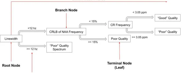
Figure 2.2: An example decision tree for our analysis with the features of a decision tree labeled in bold.

Decision trees are made up of nodes, branches, and leaves (see Figure 2.2). A node is a structure, which contains a condition, if A then B or if not A then C (Quinlan, 1986). All nodes are either terminal, meaning they have no branches or non-terminal, meaning they continue to branch off (Quinlan, 1986). The root node is the first node to any tree and represents the first condition (Quinlan, 1986). Any node with at least a single split is referred to as a branch node (Quinlan, 1986).

The term split means creating two sub-nodes based on a splitting rule on the feature’s characteristics. In Figure 2.2 linewidth has a splitting rule where<12 hz is considered “good” quality or else the spectrum is of “poor” quality. Splitting rules vastly affect the accuracy of the decision tree (see Section 2.6.1.3). Any terminal node is referred to as a leaf (Quinlan, 1986).

These nodes use conditions based on a set of features (Quinlan, 1986; Kuboyama, 2007; James et al., 2017). Features are variables that might be related to class

(43)

membership (Quinlan, 1986; Kuboyama, 2007; James et al., 2017). It should be noted that a feature can appear multiple times in the same tree, however these features do not repeat on the same branch or level (Quinlan, 1986; James et al., 2017). For each terminal node, membership of a particular class is calculated eventually ending in a leaf with the final classification (James et al., 2017). The paths from the root to leaf exhibit the classification rules (James et al., 2017).

We measure a voxel’s spectrum and calculate features of that spectrum, then construct trees to classify “good” or “poor” quality spectra. Due to the classification aspect of the analysis here, decision trees will be referred to classification trees.

A single classification tree is prone to instability as even small changes in the input data can cause radically different results (Louppe et al., 2013; James et al., 2017). Single classification tends to be inaccurate for new observations (Ho, 1995, 1998). However, averaging the classification results in some potentially inaccurate trees all with unique sub-samples of our training set (called “boosting”) can create a more accurate model and is the basis of the random forests approach.

2.6.1.2 Bootstrap Aggregating (Bagging)

As mentioned before, the weakness of a single decision tree is that it lacks stability, which is the degree for which small changes in features affect the overall composition of the tree; slight changes in a subject’s features can drastically change the outcome of the classifier. To defend against this lack of stability, we use ensemble learning with a meta-heuristic approach. Ensemble learning is a strategy in machine learning in which multiple models are fit with a random assortment of features assuming that a good, but not necessarily optimal, model can be created with the expectation that some important variables may have been excluded or missing. A meta-heuristic approach is a higher-level procedure designed to find a sufficiently good solution to an optimization problem with incomplete information (S¨orensen et al., 2018). Sets of solutions are sampled and used in tandem to get results that are not necessarily the globally optimum solution, but rather a sufficiently good one (S¨orensen et al.,

(44)

2018). This kind of modeling approach promotes stability and accuracy while also avoiding overfitting the model (Ho, 1998). Over-fitting being when a model is too closely fit to a limited set of data points causing the model to be only applicable to that very small subset of data points (Ho, 1998). To protect our models from this we use a method called Bootstrap Aggregating or “bagging” (Breiman, 2001).

In bagging, a given training setT withN subjects will createmnew training sets Ti, where i = 1,2, ..., m. Each of these Ti are size N, except that the new training

sets are sampled with replacement. This leads to an expected 1−1/e = 63.2% of Ti being in the bagged sample, with some samples being repeated (Breiman, 2001).

Observations in the bagged training set are referred to as in-bag and observations outside the bagged training set are referred to as out-of-bag observations. These m models are then fitted using the m sub-samples Ti, which are then used to vote

on the proper classifier for individual subjects (Breiman, 2001). This process also improves model performance as it reduces the variance of the model without adding bias (Breiman, 2001).

Now there is an additional bagging done with the features to strengthen our modeling approach, which is aptly referred to as “feature bagging”. This works similarly as described above except that each mmodel also has a unique sub-sample of classification featuresf, this time without replacement. The rule of thumb is with F features to have√F features in each model (Breiman, 2001). This is done to keep the classifier from over-fitting and to allow the user to give many potential features. Ultimately, features with less predictive ability (less “variable importance”) for the classifiers will be removed later with model selection (Breiman, 2001).

2.6.1.3 Splitting Algorithm

Splitting in this case is the point in which an observation is classified in either group based upon its classifications from the individual classification trees. The splitting method for our random forests classifier is Gini index weighted, which determines optimal classification using the formula below from Ishwaran and Kogalur (2007):

(45)

Let ˆp={p1, . . . , pJ} be the class proportions for the classes 1 through J (in this

case 1 to 2 as there are only 2 classes poor and best quality) for the yth outcome of the node.

Suppose the proposed split for the root node is of the formx≤cand x > c for a continuous x-variable x, and a split value of c. The impurity of the node is defined as φ(ˆp) = J X i=j pj(1−pj) = 1− J X j=1 p2_j, j ={1,2}. (2.4)

The Gini index for a split c on x is θ(x, c) = nl

nφ(ˆpl) + nr

nφ(ˆpr), (2.5)

where, as before, the subscripts l and r indicate left and right daughter node mem-bership respectively, and nl and nr are the number of cases in the daughters such

that (n =nl+nr). The goal is to find x and c to minimize the function below.

θ∗(x, c) = nl n 1− J X j=1 nj,l nl 2! +nr nr 1− J X j=1 nj,r ni 2! ,

Where nj,l and nj,r are the number of cases of class j in the left and right daughter,

respectively, such that (nj =nj,l+nj,r). This is equivalent to maximizing the function

below. θ∗(x, c) = 1 n nl− J X j=1 n2_j,l nl ! + 1 n nr− J X j=1 (n2_j,l) nl ! .

Other settings going into the function are the number of trees in the forest, number of features considered for any split, the complexity of each tree, and the sampling scheme. The rule of thumb is to start with Number of features×10 trees (280 in our case), and then trim based on convergence. We found convergence with as few as 100 trees, but we use 1000 for greater error accuracy and because it is quick. By default of the rfsrc function in the “randomForestSRC” package, p/3 features are sampled for each model, which in this case means five variables are being tested in each model. The tree complexity is determined by the size of the nodes in a single tree, which in our case is five.

(46)

2.6.1.4 Out of Bag Error Estimate (OOB)

Methods for testing for classification accuracy are internal or external cross-validation by comparing the model classification with the true labels within the training set or with an additional test or validation set, respectively; random forests incorporates external cross-validation. As mentioned above in Section 2.6.1.2 each tree in the random forests is constructed using a bootstrap sample of the training set. The training sets are constructed with replacement, so about a third of the original cases are excluded. This excluded sub-sample is referred to out-of-bag (OOB) cases.

These excluded cases are then run through the tree to get a classification. At the end of the process these cases are then compared to their actual classification, with j being the class with the most votes every time that case was OOB. The proportion of times j is not equal to the true class of the case is then averaged over all cases, which gives us the OOB error estimate.

This measure of accuracy allows us to rate the quality of the classifications coming out of our model. Through multiple tests it has proven to be unbiased (Breiman, 2001).

2.6.1.5 Variable Importance (VIMP)

Random forests can be used to rank the importance of variables in a regression or classification problem in a natural way. The following technique was described in Breiman’s original paper on the subject and is the one used in the “randomForest-SRC” package by default (Breiman, 2001; Ishwaran and Kogalur, 2007; Ishwaran et al., 2008).

The first step is to fit a random forests classifier to the data. During the fitting process the OOB error estimate for each case is recorded and averaged over the forest. To measure the importance of thekth _{feature after processing, the values of the}

(47)

computed on this new data set. The importance score for thekth _{feature is computed}

by averaging the difference in OOB error over trees with and without the feature. The score is normalized by the standard deviation of these differences, this score is called the VIMP (Breiman, 2001).

Features that score higher are marked as more important than the features that have small values.

There can be an issue in examining variable importance in this manner. For categorical variables with many different levels, random forests are biased to prefer variables with more categories (Breiman, 2001; Ishwaran and Kogalur, 2007). Since our two categorical variables, Cerebellum and Quality map has only a few levels this is not an issue.

Variable importance scores are used to do feature selection on the RFC as well. Using backward selection, the features with the negative VIMP are removed.

2.6.2 Supervised Learning

There are two ways to run a machine learning algorithm, supervised and unsuper-vised; because our training set includes the proper classification for the individual spectra our random forests classifier is supervised.

There are five steps to training our classifier: creating the training set, adding features, determining the structure of the classification model, training the classifier, and assessing the classifier’s accuracy.

Step 1: Create training set. 200 voxels across 20 subjects were selected as a

training set. For each subject 10 voxels were sampled uniformly along the longitu-dinal axis (z-direction) at an interval of roughly one voxel for each 3 z-plane slices. The x and y positions were picked using a random number generator limited by the numbers of brain voxels in both the x and y axis.Each subject had ten sampled voxels with overall, typically seven or six which were of “good” quality, and typically three

(48)

or four of “poor” quality. For an explanation of scoring see Section 2.4.1. Three voxels were then removed after discovering they were located outside of the brain leaving the 197 voxels in the training set. Of these voxels 88 were poor quality and 109 were good quality.

Step 2: Choose features relating to desired outcome. For this analysis a

total of twenty-eight were chosen as potential key variables in measuring the quality of the spectra. See a full write up of each variable in Section 2.3. These features are all output about an individual voxel’s spectra, except for the Cerebellum factor variable which was manually inputted into the data based on voxel location. The goal was to give the classifier as much data on the spectra as possible without pulling the actual spectral image files as those are difficult to create.

Step 3: Determine the structure of the learning function. The learning

structure is described in Section 2.6.1.

Step 4: Run the analysis. The analysis was run with the training set according

to the methods described in Section 2.6.1 with the training set using the features with a “x” in Table 2.1.

Step 5: Output and Diagnostics Both OOB error rates and VIMP scores were

used to determine model accuracy. See Sections 2.6.1.4 and 2.6.1.5 for more details about each of these diagnostic measures.

2.7 Comparison of Filtering Methods

Two sets of data are being compared to measure method effectiveness, the training set of data and the application set of data. Within the training set, we know the true rated quality of the spectra and can compare classification method accuracy.

(49)

For the application set, we can observe the whole-brain patterns of spectral quality and compare those patterns between classification methods.

2.7.1 Examination of Training Set

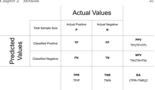
Each method will be used to classify the training set and from this a confusion matrix will be created for each method. The classification statistics of specificity, sensitivity, balance accuracy, positive predictive value, and negative predictive value can be compared across methods. All formulas below are from Fawcett (2006). In the formula outlined below the following acronyms are used:

N - Negative, the number of poor spectra in the training set.

P - Positive, the number of good spectra in the training set.

TN - True Negative, the number of correctly classified poor spectra as determined by the training set.

TP - True Positive, the number of correctly classified good spectra as determined by the training set.

FN - False Negative, the number of incorrectly classified poor spectra.

FP - False Positive, the number of incorrectly classified good spectra.

Sensitivity, or the true positive rate (TPR) is the number of correctly classified good spectra is divided by the number of good spectra in the training set:

TPR = TP

P =

TP

TP + FN (2.6)

The measure tells us about the proportion of each method correctly identifying good quality spectra.

Specificity , or the true negative rate (TNR), is the number of correctly identified poor spectra compared to the number of poor spectra in the training set:

TNR = TN

N =

TN

(50)

Figure 2.3: Details of how to calculate the each statistical measures in Section 2.7.1 using a confusion matrix.

This determines the proportion of our method correctly identifying a poor spectrum. Balanced accuracy (BA) is calculated by averaging the specificity and sensitivity:

BA = T P R+T N R

2 (2.8)

This gives us an overall accuracy of the model taking into account how good the method is at identifying good quality spectra and how good the method is at iden-tifying poor quality spectra.

Positive predictive value (PPV) compares the number of good quality spectra each method classifies and the actual number of good quality spectra in the formula below:

PPV = TP

TP + FP (2.9)

This allows us to compare the number of actual positives to the number of classified positives, giving us an idea about how often our method is over producing positive classifications.

(51)

Negative predictive value (NPV) compares the number of poor quality spectra each method classifies and the actual number of poor quality spectra:

NPV = TN

TN + FN (2.10)

The measure allows us to see how much our model is over or underestimating the number of poor quality spectra

A qualitative comparison will be done on the actual spectra in the training set. The training set voxels will be split into four groups based on the “good” and “poor” ratings of the legacy and RF methods: voxels in which both legacy and random forests methods classified as “good”, voxels in which both legacy and random forests methods classified as “poor”, voxels in which legacy classified as “poor” and random forests methods classified as “good”, and voxels in which legacy methods classified as “good” and RF as “poor”. For each group, five spectra will be randomly selected and plotted on top of each other. This is to see a visualization of what types of voxels are being included and excluded in each method.

2.7.2 Examination of application set

Each of the ten control subjects will have all the voxels of their WB-MSRI brain map of spectra classified as “good” or “poor” by each method, and for each voxel a proportion subjects with a “good” voxel will be calculated to create a map for each method. These maps are called subject inclusion maps with each voxel in the map showing the proportion of subjects with “good” quality spectra or the number of subject’s included in that voxel. The “good” quality maps will then be plotted to compare between models. A table comparing the number of voxels in each method with 100% subject inclusion , 70% subject inclusion, and 50% subject inclusion will also be examined. Images of each map with 100% subject inclusion will also be provided so the differences between the methods can be compared in a spatial sense.

(52)

Chapter 3 Results

In this chapter, we will examine the results of the analyses performed as outlined in Chapter 2. As stated in Section 1.3 we have three aims: Aim 1 is to compare three legacy methods, Maudsley et al. (2006) (MFM), Zhang et al. (2018) (ZFM), and Bustillo et al. (2020) (BFM), to each other; Aim 2 is to train a random forests classifier (RFC) and compare it to the legacy methods; and Aim 3 is to take the vari-ables that scored highest on the RFC and create a random-forests-informed filtering method (RFIFM) that functions similarly to the legacy methods and compare to the legacy methods and the RFC. We will compare the classification statistics for the 5 classification methods using the training set of 197 expert rated spectra. The quali-tative analysis is done by having each method filter ten control subject whole-brain maps. This way we can see the whole-brain patterns of how each method classifies spectra in the brain. To compare methods we will examine the number of voxels that are classified as “good” for each subject, instead of comparing classification accuracy because we do not know the actual good quality spectra in these 10 subjects, and we will examine the actual maps of the combined subjects. These two approaches should give us an idea about how each approach is affecting the final analysis mask.

(53)

3.1 Descriptive data

3.1.1 Training set

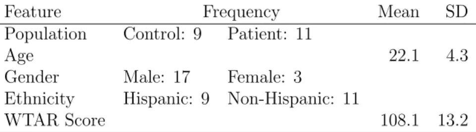
Table 3.1 is a demographics table of the twenty subjects used to sample the 197 voxels. Each subject had ten voxels sampled throughout their brain stratified by z-axis slices.

Table 3.1: Demographics table of training set subjects.

Feature Frequency Mean SD

Population Control: 9 Patient: 11

Age 22.1 4.3

Gender Male: 17 Female: 3

Ethnicity Hispanic: 9 Non-Hispanic: 11

WTAR Score 108.1 13.2

The Wechsler Test of Adult Reading (WTAR) is a commonly used assessment to test intelligence because of its large sampling population. It’s used to both test a subject’s intelligence and to see how that subject’s intelligence score compares to their expected intelligence based on their demographics.

It should be noted that the Bustillo et al. (2020) study for which all subjects are sampled from have a lower proportion of female subjects to male subjects therefore when randomly sampled we sampled fewer female subjects. For the features of interest twenty-eight measures of individual spectra were pulled. The demographics of these spectra can be seen in Table 3.2.

3.1.2 Application set

Ten control subjects were randomly sampled for our application set group. Their spectra were filtered for good quality spectra by all five quality classification methods. Their demographics are in Table 3.3. Note, because our population are entirely control subjects, our WTAR scores are higher than in our training set (Table 3.1). This is expected because patients tend to score lower on their WTAR assessment compared to controls of similar demographics.

An Improved Method for Spectroscopic Quality Classification

UNM Digital Repository

UNM Digital Repository

An Improved Method for Spectroscopic Quality Classification

An Improved Method for Spectroscopic Quality Classification

Elizabeth Grace Mayer

Mathematics & Statistics

Dr. Erik Erdhardt

Dr. Fletcher Christensen

Dr. Rhoshel Lenroot

An Improved Method for Spectroscopic

Quality Classification

Elizabeth Grace Mayer

B.S., UNM, 2017

M.S., UNM, 2020

THESIS

Master of Science

Statistics

Dedication

Acknowledgments

An Improved Method for Spectroscopic

Quality Classification

Elizabeth Grace Mayer

B.S., UNM, 2017

M.S., UNM, 2020

M.S., Statistics, University of New Mexico, 2020

Abstract

Contents

List of Figures

List of Tables

Chapter 1

Introduction

1.1

Magnetic Resonance Spectroscopy (MRS)

stud-ies the concentration of molecules in an object

1.1.1

In-vitro

Magnetic Resonance Spectroscopy

1.1.2

In-vivo

Magnetic Resonance Spectroscopy

1.2

The Importance of Spectral Quality Control

in

in-vivo

MRS

1.2.1

Current practices for Spectral Quality Control in SVS

1.2.2

Current practices for Spectral Quality Control in

WB-MRSI

1.3

Study Aims

Chapter 2

Methods

2.1

Study Design

2.2

Setting and Participants

2.2.1

Training set for Random Forests Classifier and

Classi-fier Statistical Analysis

2.2.2

Application set for Qualitative Assessment

2.3

Features of Spectra and Surrounding Tissue

2.4

Voxel Spectral Quality Classification Ratings

2.4.1

Training Set Spectral Quality

2.5

Data Sources

2.5.1

WB-MRSI Scans

2.6

Statistical Methods

2.6.1

Classification with Machine Learning

2.6.2

Supervised Learning