Singapore Management University
Institutional Knowledge at Singapore Management University
Research Collection School Of Economics
School of Economics
12-2016
Panel data models with interactive fixed effects and
multiple structural breaks
Degui LI
Junhui QIAN
Liangjun SU
Singapore Management University, [email protected]
DOI:https://doi.org/10.1080/01621459.2015.1119696
Follow this and additional works at:
https://ink.library.smu.edu.sg/soe_research
Part of the
Econometrics Commons
This Journal Article is brought to you for free and open access by the School of Economics at Institutional Knowledge at Singapore Management University. It has been accepted for inclusion in Research Collection School Of Economics by an authorized administrator of Institutional Knowledge at Singapore Management University. For more information, please [email protected].
Citation
LI, Degui; QIAN, Junhui; and SU, Liangjun. Panel data models with interactive fixed effects and multiple structural breaks. (2016).
Journal of the American Statistical Association. 111, (516), 1804-1819. Research Collection School Of Economics.
Panel Data Models with Interactive Fixed E
ff
ects and Multiple
Structural Breaks
∗
Degui Li
†,
Junhui Qian
‡, Liangjun Su
§University of York, Shanghai Jiao Tong University, Singapore Management University
September 12, 2015
Abstract
In this paper we consider estimation of common structural breaks in panel data models with unobservable interactivefixed effects. We introduce a penalized principal component (PPC) estimation procedure with an adaptive group fused LASSO to detect the multiple structural breaks in the models. Under some mild conditions, we show that with probabil-ity approaching one the proposed method can correctly determine the unknown number of breaks and consistently estimate the common break dates. Furthermore, we estimate the regression coefficients through the post-LASSO method and establish the asymptotic dis-tribution theory for the resulting estimators. The developed methodology and theory are applicable to the case of dynamic panel data models. Simulation results demonstrate that the proposed method works well infinite samples with low false detection probability when there is no structural break and high probability of correctly estimating the break numbers when the structural breaks exist. Wefinally apply our method to study the environmental Kuznets curve for 74 countries over 40 years and detect two breaks in the data.
Keywords: Change point; Interactivefixed effects; LASSO; Panel data; Penalized estimation; Principal component analysis.
∗The authors sincerely thank the editor, an associate editor, and two referees for the helpful and insightful
comments which have led to a substantial improvement of the paper. Su gratefully acknowledges the Singapore Ministry of Education for Academic Research Fund under grant number MOE2012-T2-2-021.
†Department of Mathematics, University of York, Heslington, York, YO10 5DD, United Kingdom. Email: [email protected].
‡Antai College of Economics and Management, Shanghai Jiao Tong University, Shanghai 200052, China. Email: [email protected].
§School of Economics, Singapore Management University, Singapore 178903, Singapore. Email: [email protected].
Published in Journal of the American Statistical Association, October 2016, Volume 111, Issue 516, pp. 1804-1819. Pre-print version.
1
Introduction
As the availability of panel or longitudinal data increases in the last few decades, panel data studies have become increasingly popular among a wide group of statisticians and econome-tricians. Analysis of panel data sets has various advantages over that of purely time series or cross-sectional data sets. A relatively less exploited advantage of the panel data is that it pro-vides researchers with moreflexibility to model cross-sectional dependence over individual units and uncover possible structural changes over time. Structural breaks are, indeed, quite common in many areas such as economics and finance, and may occur for various reasons. For example, the celebrated environmental Kuznets curve may shift as a result of a growing public awareness of environmental issues, a technological breakthrough, or an international coordination and co-operation on environmental protection. If such structural changes are ignored in the modelling, subsequent statistical analyses may lead to incorrect inferences or misleading predictions.
In recent years, there has been a growing literature on the estimation and test of structural breaks in panel data models. Generally speaking, most of the existing literature falls into two categories depending on whether the parameters of interest are allowed to be heterogenous across subjects or not. Thefirst category focuses on homogenous panel data models (e.g., De Watcher and Tzavalis, 2012; and Qian and Su, 2015b) and the second category considers estimation and inference of common breaks in heterogenous panel data models (e.g., Bai, 2010; Kim, 2011; Baltagi et al., 2015). Despite the vast literature on multiple structural breaks in the time series framework (e.g., Csörgö and Horváth, 1997; Bai and Perron, 1998; Qu and Perron, 2007; Harchaoui and Lèvy-Leduc, 2010; Chan et al., 2014; Qian and Su, 2015a), most of the existing work on panel structural breaks focuses on the estimation and inference of a single structural break in panel data models. The only exception is the paper by Qian and Su (2015b) which considers shrinkage estimation of common breaks in panel data models. However, Qian and Su’s (2015b) modelling framework does not allow the existence of cross-sectional dependence, which limits the applicability of their techniques as cross-sectional dependence commonly exists in many panel data sets nowadays (such as the panel climate and environmental data).
In this paper, we aim to estimate multiple structural breaks in panel data models with cross-sectional dependence which is described through the unobservable interactivefixed effects. Such a cross-sectional dependence structure has received increasing interest in the analysis of panel data in recent years; see Pesaran (2006), Bai (2009), Bai and Li (2014), and Moon and Weidner (2014, 2015), among others. However, to the best of our knowledge, there is virtually no
work on estimating multiple structural breaks in panel data models with interactivefixed effects and possible dynamic structure (such as the dynamic autoregressive panel data models). As in Qian and Su (2015b), we apply the shrinkage idea through the adaptive group fused LASSO (AGF-LASSO) to estimate the multiple structural break dates. Nevertheless, the existence of the unobservable interactive fixed effects in our model makes the estimation techniques and the development of the asymptotic theory much more involved than those in Qian and Su (2015b). In Section 2 below, we introduce a novel penalized principal component (PPC) estimation procedure via AGF-LASSO to estimate both the regression coefficients and the factor loadings. Similar to the sparsity result in the high-dimensional variable selection literature (e.g., Fan and Li, 2001, 2006), we establish the consistency for the detection of multiple structural breaks, which indicates that both the number of breaks and the break dates can be consistently estimated. Furthermore, we also estimate the regression coefficients through the post-LASSO method and then establish the asymptotic distribution theory of the resulting estimators, which generalizes the results in Bai (2009) and Moon and Weidner (2014) where there is no structural break. The simulation studies show that the proposed PPC method has a high probability of correctly estimating the number of breaks when the structural breaks exist in panel data models, and a low probability of false detection when there is no structural break. Furthermore, we study the environmental Kuznets curve for 74 countries over 40 years by using our method andfind that there exist two structural breaks in the data.
The rest of the paper is organized as follows. Section 2 introduces the model and the PPC estimation method. Section 3 gives the asymptotic properties for the PPC estimator as well as the post-LASSO estimator. Section 4 discusses the determination of the number of the factors and the choice of the tuning parameter in the PPC estimation procedure and reports the Monte Carlo simulation results. Section 5 gives the empirical application of the proposed model and method. Section 6 concludes the paper. Appendices A and B give the assumptions and the proofs of the asymptotic results, respectively. Some technical lemmas as well as their proofs are collected in Appendix C of the supplemental document.
Notation. For an × real matrixA we denote its transpose asA0its Frobenius norm as kAk (≡ [tr(AA0)]12) its spectral norm as kAk
sp(≡ [max(AA0)] 12
) and its Moore-Penrose generalized inverse asA+where max(·) denotes the maximum eigenvalue of a square matrix. Let P =A(A0A)+A0 and M =I−P where I is an × identity matrix. When A is symmetric with = , we use (A) to denote its th largest eigenvalue by counting multiple eigenvalues multiple times, andmax(A)andmin(A)to denote the largest and smallest
eigenvalues of A, respectively. Let vec(A) be the vectorization of A and Tr(A) the trace of a square matrixA. Let0 denote a null matrix or vector whose size may change from line to line, and 1{·} be the usual indicator function. The operator → denotes convergence in probability,
→ convergence in distribution, and plim probability limit. We use ( ) → ∞to denote that both and pass to infinity jointly.
2
Model and estimation
In this section, we first introduce a panel data model with interactive fixed effects and an unknown number of structural breaks, and then propose the PPC estimation method.
2.1
The model
Let be the dependent variable for subject measured at time where = 1 and
= 1 . We consider the following panel data model with interactivefixed effects
=0+0+ = 1 = 1 (2.1) where is a ×1 vector of explanatory variables, is a ×1 vector of unknown slope coefficients which may change over time,anddenote an0×1vector of unobservable factor
loadings and common factors, respectively, both of which may be correlated with , and is the idiosyncratic error term. The dimension of the unknown coefficient vector, ≡ , is allowed to be diverging as( )→ ∞, and the dimension of the vectors for the factor loadings and common factors,0, is afixed positive integer. Throughout the paper, we denote the true
value of a parameter vector with a superscript 0. For instance, 0, 0 and 0
denote the true values of , and , respectively. We allow the regression coefficients to vary over the time and model (2.1) thus includes the classical linear panel data models with interactivefixed effects (e.g., Pesaran, 2006; Bai, 2009; Moon and Weidner, 2015) as a special case. As in these papers, we assume that both the cross-sectional size and the time series length pass to infinity, which is called as “large dimensional panel” in the literature.
In this paper we assume that the true regression coefficients ©01 0ª exhibit certain
sparse nature such that the total number of distinct vectors in the set is given by0+ 1which
is unknown but typically much smaller than the time series length. We allow0 ≡0 to be divergent at an appropriate rate as → ∞. More specifically, we let
where we adopt the convention that 00 = 1 and 00+1 = + 1The indices 0, = 1 0, indicate that there are 0 unobserved break points/dates and the number 0+ 1 denotes the total number of regimes. We are interested in estimating the unknown number of structural breaks, the unobservable break dates, and the regression coefficients in different regimes. Let β = ¡01 0¢0 α = (01 0+1)0Λ = ¡ 1 2 ¢0 F = ¡ 1 2 ¢0 and T =
(1 )Throughout the paper, we use0α00 =
¡ 00 1 000+1 ¢0and T0 0 = ¡ 0 1 00 ¢
to denote the true number of structural breaks, the true vector of distinct regression coefficients, and the set of true break dates, respectively.
2.2
PPC estimation
We consider the PPC estimation of the unknown components ¡β0Λ0F0¢, the true values of
¡ βΛF¢. Let= ¡ 1 ¢0 and = ¡ 1
¢0. In order to apply the PPC method, we define the objective function through
˜ ¡βΛF¢= 1 X =1 X =1 ¡ −0 −0¢2+ X =2 ˙ ° °−−1°° (2.2)
which can be written as
1 X =1 (−−Λ)0(−−Λ) + X =2 ˙ ° °−−1°° where≡ 0 is a tuning parameter and˙ is a data-driven weight defined by
˙ = ° °˙ −˙−1 ° °− = 2 (2.3) ˙
, = 1 , are the preliminary estimates of the regression coefficients, and is a user-specified positive constant that usually takes value 2 in the literature. In this paper, the pre-liminary estimation ©˙ = 1 ª is constructed to minimize thefirst term of the objective function in (2.2) by ignoring the penalization device.
By concentratingF out in thefirst term of the objective function (2.2), we can readily obtain the following objective function
ˆ (βΛ) = ˆ (βΛ) + X =2 ˙ ° °−−1°° (2.4)
whereˆ (βΛ) = 1 P=1(−)0MΛ(−)Following Moon and Weidner (2014), we can further concentrate Λ out in (2.4) and obtain the objective function
¯ (β) = ¯ (β) + X =2 ˙ ° °−−1°° (2.5)
where ¯ (β) = 1 X =0+1 " 1 X =1 (−) (−)0 # (2.6)
It can be seen that the penalization device in the above objective functions is closely related to the literature on the adaptive LASSO (Zou, 2006), the group LASSO (Yuan and Lin, 2006), and the fused LASSO (Tibshirani et al., 2005; Rinaldo, 2009). The use of the Frobenius normk·k for the vector difference−−1 generalizes the fused LASSO to the group fused LASSO; and the use of the weights {˙} makes the LASSO procedure adaptive. Therefore, we can call our penalized estimation procedure as anadaptive group fused LASSO (AGF-LASSO) procedure.
Following Bai and Ng’s (2002) principal component method under the identification restric-tions thatΛ0Λ =I0 andF0F is a diagonal matrix, the minimizers to the objective function defined in (2.4), βˆ =¡ˆ01 ˆ0¢0 and Λˆ satisfy that
ˆ β= arg min ˆ (βΛ)ˆ (2.7) and h 1 X =1 ¡ −ˆ ¢¡ −ˆ ¢0iˆ Λ= ˆΛV (2.8)
where V is a diagonal matrix consisting of the 0 largest eigenvalues of the matrix in the
square brackets in (2.8) arranged in descending order. Furthermore, the common factorF0 can be estimated by
ˆ
F = ( ˆ1ˆ2 ˆ)0 with ˆ=−1Λˆ0(−ˆ) (2.9) An iterative algorithm based on (2.7) and (2.8) can be implemented in practice to estimate β0 andΛ0. Note that the above calculations are different from those in the existing literature such as Bai (2009) and Lu and Su (2015) by switching the role of Λ and F, because the regression coefficients are heterogeneous over time.
With the estimated regression coefficients ˆ, the set of estimated break dates are given by Tˆˆ = ( ˆ1 ˆˆ) where 2 ≤ ˆ1 ˆˆ ≤ such that kˆ −ˆ−1k 6= 0 at = ˆ for = 1 ˆ. The set Tˆˆ divides the time interval [1 ] into ˆ + 1 regimes such that the
parameter estimates remain constant within each regime. Notice that ifˆˆ =the last break
occurs at the end of the sample and the( ˆ+ 1)th regime has only one time series observation for each cross-sectional unit. Let ˆ0 = 1and ˆˆ+1=+ 1. Define ˆ = ˆ( ˆTˆ) = ˆˆ
−1 as the estimate of 0 for = 1 ˆ + 1In the sequel, we usually suppress the dependence of ˆ on
ˆ
Tˆ (or the tuning parameter ) unless necessary. For example, we letαˆˆ =
¡ ˆ 01ˆ02 ˆ0ˆ+1¢0 which denotesαˆˆ( ˆTˆ) = £ ˆ 1( ˆTˆ)0ˆ2( ˆTˆ)0 ˆˆ+1( ˆTˆ)0 ¤0
3
Asymptotic properties
In this section, we give the large sample theory including the consistency of the proposed PPC estimator and the limiting distribution of the post-LASSO estimator.
3.1
Consistency of the PPC estimator
We start with the consistency result of the PPC estimatorβˆ with preliminary convergence rates.
Theorem 3.1 Suppose that Assumptions 1 and 2(i)-(ii) in Appendix A holds. Then we have (i) °°βˆ −β0°°2 = (+ 1) = ³ − 2 ´, and (ii) ° ° °ˆ−0 ° ° ° = ³ − 1 ´, where = min( p √).
Theorems 3.1 (i) and (ii) establish the preliminary mean square and point-wise convergence rates of {ˆ} respectively, which is a very general result by allowing the existence of multiple jumps or drops in the regression coefficients. As we allow the regression coefficients to vary over time, there is less observational information available for the estimation of each regression coefficient (compared with the model without any structural break). This would in turn affect the estimation accuracy of the factor loading matrix and convergence rates for the parameter estimators. The divergent dimension of the regression coefficients at each time point further slows down the convergence rates. Note that the total number of the unknown elements in the set{0}is. Hence, it is not surprising that in Theorem 3.1 we can only obtain the
¡
− 1 ¢ convergence rate for the PPC estimator ˆ, which is much slower than the optimal root-( )
rate obtained by Bai (2009) and Moon and Weidner (2014) (after bias correction) when there is no change point for the regression coefficients and the dimension of the regression coefficients is
fixed.
Recall that T00 =
©
10 00
ª
denotes the set of true break dates. Let T = {2 } \T00. Let 01 =01,ˆ1 = ˆ1, 0 =0 −0−1 and ˆ = ˆ−ˆ−1 for = 2 The following
theorem establishes the detection consistency, which, in some sense, is analogous to the sparsity result in the high-dimensional variable selection literature.
Theorem 3.2 Suppose that Assumptions 1 and 2 in Appendix A hold. Thenlim()→∞P¡°°ˆ
° °= 0 for all ∈T¢= 1
Theorem 3.2 shows that with probability approaching one (w.p.a.1), all the zero vectors in ©0ª must be estimated as exactly zero, which is a well-known sparsity result in the high-dimensional variable selection literature (c.f., Fan and Li, 2006). On the other hand, by Theorem
3.1(ii), we know that the estimators of the nonzero vectors in©0ªare consistent by noting that
ˆ
−ˆ−1 consistently estimates0=0−0−1. A combination of Theorems 3.1 and 3.2 implies that the AGF-LASSO penalty has the ability to identify the true regression model with the correct number of structural breaks and the correct break dates, which is stated in the following corollary.
Corollary 3.3 Suppose that Assumptions 1 and 2 in Appendix A hold. Then (i)lim()→∞P( ˆ =0) = 1 and (ii) lim()→∞P( ˆ1=10 ˆ0 =0
0) = 1
3.2
Post-LASSO estimation
We next introduce the post-LASSO estimation of the regression coefficients, which can improve the convergence rate of the PPC estimation given in Theorem 3.1. For any(+ 1)-dimensional vector α = ¡ 0 1 0+1 ¢0 and T ={1 } with 1 1 ≤we define the objective function by ¡αΛF;T¢ = 1 X+1 =1 −1 X =−1 X =1 ¡ −0 −0¢2 = 1 X+1 =1 X−1 =−1 (−−Λ)0(−−Λ) (3.1)
By concentrating F out in the above objective function, we readily obtain the following post-LASSO objective function
¡ αΛ;T ¢ = 1 X+1 =1 X−1 =−1 ¡ − ¢0 MΛ ¡ − ¢ (3.2) Let α˜ (T) = £ ˜ 1(T)0 ˜+1(T)0 ¤0 and Λ˜(T) = £˜ 1(T) ˜(T) ¤0
denote the mini-mizers of the objective function defined in (3.2) for givenTBy settingTasTˆˆ = ( ˆ1 ˆˆ),
the set of the estimated break dates constructed in Section 2.2, we obtain the post-LASSO es-timators α˜ˆ ≡α˜ˆ( ˆTˆ)and Λ˜ ≡Λ( ˆ˜ Tˆ).
We next study the asymptotic distribution of the post-LASSO estimators. Corollary 3.3 above implies that w.p.a.1 ˆ = 0 and ˆ = 0 for = 1 0. Hence, it follows that ˜ˆ
is asymptotically equivalent to the infeasible estimator α˜0(T0) which is obtained only if one knows the set T0
0 of the true break dates. Let() =0−0−1,
B (1) = £ 1(1)0 0+1(1)0 ¤0 and B (2) = £ 1(21)0− 1(22)0 0+1(21)0− 0+1(22)0 ¤0
where for = 1 0+ 1 (1) = 1 2 () 0 −1 X =0 −1 0MΛ˜ 0εε 0Λ˜ 0 ¡1 Λ 00Λ˜ 0 ¢+¡1 F 00F0¢+0 (21) = 1 () 0 −1 X =0 −1 0Λ0¡1 Λ 00Λ0¢+¡1 F 00F0¢+¡ 1 X =1 00 ¢ (22) = 1 () 0 −1 X =0 −1 0Λ0¡1 Λ 00Λ0¢+¡1 F 00F0¢+¡ 1 X =1 00∗¢ and ∗ = 1 P=1 with = 00 ¡1 F 00F0¢+0 , ε = (1 ) with = ¡ 1 ¢0. We then define B =Ω+ £ B (1) +B (2)−B (3) ¤ whereΩ andB (3)are defined in Appendix A. Let
D =diag np 1() q 0+1() o ⊗I
where ⊗denotes the Kronecker product, andS be a0×(0+ 1)matrix with full row rank
and 0 being a fixed positive integer.
Theorem 3.4 Suppose that Assumptions 1—3 in Appendix A hold. Then conditional on ˆ = 0we have SD ¡ ˜ αˆ −α0+B ¢ −→N¡0 SΩ+0Ω1Ω+0S0 ¢
where Ω0 andΩ1 are defined in Assumption 3 in Appendix A.
Despite the use of different notations and proof strategies, Ω+ B (1) and Ω+ B (2) correspond to the terms − and − in Bai (2009) or −−13 and −−12 in Moon and
Weidner (2014), respectively. However, these two papers assume that the dimension is fixed and there is no structural break on the regression coefficients. Hence, our asymptotic distribution theory is derived under a more general framework. Like the term−−11in Moon and Weidner
(2014), Ω+ B (3) arises here because we allow the regressor vector to contain lagged dependent variable (e.g., −1) and it is vanishing under Bai’s (2009) conditions A-E that
include the independence betweenand( 0 0)for all and thus rule out dynamics in the regression equation. As Bai (2009) remarks, in the absence of both serial/cross-sectional correlations and heteroskedasticity and under his Assumption D, all of these three bias terms are
asymptotically negligible. In the general case, the bias terms of the post-LASSO estimates can be removed by constructing a bias-corrected estimate. Following Bai (2009) in the case of static panels or Moon and Weidner (2014) in the case of dynamic panels, one can easily construct a bias corrected version of our post-LASSO estimate. We omit the details as the extension is quite straightforward.
Note that the above theorem holds without requiring that and diverge to infinity at the same speed and the latter condition was assumed in both Bai (2009) and Moon and Weidner (2014). For the easiness of presentation, we need to assume that () =0−0−1 ∝ 0 in
Assumption 3(ii) in Appendix A, which implies that each regime-specific regression coefficient vector0 can be estimated at the same convergence rate (
p
0( ))after possible bias
correction. Apparently, it is possible to weaken this last assumption to0−0−1 → ∞and then we anticipate that ˜(T)’s would have different convergence rates to their true values across different regimes.
4
Practical issues in model estimation and simulation study
In this section we first discuss the determination of the number of factors and the choice of the tuning parameterin the PPC estimation procedure, then introduce the algorithm to implement the estimation method, and finally conduct a set of Monte Carlo experiments to evaluate the
finite sample performance of the proposed method.
4.1
Determination of the number of factors
In the above analysis we assume that the number of factors0 is known. In practice, one has to
determine it from data. Here we useto denote a generic number of factors and assume that it is bounded from above by a finite integer max ≥ 0 We propose a BIC-type information
criterion to determine0 before embarking on the AGF-LASSO procedure.
Let ˙˙ and ˙ denote the PCA estimators (without the penalization device) of
andby assuming factors in the model using the normalization rule: Λ0Λ =I and F0F is a diagonal. Note that we have made the dependence of the parameters and their estimators onexplicitly here. Letβ˙=
³ ˙ 01 ˙0 ´0 Define (β˙) = 1 X =+1 " 1 X =1 ³ −˙ ´ ³ −˙ ´0#
Following Bai and Ng (2002), we consider the BIC-type information criterion defined by
BIC() = ln(β˙) +1 (4.1)
where 1 ≡ 1 is pre-determined which plays the role of ln ( )( ) in the case of the conventional BIC criterion. Let ˆ = arg min0≤≤maxBIC(), which estimates the number of the factors.
Theorem 4.1 Suppose that Assumptions 1—4 in Appendix A hold. Then
P³ˆ =0
´
→1 as ( )→ ∞.
The above theorem shows that the use ofBIC()can consistently estimate0To implement
the above information criterion, one needs to choose the penalty coefficient 1. Following Bai and Ng (2002), we can set
1 = ( +) ln µ + ¶ or 1 = ( +) ln ¡ 2 ¢ where = min{ √
√} is defined as in Section 3. The penalty coefficient in Bai and Ng (2002) corresponds to = 1 in the above definitions of 1In our simulations we use the first specification of 1 and search forˆ in the range of {12 5} when 0 = 2.
4.2
Choice of the tuning parameter
We now discuss the choice of the tuning parameter in the PPC estimation procedure, which is an important issue when the penalized methodology is used in practice. Let
˜ αˆ = ˜αˆ( ˆTˆ) = £ ˜ 1( ˆTˆ) 0 ˜ ˆ +1( ˆTˆ) 0¤0
denote the set of the post-LASSO estimates of the regression coefficients based on the break dates in Tˆˆ = ˆTˆ(), where we make the dependence of various estimates on explicitly. Let ˜2( ˆTˆ) =
¡
˜
αˆΛ˜F˜; ˆTˆ
¢
, where F˜ is defined similarly to Fˆ in (2.9) with Λˆ and
ˆ
replaced by Λ˜ and ˜( ˆTˆ) when ˆ−1 ≤ ≤ˆ −1. We then propose to select the tuning parameter by minimizing the following information criterion:
IC() = ln£˜2( ˆTˆ)
¤
+2¡ˆ+ 1
¢
(4.2)
Theorem 4.2 Suppose that Assumptions 1—2 and 3(ii) and 5 in Appendix A hold. Then
P¡ˆˆ=0
¢
→1 as ( )→ ∞
The above theorem shows that by minimizing IC(), we can obtain a data-driven ˆ that ensures the correct determination of the number of breaks. When we minimize the objective function in (4.2), we do not restrict to satisfy Assumptions 3(i) and (iii) in Appendix A. If these two additional conditions also hold, we know from Corollary 3.3 that ˆˆ =0 w.p.a.1. But in practice, it is hard to ensure such conditions and Theorem 4.2 becomes handy.
In the following simulation, we choose2 =log(min( ))min( ), whereis a positive constant. This choice of 2 satisfies the two restrictions specified above. To implement the information criterion in practice, we find an upper bound for the tuning parameter,max, that would yield zero break in every data generating process (DGP), and a lower bound min that would yield many breaks. We then search for the optimal tuning parameter on the 20 evenly-distributed logarithmic grids in the interval [min max]. To determine , we use a data-driven method that is similar to the one in Hallin and Liska (2007). Specifically, given an 0 0, we examine subsamples ( ), = 1 , = 1 , where = 1 and
0 1 · · · =. Note that we do not consider subsamples along the time dimension because we allow for structural breaks over time. We examine a range of possible values for , say [min max], where min leads to a large number of breaks and max leads to zero break
for all choices of . For each , we find the number of breaks in each subsample, ˆ, with
= 1 . Let ¯ = 1 P=1ˆ, we select the smallest ∈ [min max] that satisfies =
1
P
=1( ˆ−¯)2 = 0 and ¯ −1. Intuitively, the constant should be chosen such that the estimated number of breaks is constant across the subsamples, given the intuitive explanation in Hallin and Liska (2007). In our simulations we set =−+and = 3to save computation time.
4.3
Implementation of the estimation method
The implementation of the PPC estimation method consists of two steps. In thefirst step, the preliminary estimation ˙ is obtained along with the estimated number of factors ˆ. Given a generic number of factors, ˙ is obtained by minimizing the first term of ˜
¡
βΛF¢ in (2.2). The minimization problem is solved using an iterative algorithm based on (2.7) and (2.8) with ˆ (βΛ)ˆ replaced by ˆ (βΛ)ˆ , the first term of ˆ (βΛ)ˆ . The starting values
for the iteration are chosen to be the pooled least squares estimates, assuming that coefficients are time-invariant and that no factor structure exists.
In the second step, given a generic tuning parameter , we use the following iterative al-gorithm to minimize ˆ
¡
βΛ¢ in (2.4), yielding the set of breaks corresponding to . Let 1 =1 and =−−1,= 2 , and let θ= (1 )0.
(1) Initializeθ(0), which implies an initial set of breaks and parameter estimates in each regime. (2) Givenθ(−1) (and thusβ()), calculate factor loadingsΛ()using eigenvalue decomposition,
where the superscript () denotes the -th iteration.
(3) GivenΛ(), updateθ() (or equivalently β()) that minimizesˆ (βΛ())in (2.4). This calculation utilizes a block-coordinate-descent algorithm similar to that used in Qian and Su (2015b). The updatedθ() implies a new set of breaks, and the post-LASSO procedure is used to obtain new estimates of parameters in each regime.
(4) Repeat (2)-(3) untilkθ()−θ(−1)kdrops below a pre-determined threshold. Use the post-LASSO procedure to obtain the final estimate of parameters, factors and their loadings. In the above iterative algorithm, the starting values for the iterations are chosen to be the preliminary estimates of the coefficients obtained in thefirst step. The post-LASSO procedure minimizes
¡
αΛF;T
¢
in (3.1) with T replaced by the estimated set of break dates in each iteration and with the starting values chosen to be the pooled least squares estimates as in the first step. Finally, we obtain the set of break dates using the tuning parameter that minimizesIC() defined in (4.2).
4.4
Simulation
We consider the following data generating processes:
=1+2+0+ = 1 = 1 where= £ (1) (2) ¤0 and= £ (1) (2) ¤0
are two-dimensional random vectors, and • DGP-1 (benchmark): ∼ N(01),= 1, ∼ N(0I2), ∼ N(0I2), both and are independent of,
• DGP-2 (serial correlation in the common factor and heteroskedasticity in the error): ,
, and are defined as in DGP-1, each of the two element in is an AR(1) process with unit variance: () = 05−1() +() with =
£ (1) (2) ¤0 ∼ N(0075I2), = ¡ 075 + 0152 ¢12 ∗ with ∗
∼ N(01)and independent of, and ; • DGP-3 (dependent factors and serial correlation in the error): = 050+ 05(0+
0) +¦ with ¦ ∼ N(01) and = (11)0, and are defined as in DGP-1, is defined as in DGP-2, for each , is an independent ARMA(1,1) process with unit variance such that= 05−1+ + 05−1, where
∼ N(037); • DGP-4 (dynamic panel): =−1,
∼ N(01),andare defined as in DGP-1,
is defined as in DGP-2.
In order to evaluate the performance under different noise levels, we select the free parameter to be either 0.5 or 1. In DGP-1 with no breaks,= 1roughly corresponds to a signal-to-noise ratio of 1. We also experiment on different levels of factor loadings and find that the impact of the magnitude of the factor loadings on the performance of our method is small.
DGP-1 serves as the benchmark case where both the regressor and the idiosyncratic error are sequences of strong white noise. DGP-2 introduces serial correlation in the common factor and conditional heteroskedasticity in the model errors. DGP-3 allows the dependence of both the factor loadings and common factors on the regressor. In addition, DGP-3 introduces serial correlation into the model errors. DGP-4 has a dynamic panel AR(1) structure. We experiment on four combinations of dimensions: ( ) = (4040), ( ) = (8040), ( ) = (4080), and ( ) = (8080). The data-driven method to select both the constant in 2 and the tuning parameteris computationally intensive. As a result, we set the number of Monte Carlo replications to be 250.
For the DGPs 1—3, we set 1 =2 = 1 for all when no break exists, 1 =2=1{1 ≤ ≤ 2} when there is one break, and 1=2=1{1≤≤b 3c}+1{ 2 ≤} when there are two breaks. For the DGP-4, we set 1 =2 = 05 for all when there is no break, 1 =2 = 05·1{1≤≤ 2} when there is only one break, and1=2 = 05·1{1≤≤ b 3c}+ 05·1{ 2 ≤} when there are two breaks.
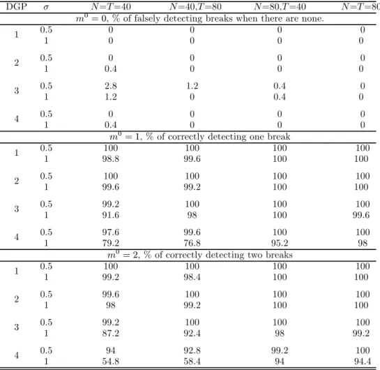
We first evaluate the probability of falsely detecting breaks when there is no break in the simulation design. Then we experiment on the DGPs with one or two breaks. We evaluate the probability of correctly detecting the number of breaks and the accuracy of break date estimation when breaks are detected. Tables 1, 2, and 3 report simulation results for the above DGPs. The
Table 1: The probabilities for falsely detecting breaks when there are none and of correctly detecting the breaks when there are breaks
DGP ==40 =40,=80 =80,=40 ==80
0= 0, % of falsely detecting breaks when there are none.
0.5 0 0 0 0 1 1 0 0 0 0 0.5 0 0 0 0 2 1 0.4 0 0 0 0.5 2.8 1.2 0.4 0 3 1 1.2 0 0.4 0 0.5 0 0 0 0 4 1 0.4 0 0 0
0= 1, % of correctly detecting one break
0.5 100 100 100 100 1 1 98.8 99.6 100 100 0.5 100 100 100 100 2 1 99.6 99.2 100 100 0.5 99.2 100 100 100 3 1 91.6 98 100 99.6 0.5 97.6 99.6 100 100 4 1 79.2 76.8 95.2 98
0= 2, % of correctly detecting two breaks
0.5 100 100 100 100 1 1 99.2 98.4 100 100 0.5 99.6 100 100 100 2 1 98 99.2 100 100 0.5 99.2 100 100 100 3 1 87.2 92.4 98 99.2 0.5 94 92.8 99.2 100 4 1 54.8 58.4 94 94.4
first panel of Table 1 reports the percentages of falsely detecting breaks when there is no break (0 = 0). The second and the third panels report the percentages of correctly estimating the number of breaks when the true number of breaks is one and two, respectively. In Table 2, we report the ratio of average Hausdorff distance (HD) between the estimated and true sets of breaks to , i.e., 100·HD(TbT0
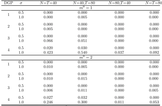
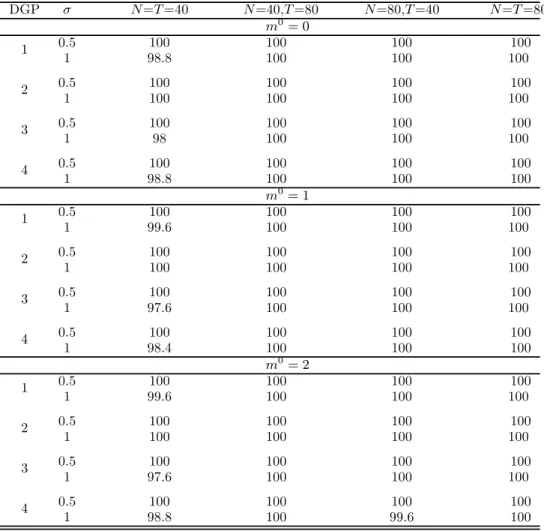
0), conditional on correct estimation of the number of breaks. Here the average is taken over 250 replications and the HD between two sets and is defined as HD( ) = max{D( ) D( )} with D( ) ≡ sup∈inf∈|−|. The mean squared or absolute errors of the parameter estimates are roughly proportional to the Hausdorfferror of the break-date estimation and hence are not reported. In Table 3 we report the percentages of correctly estimating the number of factors in the Monte Carlo replications.
Table 2: Estimation accuracy for the break dates when there is one or two structural breaks DGP ==40 =40,=80 =80,=40 ==80 0 = 1 0.5 0.000 0.000 0.000 0.000 1 1.0 0.000 0.005 0.000 0.000 0.5 0.000 0.000 0.000 0.000 2 1.0 0.005 0.000 0.000 0.000 0.5 0.000 0.000 0.000 0.000 3 1.0 0.066 0.051 0.000 0.000 0.5 0.020 0.030 0.000 0.000 4 1.0 0.423 0.540 0.037 0.092 0 = 2 0.5 0.000 0.000 0.000 0.000 1 1.0 0.010 0.005 0.000 0.000 0.5 0.000 0.000 0.000 0.000 2 1.0 0.010 0.015 0.000 0.000 0.5 0.000 0.000 0.000 0.000 3 1.0 0.006 0.011 0.000 0.005 0.5 0.027 0.032 0.000 0.000 4 1.0 0.246 0.300 0.011 0.053
Note. The table reports100·HD(TT00)averaged over 250 replications.
We summarize the major findings from these tables. (i) When there is no break in the DGPs, the probabilities of falsely detecting breaks decline to zero as either or increases. (ii) When there are one or two breaks, the probabilities of correctly estimating the number of breaks increase fairly quickly to 100% or near 100% as both and increase. The detection procedure performs slightly better at lower idiosyncratic noise levels ( = 05) than at higher noise level ( = 1). The performance is robust to serial correlation in the common factor, serial correlation and conditional heteroskedasticity in the errors, and the dependence of both the factors and their loadings on the regressor. For the dynamic panel (DGP-4), the procedure performs less satisfactorily. However, this may be due to the fact that the signal-to-noise ratio in this case is roughly13, much less than that in the other three DGPs. (iii) Conditional on the correct estimation of the number of breaks, our procedure estimates the break dates accurately, which can be seen from Table 2. (iv) Finally, Table 3 shows that the BIC-type information criterion specified in (4.1) can accurately determine the number of factors for the interactive
Table 3: The probabilities for correctly estimating the number of factors DGP ==40 =40,=80 =80,=40 ==80 0= 0 0.5 100 100 100 100 1 1 98.8 100 100 100 0.5 100 100 100 100 2 1 100 100 100 100 0.5 100 100 100 100 3 1 98 100 100 100 0.5 100 100 100 100 4 1 98.8 100 100 100 0= 1 0.5 100 100 100 100 1 1 99.6 100 100 100 0.5 100 100 100 100 2 1 100 100 100 100 0.5 100 100 100 100 3 1 97.6 100 100 100 0.5 100 100 100 100 4 1 98.4 100 100 100 0= 2 0.5 100 100 100 100 1 1 99.6 100 100 100 0.5 100 100 100 100 2 1 100 100 100 100 0.5 100 100 100 100 3 1 97.6 100 100 100 0.5 100 100 100 100 4 1 98.8 100 99.6 100
5
An empirical application to the environmental Kuznets curve
The environmental Kuznets curve (EKC) has become a standard feature in the environmental policy literature. It hypothesizes that the relationship between income and the emission of chemicals like sulfur dioxide (SO2) and carbon dioxide (CO2) or the natural resource usage hasan inverted U-shape, which is similar to the relationship between income and inequality in the Kuznets curve hypothesis in economics. In this section we consider the following specification:
=0+1+22+3+0+
whererepresents the logarithm of per capita CO2emission for countryin year,represents the logarithm of per capita income in 2000 USD (gross domestic product, abbreviated as GDP), represents the logarithm of per capita consumption of energy, is a vector of unobservable common factors and is a vector of factor loadings. Our data-driven BIC criterion determines that the number of factors is five. The controlling of energy consumption in EKC studies was used in the time series regression setting in Ang (2007), and the panel data setting in Apergis and Payne (2009, 2010), Lean and Smyth (2010), Arouri et al. (2012) and Farhani et al. (2014). The panel data studies in the existing literature, however, assume that the coefficients are constant over time. In our specification, we not only introduce the interactive fixed effects in the panel data models but also allow time-varying coefficients that may capture the instability of the EKC brought by the changing social, political, and economic environment in the past few decades.
We obtain the panel data set from World Bank Development Indicators. The CO2emission is
measured in metric tones per capita, income is measured using per capita real GDP in constant 2000 USD, and energy consumption is measured with kilogram of oil equivalent per capita. The time frame is selected to be 1971-2010. We exclude OPEC countries, small countries whose populations are less than six million, and other countries with missing observations during the time span. In total, we have = 74countries and = 40time points.
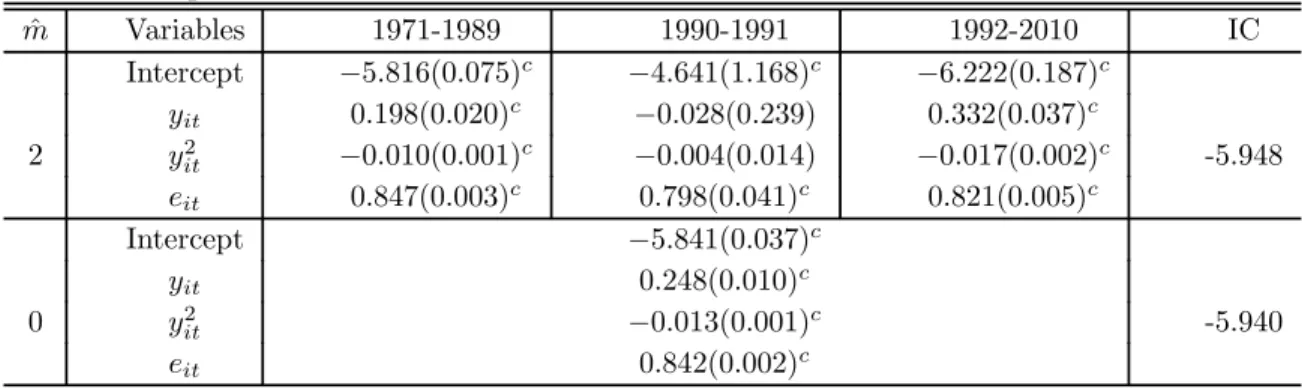
The results are summarized in Table 4. The information criterion defined in (4.2) selects a tuning parameter that identifies two breaks (ˆ = 2) in 1990 and 1992. In thefirst regime of 1971-1990, the EKC hypothesis is confirmed, as the coefficient on the squared income is significantly negative, implying an inverted U-shape. The elasticities of CO2emission per capita with respect
to real income per capita in the regime is(0198−002), where denotes the logarithm of real GDP per capita. The threshold, or the turning points of the EKC, occurs at the per capita income of 19,900 USD. The second regime is a short one, covering only two years, 1990 and 1991. In this regime, the coefficients on both and 2are statistically insignificant. The signs
Table 4: A panel data estimation of the EKC for 74 countries from 1971 to 2010 ˆ Variables 1971-1989 1990-1991 1992-2010 IC Intercept −5816(0075) −4641(1168) −6222(0187) 0198(0020) −0028(0239) 0332(0037) 2 2 −0010(0001) −0004(0014) −0017(0002) -5.948 0847(0003) 0798(0041) 0821(0005) Intercept −5841(0037) 0248(0010) 0 2 −0013(0001) -5.940 0842(0002)
Note. Superscript anddenotes significance level at 10%, 5%, and 1%, respectively. Standard errors are given in parentheses.
of these coefficients do not point to an inverted U-shape. This suggests that, using a short panel or cross-section data set collected in a certain time period, one may reject the EKC hypothesis, while a longer panel data would arrive at the opposite conclusion. In the third regime of 1992-2010, the EKC hypothesis is again confirmed. The elasticities of CO2 emission per capita with
respect to real income per capita in the regime is(0332−0034), implying a threshold of 17,400 USD. Comparing with the first regime, we may conclude that the EKC has shifted leftward in the past two decades. The second regime of 1990-1991 may be regarded as a transition period from the first regime to the second regime, which is more environment-friendly. We also report in Table 4 the case of zero break (ˆ = 0), where coefficients are assumed to be constant. Here the EKC hypothesis is also confirmed, with a threshold at 13,900 USD. Interestingly, the panel data model with constant regression coefficients paints the most optimistic EKC. If we estimate the regression coefficients in the panel data model with two structural breaks detected by the PPC method, however, we see a more cautious picture for the EKC.
6
Conclusions
In this paper, we study the estimation of the panel data models with interactive fixed effects and multiple structural breaks, which substantially generalizes the existing work which either considers the panel models with interactivefixed effects but no structural break (e.g., Bai, 2009), or the panel models with multiple structural breaks but under cross-sectional independence (e.g., Qian and Su, 2015b). We develop a novel PPC estimation procedure with the AGF-LASSO penalty function to consistently estimate both the regression coefficients and the factor loadings.
Under some regularity conditions, we show that both the unknown number of structural breaks and the unobservable break dates can be consistently estimated. In order to further improve the convergence rates, we also estimate the regression coefficients (in different regimes) through the post-LASSO method and then establish the asymptotic distribution theory of the resulting estimators. In particular, the developed shrinkage estimation methodology and the asymptotic theory are also applicable to the case of dynamic panel data. We introduce two data-driven methods to determine the number of factors and choose the tuning parameter involved in the PPC estimation procedure, respectively. The simulation studies show that the proposed PPC method has a high probability of correctly estimating the number of breaks when the structural breaks exist in the simulation design, and a low probability of false detection when there is no structural break. We apply our method to study the EKC for 74 countries over 40 years and
find two breaks in the panel data.
Appendix
Wefirst give in Appendix A some regularity conditions that are used to derive the asymptotic results. Then we provide some technical lemmas and prove the main theoretical results in Appendix B. The proofs of the technical lemmas are given in Appendix C of the supplemental document.
A
Assumptions
We start with the introduction of some notation. Denote = min( √ √) = min( p √) ∆ = min 1≤≤0 ° °0+1−0°° ∆∗ = max 1≤≤0 ° °0+1−0°°
Let =P=1 for1≤ ≤, and ∗=
P =1 for1≤ ≤. Define Ω =Φ −Φ∗ Φ =diag ¡ Φ1 Φ0+1 ¢ Φ∗ =¡Φ∗¢1 ≤≤0+1 where Φ = 1 () 0 −1 X =0 −1 0MΛ0 Φ∗ = 1 () 0 −1 X =0 −1 0 −1 X =0 −1 0MΛ0
() =0−0−1 and =00
¡1
F
00F0¢+0
. In order to prove the asymptotic results stated in Sections 3 and 4, we make the following assumptions.
Assumption 1 (i) There exist two positive definite matrices Σ and ΣΛ such that 1F00F0
→
Σ and 1Λ00Λ0
→ ΣΛ Furthermore, both the common factors 0 and the factor loadings 0 have finite 8-th moments.
(ii) The regressor satisfiesmax1≤≤ kk=
¡ 1212¢, and ≤inf Λ 1min≤≤min ¡ −10MΛ ¢ ≤ max 1≤≤max ¡ −10 ¢ ≤∗
w.p.a.1, where0 ∗∞, and infΛ is taken with respect to Λsuch that 1Λ0Λ=I0.
(iii) Let ε= (1 ) The idiosyncratic error term satisfiesE[] = 0 and E[8] for each and and kεksp=max(√√)where is a bounded positive constant. Furthermore,
max 1≤≤E £ k0k2 ¤ =() max 1≤≤E £ kΛ00k2 ¤ =() E£kΛ00εF0k2¤=( ) max 1≤≤E h° ° X =1 X =1 0 ° °2i =(2) and max 1≤≤E h° ° X =1 X =1 0 ° °2i =(22+4) where can be either 1or0.
(iv) max1≤≤Var() = max1≤≤Var(P=1) =() and there exists 0 such that¯¯E()¯¯≤ andP=1P=12 =(). Furthermore,
max 1≤≤E hX =1 (∗)2i=¡2+ ¢ andEh°° X =1 X =1 00∗0°°2i=¡22¢
Assumption 2 (i)The tuning parametersatisfies that=(1)and0∆− =(1) as (
)→ ∞where is the user-specified positive constant defined in (2.3).
(ii) ∆ → ∞ ∆∗ =(12)and −12+12−12 =(1) as ( )→ ∞
(iii) +1 → ∞ as( )→ ∞
Assumption 3 (i) There exists a positive definite matrix Ω0 such that
°
°Ω −Ω0
° °
=(1)
(ii) There exist0 ≤∗ ∞ such that
0 ≤1≤min≤0+1()≤1≤max≤0+1()≤ ∗
0 (iii)Letting =P=1Λ000,max1≤≤E(2) =(2(+))
(iv) Letting = 1()P 0 −1 =0 −1 0MΛ0( −∗) for = 1 0 + 1 and W =
(10 0 0+1 )0there exist B (3)and Ω1 such that S∗D [W −B (3)]
−→N¡0 S∗Ω1S0∗
¢
whereD is defined in Section 3.2,S∗ is an arbitrary0×(0+ 1)matrix with full row rank,
and 0 is a fixed positive integer.
(v) ( )123 =(1) and =(1)as( )→ ∞.
Assumption 4 As( )→ ∞ 1 →0and 2 1→ ∞
Assumption 5 (i) For any 0≤ 0, there exists a positive constant such that
min T min 0 ∆2 X+1 =1 X−1 =−1 ° °0 − ° °2 ≥
whereα and T are defined in Section 3.2.
(ii) As ( )→ ∞ ∆20
(−12+12−12) =(1)
(iii)As ( )→ ∞ 02 →0 and 2 2 → ∞
Remark A.1. Assumption 1 imposes some standard moment conditions on , 0, 0 and
, which are analogous to those in the existing literature such as Bai and Ng (2002), Bai (2009), Bai and Li (2014), Lu and Su (2015), and Moon and Weidner (2015). As we allow , the dimension of the regression coefficients, to be divergent, some of our moment conditions might be slightly stronger than those in the literature. Assumptions 1(iii) and (iv) allow weak form of cross-sectional dependence and serial dependence among ,0,0 and In partic-ular, unlike Pesaran (2006) and Bai (2009), we do not assume independence between and
( 0 0) for all and our theories are thus applicable to the dynamic autoregressive panel data models with interactive fixed effects. Assumption 2 imposes some mild restrictions on the tuning parameter and the jump sizes of the regression coefficients, which can be easily justified. For example, assuming that the jump sizes are bounded away from zero and infinity and ∼ , Assumption 2 can be simplified to = (1), 0()12 = (1), = (12)
and ()(+1)2 → ∞. Assumption 3 imposes some additional conditions for the proof of the asymptotic distribution theory of the post-LASSO estimation, which can be verified under some primitive conditions. For example, if we assume that { 0} are independent across and for each,{}is a martingale difference sequence with respect to the-field generated by
(−1 1 0−1 10 0) and { } satisfy some strongly mixing conditions, then the moment condition in Assumption 3(iii) holds. Assumption 4 indicates that 1 has to shrink to zero at an appropriate rate to avoid both over-selection and under-selection of the number of factors. Assumptions 5(i)(ii) impose conditions to avoid the selection of model with fewer breaks than the true number by using an information criterion proposed in Section 4.2. Assumption 5(iii) parallels Assumption 4.
B
Proofs of the main asymptotic results
In this appendix, we give the detailed proofs of the asymptotic results in Sections 3 and 4. We start with two technical lemmas whose proofs are provided in Appendix C of the supplemental document.
Lemma B.1 Suppose that Assumption 1 in Appendix A holds and−12+12−12=(1). Let β˙ = (˙01 ˙0)0 be the preliminary estimates of the regression coefficients which mini-mize, ˆ (βΛ), the first term of the objective function defined in (2.4). Then
° °˙ −0 ° ° = ¡ 12−12+−12¢ =
(− 1 ) for any = 12 , where is defined as in
Ap-pendix A.
Lemma B.2 Suppose that Assumption 1 Appendix A holds and let = 1 P=1kˆ−0k2. Then we have (i) 1 P=1(ˆ−0)00MΛˆ=(− 1 12 ), (ii) P=100 Λ00MΛˆ=( −2 +− 1 1 2), and (iii) 1 P=10¡PΛˆ −PΛ0 ¢ = ¡ − 2¢.
We next give the proof of Theorem 3.1 by using the above two lemmas.
Proof of Theorem 3.1. (i) Recall that the penalized estimate of β0 is denoted by βˆ =
¡ˆ
01 ˆ0¢0 and the estimated factor loading matrix is denoted by Λˆ. Note that
−ˆ=(0−ˆ) +Λ00+ (B.1) Then, by (B.1) and using the fact thatMΛ0Λ0 =0, we have
ˆ ¡ˆ βΛˆ¢−ˆ ¡ β0Λ0¢ = 1 X =1 h ˆ ∗ (Λ) + ˆ¦ (Λ)i + X ∈T0 0 ˙ h°°ˆ −ˆ−1°°−°°0−0−1°°i + X ∈T ˙ h°°ˆ −ˆ−1°°−°°0 −0−1°°i (B.2) where ˆ ∗ (Λ) = 1 h¡ˆ −0¢00MΛˆ ¡ˆ −0¢−2¡ˆ−0¢00MΛˆΛ 00 +00Λ00MΛˆΛ 00 i ˆ ¦ (Λ) = 1 h −2¡ˆ−0¢00MΛˆ+ 200Λ00MΛˆ−0PΛˆ+0PΛ0 i
As 0−0−1 =0 for∈T, the last term on the right hand side of (B.2) satisfies that X ∈T ˙ h°°ˆ−ˆ−1 ° °−°°0−0−1°°i= X ∈T ˙ ° °ˆ −ˆ−1 ° °≥0 (B.3)
By the triangle inequality, the Cauchy-Schwarz inequality, Lemma B.1 and Assumption 2(ii) in Appendix A, we can prove that
X ∈T0 0 ˙ h°°ˆ −ˆ−1°°−°°0 −0−1°°i ≤ (∆− ) X ∈T0 0 ° °ˆ −0 ° ° ≤ (∆− )(0)12 ⎛ ⎜ ⎝ X ∈T0 0 ° °ˆ −0 ° °2 ⎞ ⎟ ⎠ 12 ≤ (∆− )( 0)12 Ã 1 X =1 ° °ˆ −0 ° °2 !12
Note that Assumption 2(i) implies that(0)12−12∆ − =(− 1 )where = min(
p
√
). This, together with the above argument, indicates that X ∈T0 0 ˙ h°°ˆ −ˆ−1°°−°°0−0−1°°i=(− 1 12 ) (B.4)
By Lemma B.2, we can readily show that
1 X =1 ˆ ¦ (Λ) = ³ − 2 + −1 1 2´ (B.5) Combining (B.4) and (B.5), we have
ˆ ¡βˆΛˆ¢−ˆ ¡β0Λ0¢≥ 1 X =1 ˆ ∗ (Λ) + ³ − 2 + −1 1 2´ (B.6) Define the vectors: ˆ d = ˆβ−β0 anddˆΛ = 1 12vec(MΛˆΛ 0)
wherevec(·) denotes the vectorization of a matrix; and define the matrices:
ˆ A = 1 diag ¡ 10MΛˆ1 0 MΛˆ ¢ Bˆ = (F00F0)⊗I and ˆ C = 1 12 £ 10⊗MΛˆ1 0 ⊗MΛˆ ¤
where⊗ denotes the Kronecker product. It is easy to verify that 1 X =1 ¡ˆ −0¢00MΛˆ ¡ˆ −0¢= 1 dˆ 0 Aˆdˆ 1 X =1 ¡ˆ −0¢00MΛˆΛ00= 1 X =1 TrnMΛˆΛ00 ¡ˆ −0¢00MΛˆ o = 1 ˆ d0ΛCˆdˆ 1 X =1 00Λ00MΛˆΛ00 = 1 X =1 Tr³MΛˆΛ0000Λ00MΛˆ ´ = 1 dˆ 0 ΛBˆdˆΛ
where we have used the following facts on matrix calculation: Tr¡A1A2A3
¢ =vec0¡A1 ¢¡ A2 ⊗ I ¢ vec¡A3 ¢ and Tr¡A1A2A3A4 ¢ = vec0¡A1 ¢¡ A2 ⊗A04 ¢
vec¡A03¢ with being the size of the column vectors inA3. Using the above notations, we may show that
1 X =1 ˆ ∗ (Λ) = 1 ¡ˆ d0Aˆdˆ−2ˆd 0 ΛCˆdˆ+ ˆd 0 ΛBˆdˆΛ ¢ = 1 ¡ˆ d0Dˆdˆ+ ˆd 0 ∗Bˆdˆ∗ ¢ (B.7) whereDˆ = ˆA−Cˆ0Bˆ+Cˆ andˆd∗= ˆdΛ−Bˆ +ˆ
Cdˆ. By Assumption 1(i), we may show that the min-imum eigenvalue of 1Bˆ is bounded away from zero w.p.a.1, i.e., there exists a positive constant 1such thatmin
¡ˆ
B¢ 1for sufficiently large. We next show thatmax
¡ˆ
C0Cˆ¢=(1). Letting =000, it is easy to verify that
ˆ C0Cˆ = 1 ⎛ ⎜ ⎜ ⎜ ⎜ ⎜ ⎝ 1110MΛˆ1 1210MΛˆ2 110MΛˆ 2120MΛˆ1 2220MΛˆ2 220MΛˆ .. . ... . .. ... 10MΛˆ1 20MΛˆ2 0 MΛˆ ⎞ ⎟ ⎟ ⎟ ⎟ ⎟ ⎠ Letting ˆ C1= 1 ⎛ ⎜ ⎜ ⎜ ⎜ ⎜ ⎝ 1110MΛˆ1 1210MΛˆ2 110MΛˆ 0 2220MΛˆ2 220MΛˆ .. . ... . .. ... 0 0 0MΛˆ ⎞ ⎟ ⎟ ⎟ ⎟ ⎟ ⎠ and Cˆ= 1diag ¡ 1110MΛˆ1 0 MΛˆ¢, we have ˆ C0Cˆ = ˆC1+ ˆC01−Cˆ (B.8) By the fact that the eigenvalues of a block upper/lower triangular matrix are the combined eigenvalues of its diagonal block matrices, Weyl’s inequality, and Assumptions 1(i) and (ii), we
have
−1max( ˆC0Cˆ) ≤ −1{2max( ˆC1)−min( ˆC)} ≤ 2−1 max 1≤≤ ° °0°°2max¡−10MΛˆ ¢ = (−1)(14)(1) =(−34) where we use the fact that max1≤≤k0k2 =
¡
14¢ by Assumption 1(i) and the Markov inequality. On the other hand, we note that the minimum eigenvalue of Aˆ is positive and bounded away from zero w.p.a.1. Hence, the matrixDˆ is asymptotically positive definite as its minimum eigenvalue is positive and bounded away from zero w.p.a.1 by using the above facts. Then, by (B.7) and (B.8), we can readily show that there exist two positive constants2 and3
such that 2 k ˆ dk2+3kdˆ∗k2≤ 1 X =1 ˆ ∗ (Λ) (B.9) which indicates that
2 k ˆ dk2+3kˆd∗k2+ ¡ − 2 +− 1 1 2¢≤ˆ ¡ˆ βΛˆ¢−ˆ ¡ β0Λ0¢ (B.10) Multiplying both sides of (B.10) by 2 and noting that 1kˆdk2 = and ˆ
¡ˆ
βΛˆ¢− ˆ
¡
β0Λ0¢≤0, we readily show that
22 +(1) +(1)·
£
2 ¤12≤0 (B.11) When2 is sufficiently large, thefirst term on the left hand side of (B.11) would dominate the other two terms, which would lead to a contradiction. Hence, we must have that2 is stochastically bounded, implying that =¡−1+−1¢This completes the proof of Theorem 3.1(i).
(ii)The proof for the point-wise convergence result is similar to the proof of Theorem 3.2(ii) in Qian and Su (2015b), where the condition 0∆− =(1) in Assumption 2(i) is used to handle the penalty term. We omit the details to save space.
We have thus completed the proof of Theorem 3.1. ¥
Proof of Theorem 3.2. To prove the sparsity, it is equivalent to showing
P¡°°ˆ
°
°6= 0for some ∈T¢→0 (B.12) as( )→ ∞. We consider two cases: (i) 2≤≤−1and ∈T; and (ii)= and ∈T. Recall that = min(−1212 12)