KRANNERT SCHOOL OF
MANAGEMENT
Purdue
University
West
Lafayette,
Indiana
Testing for Multiple Structural Changes in Cointegrated
Regression Models
By
Mohitosh Kejriwal
Pierre Perron
Paper No. 1216
Date: November 2008
Institute for Research in the
Behavioral, Economic, and
Management Sciences
Testing for Multiple Structural Changes in
Cointegrated Regression Models
∗
Mohitosh Kejriwal†
Purdue University
Pierre Perron‡
Boston University
August 30, 2007; Revised November 20, 2008
Abstract
This paper considers issues related to testing for multiple structural changes in cointegrated systems. We derive the limiting distribution of the Sup-Wald test under mild conditions on the errors and regressors for a variety of testing problems. We show that even if the coefficients of the integrated regressors are held fixed but the intercept is allowed to change, the limit distributions are not the same as would prevail in a stationary framework. Including stationary regressors whose coefficients are not allowed to change does not affect the limiting distribution of the tests under the null hypothesis. We also propose a procedure that allows one to test the null hypothesis of, say, k changes, versus the alternative hypothesis of k+ 1changes. This sequential procedure is useful in that it permits consistent estimation of the number of breaks present. We show via simulations that our tests maintain the correct size in finite samples and are much more powerful than the commonly used LM tests, which suffer from important problems of non-monotonic power in the presence of serial correlation in the errors.
Keywords: Change-point, Sequential procedure, Wald tests, Unit Roots, Cointe-gration.
JEL Classification: C22
∗Perron acknowledgesfinancial support for this work from the National Science Foundation under Grant
SES-0649350. We are grateful to an Associate Editor and two referees for useful suggestions. One referee was especially helpful in pointing out an error in a previous version.
†Krannert School of Management, Purdue University, 403 West State Street, West Lafayette IN 47907
1 Introduction
Issues related to structural change have received a considerable amount of attention in the statistics and econometrics literature. Andrews (1993) and Andrews and Ploberger (1994) provide a comprehensive treatment of the problem of testing for structural change assuming that the change point is unknown. Bai (1997) studies the least squares estimation of a single change point in regressions involving stationary and/or trending regressors. He derives the consistency, rate of convergence and the limiting distribution of the change point estimator under general conditions on the regressors and the errors. Perron and Zhu (2005) analyze the properties of parameter estimates in models where the trend function exhibits a slope change at an unknown date and the errors can be either stationary, I(0), or have a unit root, I(1), where here, and throughout the text, we refer to an I(0) process as one whose partial sums satisfies a Functional Central Limit Theorem with a Brownian motion as the limit random variable, and an I(1) as the partial sums of an I(0)series.
With integrated variables, the case of interest is when the variables are cointegrated. Accounting for parameter shifts is crucial in cointegration analysis since it normally involves long spans of data which are more likely to be affected by structural breaks. Bai, Lumsdaine and Stock (1998) consider a single break in a multi-equations system. They show consis-tency of the maximum likelihood estimates and obtain a limit distribution of the break date estimate under a shrinking shifts scenario. Kejriwal and Perron (2008b) study the proper-ties of the estimates of the break dates and parameters in a linear regression with multiple structural changes involving I(1),I(0) and trending regressors.
With respect to testing, Hansen (1992b) develops tests of the null hypothesis of no change in cointegrated models where all coefficients are allowed to change. An extension to partial changes has been analyzed by Kuo (1998). The tests considered are the Sup and Mean LM tests directed against an alternative of a one time change in parameters. Hao (1996) also suggests the use of the exponential LM test. Seo (1998) considers the Sup, Mean and Exp versions of the LM test within a cointegrated VAR setup. However, these test procedures are based on the fully modified estimation method (Phillips and Hansen, 1990) which has been shown to lead to tests with very poorfinite sample properties (Carrion-i-Silvestre and Sansó-i-Rosselló, 2006). The results in Quintos and Phillips (1993) also suggest that the LM tests are likely to suffer from the problem of low power in finite samples. Moreover, simulation experiments in Hansen (2000) show that the LM test is quite poorly behaved in the presence of structural changes in the marginal distribution of the regressors. On the
other hand, the Sup-Wald test is shown to be reasonably robust to such shifts. Hansen (2003) considers multiple structural changes in a cointegrated system, though his analysis is restricted to the case of known break dates. Finally, Qu (2007) proposes a procedure to detect whether cointegration is present when the cointegrating vector changes at some unknown possibly multiple dates.
The literature on testing for multiple structural changes is relatively sparse. It is, however, practically important since single break tests can suffer from non-monotonic power when the alternative involves more than one break. As stressed by Perron (2006), most tests may exhibit non-monotonic power functions if the number of breaks present is greater than the number explicitly accounted for in the construction of the tests. The aim of this paper is to provide a comprehensive treatment of issues related to testing for multiple structural changes occurring at unknown dates in cointegrated regression models. Our work builds on Bai and Perron (1998) who undertake a similar treatment in a stationary context. Our framework is general enough to allow both I(0) and I(1) variables in the regression. The assumptions about the distribution of the error processes are mild enough to allow for general forms of serial correlation. Moreover, we analyze both pure and partial structural change models. A partial change model is useful in allowing potential savings in the number of degrees of freedom, an issue particularly relevant for multiple changes. It is also important in empirical work since it helps to isolate the variables which are responsible for the failure of the null hypothesis. We derive the limiting distribution of the sup-Wald test under the null hypothesis of no structural change against the alternative hypothesis of a given number of cointegrating regimes. We also consider the double maximum tests proposed in Bai and Perron (1998). We provide critical values for a wide variety of models that are relevant in practice. Our asymptotic results have important implications for inference. We show that in models with both I(1) and I(0) variables, inference is possible as long as the intercept is allowed to change across regimes. Otherwise, the limiting distributions of the tests depend on nuisance parameters. Finally, our simulation experiments show that with serially correlated errors, the commonly used Sup, Mean and Exp-LM tests suffer from non-monotonic power problems. This is true for cases with a single break as well as with multiple breaks. We propose a modified sup Wald test that exhibits a power function which is monotonic with respect to the magnitude of the break(s) while maintaining reasonable size properties.
The paper is organized as follows. Section 2 presents the model and assumptions. In Section 3, we describe the testing problems and the test statistics used. Section 4 contains the theoretical results of this paper about the limit distributions of the tests for a wide variety
of cases. This isfirst done for models involving non-trending regressors, no serial correlation in the errors and exogenous regressors. These restrictions are relaxed in Section 4.2, 5.1 and 5.2, respectively. Asymptotic critical values are presented in Section 4.3. Section 6 presents simulation experiments that address issues related to the size and power of the tests including a comparison with the often used LM tests. Section 7 offers concluding remarks and all technical derivations are included in a mathematical appendix.
2 The model and assumptions
Consider the following linear regression model with m breaks (m+ 1 regimes):
yt=cj +zf t0 δf +zbt0 δbj+x0f tβf +x0btβbj+ut (t=Tj−1+ 1, ..., Tj) (1)
for j = 1, ..., m+ 1, where T0 = 0, Tm+1 =T and T is the sample size. In this model, yt is
a scalar dependent I(1) variable, xf t (pf ×1) and xbt (pb×1) are vectors of I(0) variables
while zf t (qf ×1) andzbt (qb×1)are vectors ofI(1) variables defined by: zf t =zf,t−1+ufzt,
zbt = zb,t−1 +ubzt, xf t = μf +u f
xt and xbt = μb +uxtb , where zf0 and zb0 are assumed, for simplicity, to be eitherOp(1)random variables orfixedfinite constants. For ease of reference,
the subscript b on the error term stands for “break” and the subscript f stands for “fixed” (across regimes). The break points (T1, ..., Tm) are treated as unknown. This is a partial
structural change model in which the coefficients of only a subset of the regressors are subject to change. When pf =qf = 0, we have a pure structural change model with all coefficients
allowed to change across regimes. It will be useful to express (1) in matrix form as: Y =Gα+ ¯W γ+U
where Y = (y1, ..., yT)0, G = (Zf, Xf), Zf = (zf1, ..., zf T)0, Xf = (xf1, ..., xf T)0, U =
(u1, ..., uT)0, W = (w1, ..., wT)0, wt = (1, zbt0 , x0bt)0, γ = (δ0b1, β0b1, ..., δ0b,m+1, β0b,m+1)0, α =
(δ0f, β0f)0 and W¯ is the matrix which diagonally partitionsW at them−partition(T
1, ..., Tm),
that is, W¯ =diag(W1, ..., Wm+1) with Wi = (wTi−1+1, ..., wTi)0 for i = 1, ..., m+ 1. Kejriwal
and Perron (2008b) analyze the properties of the estimates of the break dates and the other parameters of the model under general conditions on the regressors and the errors. In this paper, the interest is in testing the null hypothesis of no structural change versus the alter-native hypothesis of m changes as specified by the model (1). Hence, the data generating process is assumed to be given by (1) with pb =qb = 0.
As a matter of notation, “→p ” denotes convergence in probability, “→d” convergence in distribution and “⇒” weak convergence in the space D[0,1] under the Skorohod metric.
Also, xt = (x0f t, x0bt)0, uxt = (ufxt0, ubxt0)0, zt = (zf t0 , z0bt)0, μ = (μ0f, μ0b)0 and λ = {λ1, ..., λm} is
the vector of break fractions defined byλi = Ti/T for i = 1, ..., m. We make the following
assumptions onξt= (ut, ufzt0, ubzt0, u f0
xt, ubxt0)0, a vector of dimension n=qf +pf +qb+pb+ 1.
Assumption A1: The vectorξtsatisfies the following multivariate Functional Central Limit
Theorem (FCLT):T−1/2P[T r]
t=1 ξt ⇒B(r), withB(r) = (B1(r), Bfz(r)0, Bzb(r)0, Bxf(r)0, Bxb(r)0)0is
a nvector Brownian motion with symmetric covariance matrix
Ω = ⎛ ⎜ ⎜ ⎜ ⎜ ⎜ ⎜ ⎜ ⎜ ⎜ ⎝ σ2 Ωf 1z Ωb1z Ω f 1x Ωb1x Ωfz1 Ωf f zz Ωf bzz Ωf bzx Ωf fzx Ωb z1 Ωbfzz Ωbbzz Ωbfzx Ωbbzx Ωfx1 Ωf fxz Ωf bxz Ωf fxx Ωf bxx Ωb x1 Ωbfxz Ωbbxz Ωbfxx Ωbbxx ⎞ ⎟ ⎟ ⎟ ⎟ ⎟ ⎟ ⎟ ⎟ ⎟ ⎠ 1 qf qb pf pb = lim T→∞T −1E(S TST0 ) =Σ+Λ+Λ0 whereST = PT t=1ξt,Σ= limT→∞T−1 PT t=1E(ξtξ0t)andΛ= limT→∞T−1 PT−1 j=1 PT−j t=1 E(ξtξ0t+j).
We also assume σ2 >0 andplim
T→∞T−1
PT
t=1u2t = limT→∞T−1
PT
t=1E[u2t]≡σ2u.
Assumption A2: The vector {xtut} satisfies Assumption A4 in Qu and Perron (2007) so
that T−1/2P[tT r=1](uxtf , ubxt)ut ⇒ σQ∗1/2Wx∗(r), where Wx∗(r) = (Wxf∗ (r)0, Wxb∗(r)0)0 is a (pf +
pb) vector of independent Wiener processes and
Q∗ = ⎡ ⎣ Qf fx ∗ Qf bx ∗ Qbf∗ x Qbbx∗ ⎤ ⎦
Assumption A3: For alltands: a)E(uxtutzs) = 0; b)E(uxtutus) = 0; c)E(uxtutuxs) = 0.
Assumption A4: The matrix
⎛ ⎝Ω f f zz Ωf bzz Ωbf zz Ωbbzz ⎞ ⎠ is positive definite. Assumption A5: T−1P[T s] t=1xtx0t p → sQ and, T−1P[T s] t=1 uxtu0xt p → sQ∗, uniformly in s ∈
[0,1], for some positive definite matricesQ andQ∗.
Assumption A1 requires that the errors satisfy a multivariate FCLT. The conditions for this to hold are very general (see, e.g., Davidson, 1994). It can be shown to apply to a large class of linear processes including those generated by all stationary and invertible ARMA models. A2 guarantees that a F CLT also holds for the sequence {uxtut}. Assumption A3
restricts somewhat the class of models applicable but is quite mild. Sufficient conditions for it to hold are: for (a) that the I(0) regressors are uncorrelated with the errors contempo-raneously even conditional on the I(1) variables; for (b) that the autocovariance structure
of the I(0) regressors be independent of the errors and, similarly, for (c) that the autoco-variance structure of the errors be independent of the I(0) regressors. This assumption is needed to guarantee thatW∗
x(·)andB(·)are uncorrelated and, being Gaussian, are therefore
independent. Without this condition, the analysis would be much more complex. A4 rules out cointegration among theI(1)regressors. A5 is standard forI(0)regressors but rules out trending regressors, which we shall relax in Section 4.2.
Under the alternative hypothesis, the estimates of the parameters are obtained by min-imizing the global sum of squared residuals. For each m-partition (T1, ..., Tm), denoted {Tj}, the associated least squares estimates ofα andγ are obtained by minimizing
SSRT(T1, ..., Tm) = mP+1 i=1 Ti P t=Ti−1+1 [yt−ci−zf t0 δf −xf t0 βf −zbt0 δbi−x0btβbi] 2 (2)
Let αˆ({Tj}) and ˆγ({Tj}) be the resulting estimates. Substituting these into the objective
function and denoting the resulting sum of squared residuals asST(T1, ..., Tm),the estimate
of the break points are( ˆT1, ...,Tˆm) = arg min T1,...,TmST(T1, ..., Tm), where the minimization is
taken over all partitions(T1, ..., Tm)such thatTi−Ti−1 ≥ T for some >0. The estimates of the regression coefficients are thenαˆ = ˆα({Tˆj})andˆγ = ˆγ({Tˆj}). Such estimates can be
ob-tained using the algorithm of Bai and Perron (2003). Finally, consistent estimates of the ma-tricesΣandΛ(and, hence,Ω) areΣˆ =T−1PT
t=1ˆξtˆξ 0 tandΛˆ =T−1 PT−1 j=1 w(j/l) PT−j t=1 ˆξtˆξt+j,
whereˆξt= (ˆut,∆zf t0 ,∆zbt0 ,(xf t−x¯f)0,(xbt−x¯b)0)0 withuˆt the OLS residuals from regression
(1), x¯i =T−1
PT
t=1xit (i =f, b) and w(j/l)is a kernel function that is continuous and even
withw(0) = 1andR−∞∞ w2(x)dx <∞. Also,l → ∞asT → ∞andl =o(T1/2). Consistency
of these covariance matrix estimates has been shown in Hansen (1992c).
3 The testing problem and the test statistics
The data generating process (1) is the most general and in practice restricted versions may be used. This gives rise to a variety of possible cases for the testing problems considered. We classify them in two categories: a) models with only I(1) regressors; b) models with bothI(1) andI(0)regressors. This classification in two categories is useful since oftentimes researchers are faced with only I(1) variables. For this category (a), the testing problems considered are the following (for ease of reference, we list the relevant regression under the alternative hypothesis):
Testing problems, Category (a), Models with I(1) variables only (pf =pb = 0, for
all cases): LetHa
1. Ha
0(1) ={H0a, qf = 0} versus H1a(1) ={qf = 0} (yt=cj +zbt0 δbj+ut);
2. Ha
0(2) ={H0a, qb = 0} versus H1a(2) ={qb = 0} (yt=cj +zf t0 δf +ut);
3. Ha
0(3) = {H0a, qf = 0} versus H1a(3) = {cj = c for all j = 1, .., m+ 1, qf = 0}
(yt =c+z0btδbj+ut);
4. H0a(4) ={H0a} versusH1a(4) ={no restriction} (yt=cj +z0f tδf +z0btδbj+ut);
5. Ha
0(5) ={H0a}versusH1a(5) ={cj =cfor allj = 1, .., m+1}(yt =c+z0f tδf+zbt0 δbj+ut).
Testing problems, Category (b), Models with both I(1) and I(0) variables: Let
H0b denotes the restrictions {cj =c, δbj =δb, βbj =βb for all j = 1, .., m+ 1}.
1. Hb
0(1) ={H0b, pf =qb = 0} versusH1b(1) ={cj =cfor all j = 1, .., m+ 1,pf =qb = 0}
(yt =c+z0f tδf +x0btβbj+ut);
2. H0b(2) ={H0b, pb =qf = 0} versusH1b(2) ={cj =cfor all j = 1, .., m+ 1,pb =qf = 0}
(yt =c+z0btδbj+x0f tβf +ut);
3. Hb
0(3) ={H0b,pf =qf = 0}versusH1b(3) ={cj =cfor allj = 1, .., m+ 1,pf =qf = 0}
(yt =c+z0btδbj+x0btβbj+ut); 4. Hb 0(4) ={H0b,pf =qf = 0}versusH1b(4) ={pf =qf = 0}(yt =cj+zbt0 δbj+x0btβbj+ut); 5. Hb 0(5) ={H0b,pb =qb = 0}versus H1b(5) ={pb =qb = 0}(yt =cj+zf t0 δf+x0f tβf+ut); 6. Hb 0(6) ={H0b,pb =qf = 0}versusH1b(6) ={pb =qf = 0}(yt=cj+zbt0 δbj+x0f tβf+ut); 7. H0b(7) ={H0b,pf =qb = 0}versusH1b(7) ={pf =qb = 0}(yt=cj+zf t0 δf+x0btβbj+ut); 8. H0b(8) ={H0b, qf = 0} versusH1b(8) ={qf = 0}(yt=cj+zbt0 δbj+xf t0 βf +x0btβbj+ut); 9. Hb 0(9) ={H0b, qb = 0} versus H1b(9) ={qb = 0} (yt=cj +zf t0 δf +x0f tβf +x0btβbj+ut); 10. Hb 0(10) = {H0b} versus H1b(10) = {no restriction} (yt = cj +zf t0 δf +zbt0 δbj +x0f tβf + x0 btβbj+ut); 11. Hb
0(11) = {H0b} versus H1b(10) = {cj = c for all j = 1, .., m+ 1} (yt = c+zf t0 δf +
z0
We now give a brief description of each of the models in the two categories. First consider Category (a). Case 1 is a pure structural change model which allows for a change in the intercept as well. Case 2 is a partial change model in which only the intercept is allowed to change. Case 3 is again a partial change model where the intercept is not allowed to change. Cases 4 and 5 are block partial models in which a subset of the I(1) coefficients is allowed to change. In Category (b), Cases 1 to 3 are partial change models where the intercept is not allowed to change across regimes. Case 4 is a pure change model where all I(1) and I(0) coefficients as well as the intercept are allowed to change. Case 5 is a partial change model, which involves only an intercept shift. Case 6 is a partial change model where the I(0) coefficients are not allowed to change. Similarly, Case 7 is a partial change model where theI(1)coefficients are not allowed to change. Cases 8-11 are block partial models in which a subset of coefficients of at least one type of regressor is not allowed to change.
We consider three types of tests. Thefirst applies when the alternative hypothesis involves afixed valuem =kof changes. We consider the Wald test, scaled by the number of regressors whose coefficient are allowed to change, defined by
FT(λ, k) = ( T −(k+ 1)(qb+pb)−(pf +qf) k ) ˆ γ0R0(R( ¯W0M GW¯)−1R0)−1Rγˆ SSRk (3) where R is the conventional matrix such that (Rγ)0 = (γ0
1 −γ02, ..., γ0k−γ0k+1) and MG =
I−G(G0G)−1G0. HereSSRkis the sum of squared residuals under the alternative hypothesis.
As in Bai and Perron (1998), we define the following set for some arbitrary small positive number ,Λk={λ :|λi+1−λi|≥ , λ1 ≥ , λk ≤1− }. The sup-Wald test is then defined
as sup-FT(k) = supλ∈ΛkFT(λ, k). Since, in the current cases, the estimates λˆ ={λˆ1, ...,λˆk}
with ˆλi = ˆTi/T (for i= 1, ..., k) obtained by minimizing the global sum of squared residuals
correspond to those that maximize the test FT(λ, k), we have sup-FT(k) =FT(ˆλ, k).
The second procedure applies when the alternative hypothesis involves an unknown num-ber of changes between1and some upper boundM. As in Bai and Perron (1998), we consider a double maximum test based on the maximum of the individual tests for the null of no break versus mbreaks(m= 1, ..., M), defined byU DmaxFT(M) = max1≤m≤M supλ∈ΛmFT(λ, m).
This test is arguably the most useful to apply when trying to determine if structural changes are present. Simulations presented in Bai and Perron (2006) show that with multiple changes, the power of tests for a single break can be quite low in finite samples, especially for cer-tain types of multiple changes; e.g., two breaks with identical first and third regimes. Also tests for a particular number of changes may have non-monotonic power when the number of changes is greater than specified. Finally, in their simulations they found the power of
U Dmaxto be nearly as high as that of thesup-FT test based on the true number of changes.
The third testing procedure is a sequential one based on the estimates of the break dates obtained from a global minimization of sum of squared residuals, as in Bai and Perron (1998). Consider a model with k breaks, with estimates denoted by ( ˆT1, ...,Tˆk), which are obtained
by a global minimization of the sum of squared residuals. The procedure to test the null hypothesis ofk breaks versus the alternative hypothesis ofk+ 1 breaks is to perform a one break test for each of the(k+ 1)segments defined by the partition ( ˆT1, ...,Tˆk) and to assess
whether the maximum of the tests is significant. More precisely, the test is defined by
SEQT (k+ 1|k) = max
1≤j≤k+1τsup∈Λj,εT{SSRT( ˆT1, ...,
ˆ
Tk)−SSRT( ˆT1, ...Tˆj−1, τ ,Tˆj, ...,Tˆk)}/SSRk+1
where Λj,ε = {τ; ˆTj−1+ ( ˆTj −Tˆj−1)ε ≤ τ ≤ Tˆj −( ˆTj −Tˆj−1)ε}. Note that this is different from a purely sequential procedure since for each value ofk the break dates are re-estimated to get those that correspond to the global minimizers of the sum of squared residuals.
4 The asymptotic distributions of the tests
With integrated regressors, an important issue that arises is the correlation between the regressors and the errors. We first consider the case where all I(1) regressors are strictly exogenous. Later, we deal with the case of endogenous regressors and show that if the regression is augmented with leads and lags of the thefirst differences of theI(1) regressors, the limiting distribution of the tests is the same as that obtained when all I(1) regressors are strictly exogenous. Hence, for now, we assume Ωf1z = Ωb
1z = 0, which will be relaxed in
Section 5.2. We also start with the following assumption that imposes serially uncorrelated errors in the cointegrating regression to be relaxed in Section 5.1:
Assumption A6: Let ξ∗t = (ufzt0, ubzt0, u f0
xt, ubxt0)0, the errors {ut} form an array of martingale
differences relative to{Ft}=σ-field{ξt∗−s, ut−1−s;s >0}.
4.1 The main theoretical results
As a matter of notation, we define the following functionals, where W1 =σ−1B1: h(G, a, b) = (RabGdW1)0( Rb aGG0)− 1(Rb aGdW1), f(G) = ( kP+1 i=1 Rλi λi−1GdW1) 0(kP+1 i=1 Rλi λi−1GG 0)−1(kP+1 i=1 Rλi λi−1GdW1),
g(G, a, b) = (aG(b) − bG(a))0(aG(b) − bG(a))/ba(b − a) and G(a,b)(r) = G(r)
− (λb −
λa−1)−1
Rλb
λa−1G. Also, by convention λ0 = 0 and λk+1 = 1. The limit distributions of
the tests when only I(1)variables are involved are stated in the following Theorem.
Theorem 1 Assume A1-A6 and Ωf1z =Ωb1z = 0. For the testing problems in Category (a),
the limit distribution ofsupλ∈ΛkFT(λ, k)issupλ∈ΛkF(λ, k)/k with F(λ, k)defined as follows
for the various cases. For Case (1),
F(λ, k) =
k
P
i=1
[h(Wzb(1,i),0, λi)−h(Wzb(1,i+1),0, λi+1) +h(Wzb(i+1,i+1), λi, λi+1) +g(W1, λi, λi+1)]
For Case (2),F(λ, k) =f(Wzf(i,i))−h(Wzf(1,k+1),0,1) +Pki=1g(W1, λi, λi+1), whereWzf(r) =
(Ωf fzz)−1/2Bzf(r). For Case (3), F(λ, k) =f(Pzib)−h(Wzb(1,k+1),0,1)−W1(1)2+ kP+1 i=1 h(Wzb, λi−1, λi) where Pzib(r) = 1−( Rλi λi−1W b0 z )( Rλi λi−1W b zWb 0
z )−1Wzb(r), for r ∈[λi−1, λi]. For Case (4),
F(λ, k) =f(WzM(i,i))−h(Wzf b(1,k+1),0,1) + kP+1 i=1 h(Wzb(i,i), λi−1, λi) + k P i=1 g(W1, λi, λi+1) with Wf b z (r) = (Wzf(r), Wzb(r)), and where WzM(i,i)(r) =Wzf(i,i)(r)−Rλi λi−1W f(i,i) z W b(i,i)0 z ( Rλi λi−1W b(i,i) z W b(i,i)0 z )− 1Wb(i,i) z (r). For Case (5), F(λ, k) =f(Pzi)−h(W f b(1,k+1) z ,0,1)−W1(1)2+ Pk+1 i=1 h(W b z, λi−1, λi), where Pzi(r)0 = (Pzib(r)0, P f b zi(r)0) with P f b zi(r) =Wzf(r)−( Rλi λi−1W f zWzb0)( Rλi λi−1W b zWb 0 z )−1Wzb(r).
Theorem 1 shows that it is possible to make inference in models involving I(1)variables using the sup-Wald test. Also, the limiting distributions are different depending on whether the intercept and/or the I(1) coefficients are allowed to change. Note that for Cases 2, 4 and 5 the limit distributions depend on the number ofI(1)coefficients that are not allowed to change. This is different from a stationary framework where the limit distribution is independent of the number of regressors whose coefficients are not allowed to change. We now consider the limit distributions of the test for the various cases in Category (b) where both I(1) and I(0) regressors are present.
Theorem 2 Assume A1-A6 and Ωf1z = Ωb
1z = 0 and let Wxb∗(1) = (Wxb∗0, W1)0. For cases
are given by supλ∈ΛkF(λ, k)/k with F(λ, k) defined as follows. For case (1), F(λ, k) =
Pk
i=1g(Wxb∗, λi, λi+1). For Case (2), the limit distribution is the same as for Case (3) in
Category (a). For Case (3),
F(λ, k) =f(Pzib)−h(Wzb(1,k+1),0,1)−W1(1)2+ kP+1 i=1 h(Wzb, λi−1, λi) + k P i=1 g(Wxb∗, λi, λi+1).
For Cases (4) and (8),
F(λ, k) =
k
P
i=1
[h(Wzb(1,i),0, λi)−h(Wzb(1,i+1),0, λi+1)+h(Wzb(i+1,i+1), λi, λi+1)+g(Wxb∗(1), λi, λi+1)]
For Cases (5) and (6), the limit distributions are the same as for Cases (2) and (1), respec-tively, in Category (a). For Case (7) and (9),
F(λ, k) =f(Wzf(i,i))−h(Wzf(1,k+1),0,1) + k P i=1 g(Wxb∗(1), λi, λi+1). For Case (10), F(λ, k) =f(WzM(i,i))−h(Wzf b(1,k+1),0,1) + kP+1 i=1 h(Wzb(i,i), λi−1, λi) + k P i=1 g(Wxb∗(1), λi, λi+1).
And, for Case (11),
F(λ, k) =f(Pzi)−h(Wzf b(1,k+1),0,1)−W1(1)2 + kP+1 i=1 h(Wzb, λi−1, λi) + k P i=1 g(Wxb∗, λi, λi+1).
The practical implications of Theorem 2 are as follows. As shown in Case (1), if the intercept and the I(1)variables are heldfixed and only the coefficients on the I(0)variables are allowed to change, the same limit distribution as in Bai and Perron (1998) applies. However, this equivalence with the case of stationary regressors only holds if the constant is not allowed to change. As shown in Case (7), the limit distribution is different when the intercept is allowed to change and depends on the number of I(1) variables present. The effect of allowing the intercept to change or not can also be seen by comparing Cases (3) and (4). The limit distributions are different and, as expected, both depend on the number of I(1) and I(0) variables whose coefficients are allowed to change. A similar feature also applies when the regression involvesI(1)andI(0)variables whose coefficients are not allowed to change, as shown in Cases (10) and (11). Comparing these with Cases (3) and (4) again shows that havingI(1)variables whose coefficients are not allowed to change alters the limit distributions. Finally, comparing Cases (a-1) and (b-6), (a-2) and (b-5), (a-3) and (b-2), (b-4) and (b-8), and (b-7) and (b-9), shows that includingI(0)regressors whose coefficients are not allowed to change does not alter the limit distribution.
Remark 1 For Case (4) in Category (b), the limit distribution of supλ∈ΛkFT(λ, k) is: sup (λ1,...,λ k)∈Λk { k P i=1 (S∗(λi, λi+1)0V(λi, λi+1)−1S∗(λi, λi+1)) + k P i=1 (λiWxb∗(λi+1)−λi+1Wxb∗(λi))0(λiWxb∗(λi+1)−λi+1Wxb∗(λi)) λi+1λi(λi+1−λi) } withS∗(λ i, λi+1) =S(λi)−M(λi)M(λi+1)−1S(λi+1),V(λi, λi+1) =M(λi)−M(λi)M(λi+1)−1M(λi), S(λi) = Rλi 0 Z∗dW1, M(λi) = Rλi 0 Z∗Z∗0 and Z∗ = (1, W b0
z )0. The first summation
corre-sponds to the distribution in Case 1 of Category (a), while the second correcorre-sponds to the
pb I(0) regressors whose coefficients are allowed to change.
With these theoretical results for the sup-FT(λ, k), we can obtain the limit distribution
of theU Dmax andSEQT(k+ 1|k) tests. These are stated in the following Corollary.
Corollary 1 Under A1-A6 and Ωf1z =Ωb1z = 0, for a particular testing problem denote the
limit distribution of the testsupλ∈ΛkFT(λ, k)bysupλ∈ΛkF(λ, k)/k, then: a)U DmaxFT(M) =
max1≤m≤Msupλ∈ΛmFT(λ, m) ⇒ max1≤m≤Msupλ∈ΛmF(λ, m)/m, b) limT→∞P(SEQT(k +
1|k)≤x) =Gε(x)k+1, withGε(x) the distribution function ofsupλ∈Λ1
εF(λ,1).
4.2 Trends in regressors
Suppose now that the I(1) regressors have a trending non-stochastic component, i.e., are generated by z∗
f t = ρft +zf t and zbt∗ = ρbt +zbt with qb > 1 and ρb 6= 0. The limiting
distributions of the tests are then different from the non-trending case. The derivation of the required modifications follow the treatment of Hansen (1992a). Consider aqb×(qb−1)matrix
ρ∗b which spans the null space of ρb and let C2 = [C12, C22] = (ρb(ρ0bρb)−1, ρ∗b(ρ∗0bΩ bb zzρ∗b)−
1/2). Note thatC20zbt∗ = (C120 zbt+t, C220 zbt)0. With W¯2T =diag
¡ T, Iqb−1T 1/2¢, we have ¯ W2−T1C20zb[T r]= ⎛ ⎝ T−1C120 zb[T r]+T−1[T r] T−1/2C0 22zb[T r] ⎞ ⎠⇒ ⎛ ⎝ r Wb z(−1)(r) ⎞ ⎠≡Jzb(r) (4) where Wb
z(−1)(r) is a (qb −1) dimensional vector of independent Wiener processes (a linear combination of Wb
z(r)). Note that when qb = 1, Wzb(−1)(r) =r. It then follows that
T−1W¯2−T1C20 [PT r] t=1 zbt∗zbt∗0C2W¯2−T1 ⇒ Rr 0J b zJ b0 z (5) T−1/2W¯2−T1C20 [PT r] t=1 zbt∗ut ⇒ σ Rr 0J b zdW1 (6)
Note that (4) through (6) also hold for z∗
f t with Wzb(−1)(r) replaced by W
f
z(−1)(r), a (qf −
1) dimensional vector of independent Wiener processes (a linear combination of Wf z(r)).
Here also, when qf = 1, Wzf(−1)(r) = r. Therefore, with trending regressors, the limiting
distributions of the tests are not the same as that without trends. However, we can obtain them by simply replacing Wf
z andWxb byJzf and Jzb, respectively.
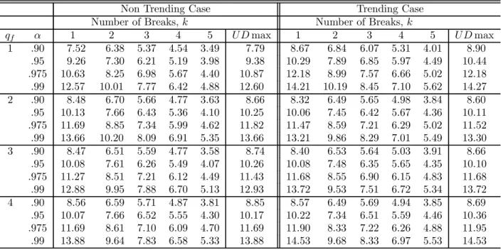
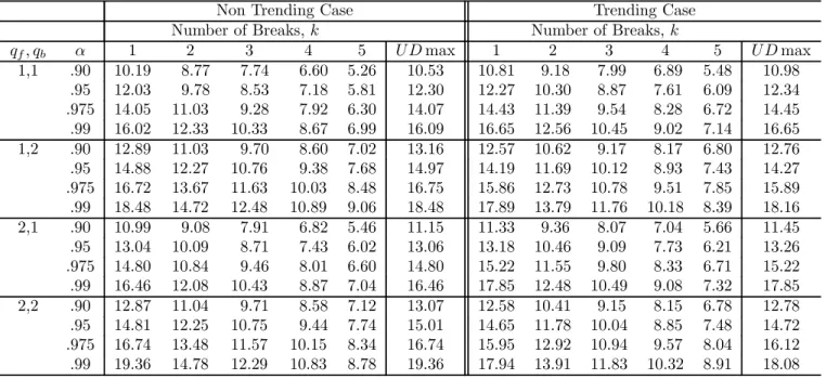
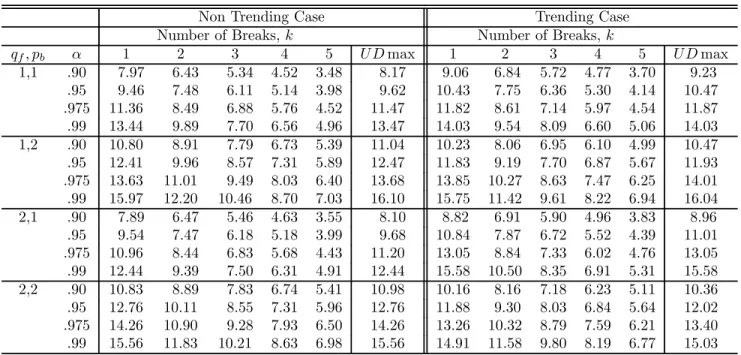
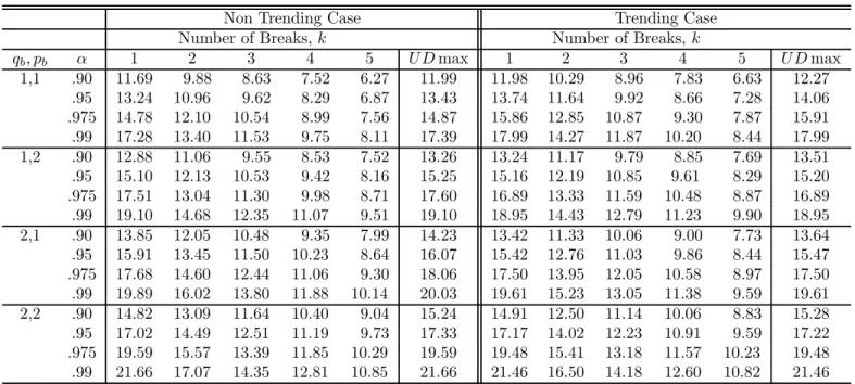
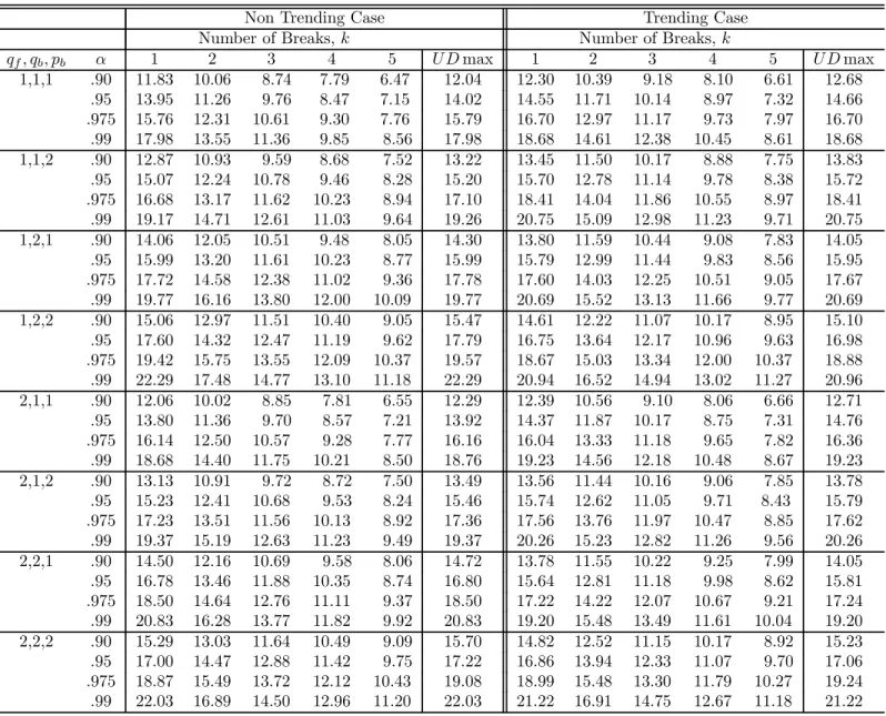
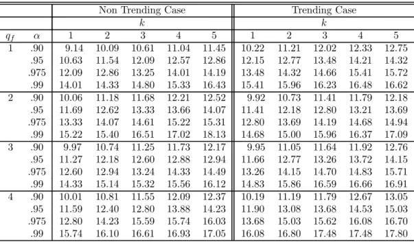
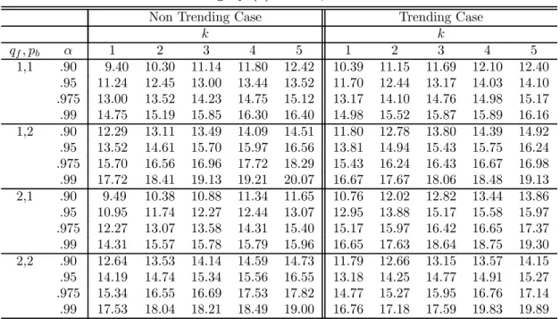
4.3 Asymptotic critical values
Since the asymptotic distributions are non-standard, critical values are obtained through simulations. These are provided for models with and without trends in regressors. We approximate the Wiener processes by partial sums of i.i.d. Normal random variables with
N = 500steps. The number of replications is 2000. For each replication, the supremum of
F(λ, k) with respect to (λ1, ..., λk) over the set Λk is obtained via a dynamic programming
algorithm (see Bai and Perron, 2003, for details). TheI(0) regressors are simulated as inde-pendent sequences ofi.i.d. N(0,1)random variables, and theI(1) regressors as independent random walks withi.i.d. N(0,1)errors (also independent of the I(0)regressors). The values of the trimming used are =.05, .10, .15, .20 and.25. Critical values are presented for up to9 breaks and4 regressors. The maximum number of breaks allowed is 8 when = 0.10,5 when = 0.15, 3 when = 0.20and 2 when = 0.25.For the UDmax test, M is set to 5or the maximum number of breaks possible. For models involving bothI(1)andI(0)variables, critical values are provided for all possible permutations up to2regressors of each type. For the limit distributions of the tests when the regressors contain trends and for the sequential tests, the critical values are tabulated for =.15, .20 and.25. Given the large number of results, we present critical values only for = 0.15in Tables 1 through 4. For other trimming values, tables of critical values are available on the authors’ website.
5 Extensions
We now extend the analysis of the previous Section to the cases where we can have either a) serially correlated errors in the cointegrating regression; b) endogenous regressors. We show that simple modifications yield tests with the same limit distributions as stated above.
5.1 Serially correlated errors: a modified sup-Wald test
With serially correlated errors, we use the following robust version of the scaled F test
FT∗(λ, k) = (T −(k+ 1)(qb+pb)−(qf +pf))
k γˆ
where Vˆ(ˆγ) is an estimate of the covariance matrix of ˆγ that is robust to serial correlation and heteroskedasticity; see Bai and Perron (1998) for details. Note that when testing for the stability of coefficients associated with I(1) variables, whether I(0) variables are included or not, we can simply apply the following transformation to the test in (3): F∗
T(λ;k) = ¡ ˆ σ2u/σˆ 2¢ FT(λ, k), where σˆ2u = T−1 PT t=1uˆ2t and ˆσ 2
is a consistent estimate of σ2. Since the break fractions are consistent even with serially correlated errors, we can first take the supremum of the originalF test to obtain the break points. The robust version of the test is then obtained by evaluatingF∗
T(λ;k)at these estimated break dates, i.e., the test considered
issupλ∈Λk FT∗(λ, k) =FT∗(ˆλ, k)whereλˆ = (ˆλ1, ...,λˆk)are the estimates of the break fractions
obtained by minimizing the global sum of squared residuals (2).
A problem with the Sup-Wald test is that with persistent errors, the size distortions can be substantial. The reason for this is the estimation of the long run variance using residuals under the alternative hypothesis. On the other hand, Vogelsang (1999) shows through simulation experiments that the estimation of the long run variance under the null hypothesis leads to the problem of non-monotonic power infinite samples. In a related paper, Crainiceanu and Vogelsang (2007) show that commonly used data dependent bandwidths for the estimation of the long run variance (based on the misspecified null model) are too large under the alternative hypothesis. This in turn leads to a decrease in power as the magnitude of the change increases. As a solution to this size-power trade-off, we use a new estimator of the long run variance constructed using a hybrid method that involves residuals computed under both the null and alternative hypotheses. In particular, the data dependent bandwidth is selected based on the residuals obtained under the alternative hypothesis. With this particular value of the bandwidth, the estimate is computed using residuals obtained under the null hypothesis of no structural change. Specifically, the proposed estimator is
ˆ σ2 =T−1 T P t=1e u2t + 2T−1 TP−1 j=1 w(j/ˆh) T P t=j+1e uteut−j (8)
where uet are the residuals obtained imposing the null hypothesis. The kernel functionw(·)
is the Quadratic Spectral and the estimate of the bandwidth is, following Andrews (1991), given byˆh= 1.3221(ˆa(2)T)1/5 where ˆa(2) = [4ˆρ2
/(1−ˆρ)4] andˆρ=PT
t=2uˆtuˆt−1/
PT
t=2uˆ2t−1, with uˆt the residuals from the model estimated under the alternative hypotheses. As we
later demonstrate, the sup-Wald test based on this estimator is able to bypass the problem of non-monotonic power while maintaining an exact size close to the nominal size. For more details on the merits of this approach, see Kejriwal (2008).
5.2 Endogenous I(1) regressors
Generally, the assumption of strict exogeneity is too restrictive and the test statistics devel-oped in the previous section are not robust to the problem of endogenous regressors. In this section, we use the linear leads and lags estimator (dynamic OLS) as proposed by Saikkonen (1991) and Stock and Watson (1993) and prove that the limiting distributions of the tests based on this estimator are the same as those obtained with the static regression under strict exogeneity. The modified regression is given by
yt= ˆci+zf t0 ˆδf +x0f tβˆf +zbt0 ˆδbi+x0btβˆbi+
T P
j=−T
∆zt0−jΠˆj + ˆvt∗ (9)
wherezt= (zf t0 , zbt0 )0. Note that the number of leads and lags of∆ztneed not be the same. We
specify the same value for simplicity. Alternatively, one can interpret T as the maximum
of the number of leads and lags. In order to prove our results, we need a few additional assumptions, which are the same that are required to show the consistency of the estimate of the cointegrating vector in the case of a model with no structural change.
Assumption A7: Let ζt = (ut, ufzt0, ubzt0)0 and ζzt = (u f0
zt, ubzt0)0. The spectral density matrix
fζζ(w) is bounded away from zero so that fζζ(w) ≥ αIn (n = qf +qb + 1) for w ∈ [0, π]
where α > 0. Also, the covariance function of ζt is absolutely summable, i.e., denoting
E(ζtζ0t+k) =Γ(k), we require thatP∞k=−∞||Γ(k)||<∞where|| · ||is the standard Euclidean norm. Denoting the fourth order cumulants of ζt by κijkl(m1, m2, m3), it is assumed that
P
m1 P
m2 P
m3|κijkl(m1, m2, m3)|<∞(where the summations run from−∞ to +∞).
Assumption A7 states the same conditions used by Saikkonen (1991) and allows to represent the error ut as follows: ut =
P∞
j=−∞ζ0zt−jΠj + vt, with
P∞
k=−∞||Πj|| < ∞
and where vt is a stationary process such that E(ζztvt+k) = 0, for all k, and fvv(w) =
fuu(w)−fuζz(w)fζzζz(w)
−1f
ζzu(w). The DGP under the null hypothesis is then
yt=c+zf t0 δf +x0f tβf + T P j=−T ∆zt0−jΠj +v∗t wherev∗
t =vt+P|j|>T ζz,t0 −jΠj ≡vt+et.The last requirements pertain to the possible rate
of increase of T asT increases. Following Kejriwal and Perron (2008a), these are given by:
Assumption A8: As T → ∞, T → ∞, 2T/T →0and T
P
|j|>T ||Πj||→0.
Note that A8 allows the use of information criteria such as the AIC or BIC. Since there can be serial correlation in the errors vt, we need to apply a correction for its presence.
estimates of the break fractions obtained by minimizing the global sum of squared residuals (2), and FD
T (λ, k) = T−1(SSRk/σˆ2v)FT(λ, k) with FT(λ, k) as defined in (3). We consider
an estimate σˆ2v based on a weighted sum of the sample autocovariances ofev∗
t, the residuals
obtained imposing the null, as defined by (8) withev∗
t instead ofuet(and using the unrestricted
residuals to obtain the bandwidth as discussed in the previous section). The relevant result is stated in the following Proposition.
Theorem 3 Under A1-A5 and A7-A8, for all testing problems the limit distributions of the test supλ∈ΛkFTD(λ, k), based on regression (9), are the same as those that apply to the test supλ∈ΛkFT(λ, k)under the added assumption of A6 and strict exogeneity withΩf1z =Ωb1z = 0.
6 Simulation experiments
We now present the results of simulation experiments that pertain to the size and power of the tests, including a comparison with the often used LM tests. Hansen’s (2000) method based on a “fixed regressors bootstrap” is also a possible avenue to provide valid large sample inference in some of the models considered. In theory, an advantage of his method is that it remains valid in the presence of changes in the marginal distributions of the regressors. We conducted extensive simulations and found that the Wald tests considered here are very robust to changes in the drift of the I(1) regressors and changes in the variance of the innovations driving them (as in the stationary case as reported by Hansen, 2000). Our asymptotic results provide tests with exact sizes close to nominal size, as we shall show.
6.1 The size of the tests
We start with the case where the DGP exhibits no structural change and hence analyze the size of the tests. The sample sizes considered are T = 120 and T = 240. The value of the trimming is set to .20. The maximum number of breaks (M) considered is 3. Depending on whether we correct for serial correlation and/or endogeneity, we have the following four specifications: (i) S_Corr=0, C_Corr=0: no correction for serial correlation or endogeneity; (ii) S_Corr=1, C_Corr=0: correction for serial correlation but not for endogeneity; (iii) S_Corr=0, C_Corr=1: correction for endogeneity but not for serial correlation; and (iv) S_Corr=1, C_Corr=1: correction for both endogeneity and serial correlation. To correct for serial correlation, we use the method discussed in Section 5.1. To correct for endogeneity, we use the dynamic OLS estimator, discussed in Section 5.2, with T = 2. The various DGPs
ηt ∼ i.i.d. N(0,1). The DGPs considered are, where et ∼ i.i.d. N(0,1) and Cov(ηt, et) =
0: DGP-1 (i.i.d. errors, exogenous regressor): ut = et; DGP-2 (AR(1) errors, exogenous
regressor):ut=ρut−1+et; DGP-3 (MA(1) errors, exogenous regressor):ut =et−θet−1; DGP-4 (i.i.d. errors, endogenous regressor): ut = 0.8ηt+et; DGP-5 (MA(1) errors, endogenous
regressor): ut= 0.5vt+ηt, vt=et−0.5et−1.
For each DGP, we consider the case where the regressors are{1, zt}and both the intercept
and the cointegrating coefficient are allowed to change across regimes. In all experiments,
1000 replications are used. All rejection frequencies are calculated at the nominal 5%level. Table 5 reports the empirical size, with T = 120 and 240 and ρ = θ = 0.5. Consider first the base case represented by DGP-1 where the regressor is strictly exogenous and the errors are i.i.d.. With S_Corr=0, C_Corr=0, the size is adequate for all the tests irrespective of the specification used. For DGP-2 with AR(1) errors, all tests show substantial distortions when we do not correct for serial correlation. However, using our proposed long run variance estimator, the size distortions are no longer present and the tests become somewhat conser-vative. With MA(1) errors (DGP-3), the tests have zero size when no correction for serial correlation is made. Again, the size is accurate once we use S_Corr=1. With endogeneity but no serial correlation (DGP-4), we see that all the tests have good size for S_Corr=0, C_Corr=1. Otherwise, size distortions up to 20% may occur. This shows that the correction for endogeneity based on the dynamic OLS estimator is quite effective. When both serial correlation and endogeneity are present (DGP-5), the tests have adequate size when we use S_Corr=1, C_Corr=1, although some mild distortions persist when testing for multiple breaks. WhenT = 240, for the DGP-5 and S_Corr=1, C_Corr=1, the rejection frequencies are reduced and even the multiple break tests become conservative.
We also considered the case where the regressors are {1, zt, xt}, with xt ∼i.i.d. N(1,1),
Cov(xt, ut) = Cov(xt, ηt) = 0, and the model allows the intercept and the cointegrating
coefficient to change across regimes but the coefficient of xt is held fixed. The results were
similar to those in Table 5. Hence, including an irrelevant I(0) regressor does not lead to any size inaccuracies over and above the case when they are not included.
6.2 A power comparison with the LM type tests
In this section, we analyze the power of the sup-Wald test and compare it with the sup, mean and exp-LM tests proposed in Hansen (1992b) and Hao (1996). Vogelsang (1999) and Crainiceanu and Vogelsang (2007) show that the power function of a wide variety of tests for a shift in the mean of a dynamic time series is non-monotonic with respect to the magnitude
of the break. One cause is the behavior of the estimate of the error variance in the presence of a shift in mean. In particular, theyfind that if the error variance is estimated under the null hypothesis, non-monotonic power can result. We show that the LM type tests suffer from the same problem in the cointegration setup and in certain cases, the power can go to zero as the magnitude of the break increases. Since the main issue pertains to the presence of serial correlation in the errors, we consider the case where the regressor is strictly exogenous and the trimming is set at = 0.15(we also performed simulation of the power of our tests with a DGP involving endogenous regressors and, actually, the power is enhanced relative to the exogenous regressor case). For the case with one break, the DGP is yt = zt+ut,
if t≤[T /2]andyt= (1 +δ)zt+ut, if t >[T /2], whereηt∼i.i.d. N(0,1), Cov(ut, ηt) = 0.
The sample size isT = 240. We consider DGP 2 (AR(1) errors) and 3 (MA(1) errors). The specification S_Corr=1, C_Corr=0 is used. We analyze the pure structural change model in which both the intercept and the cointegrating coefficient are allowed to change. The power functions are plotted in Figure 1. Considerfirst the case with AR(1) errors. The non-monotonicity of the power function of the LM tests is evident even at moderate values of δ. For very small values ofδ, the power of the mean LM test is slightly higher than the modified Wald test. This is due to the fact that the mean LM test is particularly suited to detect small changes (see Andrews and Ploberger, 1994). Surprisingly, however, the mean LM test performs better than the exp-LM test even for large changes. The sup-LM test is dominated by all tests irrespective of the sample size and the degree of persistence. With MA(1) errors, the picture is quite different. All tests have higher power compared to the autoregressive case although non-monotonicity is still evident for the LM tests. The performance of the LM tests is quite similar and no clear ranking emerges between them.
Next, we consider the case where the DGP involves 2 breaks and 3 regimes, specified by
yt=zt+ut, ift ≤[T /3],yt= (1 +δ)zt+utif [T /3]< t≤[2T /3]andyt=zt+utif [2T /3]<
t≤T, wherezt=zt−1+ηt,zt =zt−1+ηt,ηt∼i.i.d. N(0,1)andCov(ut, ηt) = 0. The power
functions are plotted in Figure 2. Consider first the case with AR(1) errors. Given that single break tests have difficulty in detecting such parameter changes, it is not surprising that all tests exhibit non-monotonic power. The modified sup-Wald test dominates all the LM tests regardless of the sample size and the extent of persistence. With MA(1) errors, again all tests display non-monotonicity although the power function of the modified Wald test is much higher than that of the LM tests. What is quite remarkable is the fact that the U Dmax test has, in all cases, a monotonic power function that is much higher than any of the other tests. This provides clear evidence to its usefulness.
Finally, it is useful to comment on what happens when the regression is spurious, i.e., there is no cointegration. Hansen (1992b) showed that the LM test designed to detect a martingale specification in the intercept, in the spirit of Nyblom’s (1989) test, can be viewed as a test for the null of cointegration against the alternative of no cointegration. Although the sup-Wald test is not specifically targeted for the alternative of random variation in the intercept, it still has power against spurious regressions (i.e., no cointegration). This means that it will also reject when no structural change is present and there is no cointegration (the errors are I(1)). However, we can use the following approach to determine if the data suggest structural changes in a cointegrating relationship or a spurious regression. Suppose that one is willing to put an upper bound M (say 5) on the number of breaks. Then if the system is cointegrated with less than M breaks, the sequential testing procedure can be used to consistently estimate the number of breaks. On the other hand, if the regression is spurious, the number of breaks selected will always (in large samples) be the maximum number of breaks allowed. Thus, selecting the maximum allowable number of breaks can be indicative of the presence ofI(1)errors. The same is true when information criteria are used to select the number of breaks. We verified via simulations that this is indeed the case.
7 Conclusion
We presented a comprehensive treatment of issues related to testing in cointegrated regression models with multiple structural changes. We analyzed models withI(1)variables only as well as models which incorporate bothI(0)andI(1) regressors. The breaks are allowed to occur either in the intercept, the cointegrating coefficients, the parameters of the I(0) regressors or any combination of these. Our simulation experiments show that the commonly used LM tests are plagued with the problem of non-monotonic power infinite samples. The sup-Wald test however is able to avoid such non-monotonicity while maintaining adequate size. Our asymptotic results allow us to devise a sequential procedure to select the number of breaks. Finally, we provide the asymptotic critical values of our tests for a wide range of models that are expected to be useful in practice. The simulation experiments demonstrate the favorable properties of our test and the proposed long run variance estimator. It is important to note that the idea of constructing the estimate of the long run variance using information under both the null and alternative hypothesis is quite general and is applicable even in regression models which do not involve structural change.
References
Andrews, D.W.K. (1991), “Heteroskedasticity and Autocorrelation Consistent Covariance Matrix Estimation,”Econometrica, 59, 817-858.
Andrews, D.W.K. (1993), “Tests for Parameter Instability and Structural Change with Un-known Change Point,” Econometrica, 61, 821-856.
Andrews, D.W.K., and Ploberger, W. (1994), “Optimal Tests when a Nuisance Parameter is present only under the Alternative,” Econometrica, 62, 1383-1414.
Bai, J. (1997), “Estimation of a Change Point in Multiple Regression Models,” Review of Economics and Statistics, 79, 551-63.
Bai, J., Lumsdaine, R.L., and Stock, J.H. (1998), “Testing for and Dating Breaks in Multi-variate Time Series,”Review of Economic Studies, 65, 395-432.
Bai, J., and Perron, P. (1998), “Estimating and Testing Linear Models with Multiple Struc-tural Changes,” Econometrica, 66, 47-78.
Bai, J., and Perron, P. (2003), “Computation and Analysis of Multiple Structural Change Models,”Journal of Applied Econometrics, 18, 1-22.
Bai, J., and Perron, P. (2006), “Multiple Structural Change Models: A Simulation Analysis,” inEconometric Theory and Practice: Frontiers of Analysis and Applied Research,D. Corbea, S. Durlauf and B. E. Hansen (eds.), Cambridge University Press, 212-237.
Carrion-i-Silvestre, J.L., and Sansó-i-Rosselló, A.S. (2006), “Testing the Null Hypothesis of Cointegration with Structural Breaks,” Oxford Bulletin of Economics and Statistics, 68, 623-646.
Crainiceanu, C.M., and Vogelsang, T.J. (2007), “Nonmonotonic Power for Tests of a Mean Shift in a Time Series,” forthcoming in Journal of Statistical Computation and Simulation. Davidson, J. (1994), Stochastic Limit Theory. Oxford University Press: Oxford.
Hansen, B.E. (1992a), “Efficient Estimation and Testing of Cointegrating Vectors in the presence of Deterministic Trends,”Journal Econometrics, 53, 87-121.
Hansen, B.E. (1992b), “Tests for Parameter Instability in Regressions with I(1) Processes,”
Journal of Business and Economic Statistics, 10, 321-335.
Hansen, B.E. (1992c), “Consistent Covariance Matrix Estimation for Dependent Heteroge-neous Processes,” Econometrica,60, 967-972.
Hansen, B.E. (2000), “Testing for Structural Change in Conditional Models,” Journal of Econometrics, 97, 93-115.
Hansen, P.R. (2003), “Structural Changes in the Cointegrated Vector Autoregressive Model,”
Hao, K. (1996), “Testing for Structural Change in Cointegrated Regression Models: Some Comparisons and Generalizations,”Econometric Reviews, 15, 401-429.
Kejriwal, M. (2008): “Tests for a Mean Shift with Good Size and Monotonic Power,” forth-coming in Economics Letters.
Kejriwal, M., and Perron, P. (2008a): “Data Dependent Rules for the Selection of the Number of Leads and Lags in the Dynamic OLS Cointegrating Regression,”Econometric Theory, 24, 1425-1441.
Kejriwal, M., and Perron, P. (2008b): “The Limit Distribution of the Estimates in Cointe-grated Regression Models with Multiple Structural Changes,”Journal of Econometrics,146, 59-73..
Kuo, B-S. (1998), “Test for Partial Parameter Instability in Regressions with I(1) Processes,”
Journal of Econometrics, 86, 337-368.
Ng, S., and Perron, P. (1997), “Estimation and Inference in Nearly Unbalanced and Nearly Cointegrated Systems,”Journal of Econometrics, 79, 53-81.
Nyblom, J. (1989), “Testing the Constancy of Parameters Over Time,”Journal of the Amer-ican Statistical Association, 84, 223-230.
Phillips, P.C.B., and Hansen, B.E. (1990), “Statistical Inference in Instrumental Variables Regression with I(1) Processes,” Review of Economic Studies,57, 99-125.
Perron, P. (2006), “Dealing with Structural Breaks,” inPalgrave Handbook of Econometrics, K. Patterson and T.C. Mills (eds.), Palgrave Macmillan, 278-352.
Perron, P., and Zhu, X. (2005), “Structural Breaks with Deterministic and Stochastic Trends,” Journal of Econometrics,129, 65-119.
Qu, Z. (2007), “Searching for Cointegration in a Dynamic System,” Econometrics Journal, 10, 580-604.
Qu, Z., and Perron, P. (2007), “Estimating and Testing Structural Changes in Multivariate Regressions,” Econometrica, 75, 459-502.
Quintos, C.E., and Phillips, P.C.B. (1993), “Parameter Constancy in Cointegrated Regres-sions,” Empirical Economics,18, 675-706.
Saikkonen, P. (1991), “Asymptotically Efficient Estimation of Cointegration Regressions,”
Econometric Theory, 7, 1-21.
Seo, B. (1998), “Tests for Structural Change in Cointegrated Systems,”Econometric Theory,
14, 222-259.
Stock, J.H., and Watson, M.W. (1993), “A Simple Estimator of Cointegrated Vectors in Higher Order Integrated Systems,”Econometrica,61, 783-820.
Vogelsang, T.J. (1999), “Sources of Nonmonotonic Power when Testing for a Shift in Mean of a Dynamic Time Series,”Journal of Econometrics, 88, 283-299.
Appendix
We use k.k to denote the Euclidean norm, i.e., kxk = (Ppi=1x2i)1/2 for x Rp. For a
matrix A, we use the vector-induced norm, i.e., kAk= supx6=0kAxk/kxk. We have kAk ≤
[tr(A0A)]1/2. Also, for a projection matrix P, kP Ak ≤ kAk. We use the notation Aei,j =
A(i,j) −A¯(i,j), where A(i,j) is the matrix of observations from regime i to regime j (both inclusive), i.e., A(i,j) = (aTi−1+1, ..., aTj)0 while A¯(i,j) is the matrix (conformable to Ai,j) of
means, i.e., A¯(i,j) = (¯ai,j, ...,a¯i,j)0 where a¯i,j = (Tj − Ti−1)−1P Tj
t=Ti−1+1at. Also, we use
A∗
(i,j) = A(i,j)−A¯
(i,j), where A¯(i,j) is the matrix (conformable to A
(i,j)) of sample averages, i.e., A¯(i,j) = (¯x, ...,x¯)0, where x¯=T−1PT
t=1xt. Let 1(i,j) be a (Tj−Ti−1)×1vector of ones. To ease notation, we will writeAe(i,i) as Aei, A∗(i,i) asA∗i, A¯(i,i) asA¯i, A¯(i,i) asA¯i and 1(i,j) as
1i,(W1, Wzf, Wzb, Wxf, Wxb)are independent Wiener processes with dimensions corresponding
to those of (B1, Bfz, Bzb, Bxf, Bxb). We also use the notation Wz = (Wzf0, Wzb0)0. We start with
a Lemma about the weak convergence of various sample moments whose proof is standard given the results in Qu and Perron (2007).
Lemma A.1 Under A1-A5, the following weak convergence results hold (for i= 1, ..., m+ 1): a) T−3/2P[T λi] t=1 zf t ⇒ Rλi 0 B f z, T−3/2 P[T λi] t=1 zbt ⇒ Rλi 0 B b z, T−1/2 P[T λi] t=1 u f xt ⇒ Bxf(λi), T−1/2P[T λi] t=1 u b xt ⇒ Bxb(λi), T−1/2 P[T λi] t=1 ut ⇒ B1(λi); b) T−2 P[T λi] t=1 zf tzf t0 ⇒ Rλi 0 B f zBzf0, T−2P[T λi] t=1 zbtzbt0 ⇒ Rλi 0 B b zBzb0; c)T−1 P[T λi] t=1 zf tut ⇒ Rλi 0 B f zdB1+λi(Σfz1+Λ f z1),T−1 P[T λi] t=1 zbtut ⇒ Rλi 0 B b zdB1+λi(Σbz1+Λbz1); d)T−1 P[T λi] t=1 zf tufxt0 ⇒ Rλi 0 B f zdBxf0+λi(Σf fzx+Λf fzx),T−1 P[T λi] t=1 zf tubxt0 ⇒ Rλi 0 B f zdBxb0+λi(Σf bzx+Λf bzx),T−1 P[T λi] t=1 zbtu f0 xt⇒ Rλi 0 B b zdBxf0+λi(Σbfzx+Λbfzx),T−1 P[T λi] t=1 zbtubxt0 ⇒ Rλi 0 B b zdBxb0+λi(Σbbzx+Λbbzx).
The next Lemma will also be useful in subsequent developments.
Lemma A.2 LetX¯i(Ti−Ti−1)×p) = (¯xi, ...,x¯i)
0,x¯ i = (Ti−Ti−1)−1 PTi t=Ti−1+1xtandμ i ((Ti−Ti−1)×p)= (μ, ..., μ)0. Then under A1-A4, we have for i = 1, ..., m + 1: (i) μi
− X¯i p −→ 0; (ii) T−1/2(X i −X¯i)0Ui = T−1/2(Xi −μi)0Ui +op(1); (iii) T−1(Xi −X¯i)0(Xi−X¯i) = T−1(Xi − μi)0(X i−μi) +op(1); (iv) T−3/2Zi0(Xi−X¯i) =T−3/2Zi0(Xi−μi) +op(1).
Proof of Lemma A.2: Part (i) follows trivially. To prove (ii), note thatT−1/2(X
i−X¯i)0Ui =
T−1/2(X
i−μi)0Ui+T−1/2(μi−X¯i)0Ui.We haveT−1/2(μi−X¯i)0Ui = (μ−x¯i)T−1/2PTt=iTi
−1+1ut=
op(1), using part (i). For (iii), note that
T−1(Xi−X¯i)0(Xi−X¯i) = T−1(Xi−μi)0(Xi−μi) +T−1(Xi−μi)0(μi−X¯i) +T−1(μi−X¯i)0(Xi−μi) +T−1(μi−X¯i)0(μi−X¯i) Now T−1(X i−μi)0(μi−X¯i) = T−1 PTi t=Ti−1+1(xt−μ)(μ−x¯i) 0 = −(λ i −λi−1)(μ−x¯i)(μ− ¯ xi)0 = op(1). Similarly, T−1(μi − X¯i)0(Xi − μi) = op(1). Finally, T−1(μi − X¯i)0(μi − ¯
Xi) = (λi −λi−1)(μ−x¯i)(μ−x¯i)0 = op(1). To prove (iv), note that T−3/2Zi0(μi −X¯i) =
T−3/2(PTi
Proof of Theorem 1: We only consider Cases (1) and (4). The details for the other cases can be found in the working paper version. We have
FT(λ, k) =
SSR0−SSRk
k(T −(k+ 1)(qb+pb)−qf −pf)−1SSRk
where SSR0 and SSRk are the sum of squared residuals under the null and alternative
hypotheses, respectively. In all cases, we havek(T−(k+1)(qb+pb)−qf−pf)−1SSRk p
→kσ2. Case 1: The regression under H1 isyt=ci+zbt0 δbi+ut and for SSR0 we have
SSR0 = (Y(1∗,k+1)−Zb∗(1,k+1)eδb)0(Y(1∗,k+1)−Zb∗(1,k+1)eδb) = (Zb∗(1,k+1)(δb−eδb) +U(1∗,k+1))0(Zb∗(1,k+1)(δb−eδb) +U(1∗,k+1)) = U(1∗0,k+1)U(1∗,k+1)−(Zb∗(10 ,k+1)U(1∗,k+1))0(Zb∗(10 ,k+1)Zb∗(1,k+1))− 1 (Zb∗(10 ,k+1)U(1∗,k+1)(A.1)) SSRk = kP+1 i=1 (Yei−Zebiˆδbi)0(Yei−Zebiˆδbi) = kP+1 i=1 (Zebi(δb−ˆδbi) +Uei)0(Zebi(δb−ˆδbi) +Uei) = kP+1 i=1{− (Zebi0 Uei)0(Zebi0 Zebi)−1(Zebi0 Uei) +Uei0Uei} Therefore, SSR0−SSRk ⇒ −σ2( R1 0W b(1,k+1) z dW1)0( R1 0W b(1,k+1) z Wzb(1,k+1)0)−1( R1 0W b(1,k+1) z dW1) +σ2 kP+1 i=1{ (Rλi λi−1W b(i,i) z dW1)0( Rλi λi−1W b(i,i) z W b(i,i)0 z )− 1(Rλi λi−1W b(i,i) z dW1)} +σ2 k P i=1 (λiW1(λi+1)−λi+1W1(λi))2 λi+1λi(λi+1−λi)
and the result stated follows. Case 4: The regression under the alternative hypothesis is
yt=ci+zf t0 δf +zbt0 δbi+ut. LetZ(1∗,k+1) = (Zf∗(1,k+1), Zb∗(1,k+1)) andeδ= (eδ 0 f,eδ 0 b)0. We have SSR0 = (Y(1∗,k+1)−Z(1∗,k+1)eδ)0(Y(1∗,k+1)−Z(1∗,k+1)eδ) = −(Z(1∗0,k+1)U(1∗,k+1))0(Z(1∗0,k+1)Z(1∗,k+1))−1(Z(1∗0,k+1)U(1∗,k+1)) +U(1∗0,k+1)U(1∗,k+1) SSRk = kP+1 i=1 (Yei−Zef iδˆf −Zebiˆδbi)0(Yei−Zef iδˆf −Zebiˆδbi) = kP+1 i=1 (Zef i(δf −ˆδf) +Zebi(δb−ˆδbi) +Uei)0(Zef i(δf −ˆδf) +Zebi(δb −ˆδbi) +Uei)
After considerable algebra, we can show that
SSRk = −( kP+1 i=1 e Z10iMbiUei)0( kP+1 i=1 e Z10iMbiZe1i)−1( kP+1 i=1 e Z10iMbiUei) − kP+1 i=1 (Zebi0 Uei)0(Zebi0 Zebi)−1(Zebi0 Uei) + kP+1 i=1 (Uei0Uei)
whereMbi =Ii−Zebi(Zebi0 Zebi)−1Zebi0 andIi the(Ti−Ti−1)×(Ti−Ti−1)identity matrix. Thus, SSR0−SSRk = −(Z(1∗0,k+1)U(1∗,k+1))0(Z(1∗0,k+1)Z(1∗,k+1))−1(Z(1∗0,k+1)U(1∗,k+1)) +( kP+1 i=1 e Zf i0 MbiUei)0( kP+1 i=1 e Zf i0 MbiZef i)−1( kP+1 i=1 e Zf i0 MbiUei) + kP+1 i=1 (Zebi0 Uei)0(Zebi0 Zebi)−1(Zebi0 Uei) +U(1∗0,k+1)U(1∗,k+1)− kP+1 i=1 (Uei0Uei) and, with Bf b z (r) = (Bzf(r)0,Bzb(r)0)0, SSR0−SSRk ⇒ −( R1 0B f b(1,k+1) z dB1)0( R1 0B f b(1,k+1) z B f b(1,k+1)0 z )−1( R1 0B f b(1,k+1) z dB1) +( kP+1 i=1 Rλi λi−1B M(i,i) z dB1)0( kP+1 i=1 Rλi λi−1B M(i,i) z B M(i,i)0 z )− 1(kP+1 i=1 Rλi λi−1B M(i,i) z dB1) + kP+1 i=1 (Rλi λi−1B b(i,i) z dB1)0( Rλi λi−1B b(i,i) z B b(i,i)0 z )− 1(Rλi λi−1B b(i,i) z dB1) + k P i=1 (λiB1(λi+1)−λi+1B1(λi))0(λiB1(λi+1)−λi+1B1(λi)) λi+1λi(λi+1−λi)
where BzM(i,i)(r) = Bzf(i,i)(r) −
Rλi λi−1B f(i,i) z Bzb(i,i)0( Rλi λi−1B b(i,i)
z Bzb(i,i)0)−1Bzb(i,i)(r). Note that
each element of BzM(i,i)(r) is the residual from the projection of the corresponding element
of Bzf(i,i)(r)onto the space spanned by {Bzjb(i,i)} qb
j=1 for a given realization of these stochastic processes. We also have BzM(i,i)(r) = (Ωf fzz)1/2WzM(i,i)(r), so that
kFT(λ, k) ⇒ −( R1 0W f b(1,k+1) z dW1)0( R1 0W f b(1,k+1) z Wzf b(1,k+1)0)−1( R1 0W f b(1,k+1) z dW1) +( kP+1 i=1 Rλi λi−1W M(i,i) z dW1)0( kP+1 i=1 Rλi λi−1W M(i,i) z W M(i,i)0 z )− 1(kP+1 i=1 Rλi λi−1W M(i,i) z dW1) + kP+1 i=1 (Rλi λi−1W b(i,i) z dW1)0( Rλi λi−1W b(i,i) z W b(i,i)0 z )− 1(Rλi λi−1W b(i,i) z dW1) + k P i=1 (λiW1(λi+1)−λi+1W1(λi))0(λiW1(λi+1)−λi+1W1(λi)) λi+1λi(λi+1−λi)
Proof of Theorem 2. We give the details only for cases 4 to 6. Case 4. The regression under H1 is yt =ci+zbt0 δbi+x0btβbi+ut. We have,
SSR0 = [Y(1∗,k+1)−Zb∗(1,k+1)eδb−Xb∗(1,k+1)eβb]0[Y(1∗,k+1)−Zb∗(1,k+1)eδb−Xb∗(1,k+1)eβb]
By Lemmas A.1 and A.2, T−3/2Z∗0
b(1,k+1)Xb∗(1,k+1) =op(1). Thus,
SSR0 = [Zb∗(1,k+1)(δb−eδb) +Xb∗(1,k+1)(βb−βeb) +U(1∗,k+1)]0×
[Zb∗(1,k+1)(δb−eδb) +Xb∗(1,k+1)(βb−βeb) +U(1∗,k+1)]
= (δb−eδb)0Zb∗(10 ,k+1)Zb∗(1,k+1)(δb−eδb) + 2(δb−eδb)0Zb∗(10 ,k+1)U(1∗,k+1)+U(1∗0,k+1)U(1∗,k+1)
= −(T−1U(1∗0,k+1)Zb∗(1,k+1))(T−2Zb∗(10 ,k+1)Zb∗(1,k+1))−1(T−1Zb∗(10 ,k+1)U(1∗,k+1)) −(T−1/2U(1∗0,k+1)Xb∗(1,k+1))(T−1Xb∗(10 ,k+1)Xb∗(1,k+1))−1(T−1/2Xb∗(10 ,k+1)U(1∗,k+1)) +U(1∗0,k+1)U(1∗,k+1)+op(1)
We have SSRk =
Pk+1
i=1[Yei−Xebiβˆbi−Zebiˆδbi]0[Yei −Xebiβˆbi−Zebiˆδbi]. Using Lemmas A.1-A.2,
T−3/2Ze0
biXebi =op(1) and underH0, Yei =Xebiβb+Zebiδb +Uei, so that
SSRk = kP+1 i=1 [Xebi(βb −βˆbi) +Zebi(δb−ˆδbi) +Uei]0[Xebi(βb −βˆbi) +Zebi(δb−ˆδbi) +Uei] = kP+1 i=1 [−(T−1Uei0Zebi)(T−2Zebi0 Zebi)−1(T−1Zebi0 Uei) −(T−1/2Uei0Xebi)(T−1Xebi0 Xebi)−1(T−1/2Xebi0 Uei) +Uei0Uei] +op(1) Therefore, kFT(λ, k) ⇒ −( R1 0W b(1,k+1) z dW1)0( R1 0W b(1,k+1) z W b(1,k+1)0 z )− 1(R1 0W b(1,k+1) z dW1) −Wxb∗(1)0Wxb∗(1)−W1(1)2 + kP+1 i=1 © (λi−λi−1)−1(W1(λi)−W1(λi−1))2 ª + kP+1 i=1 (λi −λi−1)−1(Wxb∗(λi)−Wxb∗(λi−1))0(Wxb∗(λi)−Wxb∗(λi−1) + kP+1 i=1 [(Rλi λi−1W b(i,i) z dW1)0( Rλi λi−1W b(i,i) z W b(i,i)0 z )− 1(Rλi λi−1W b(i,i) z dW1)]
which reduces to the expression stated in the Theorem. Case 5: The model under H1 is
yt=ci+zf t0 δf+x0f tβf+ut. We haveSSRk = Pk+1 i=1[Yei−Xef iβˆf−Zef iˆδf]0[Yei−Xef iβˆf−Zef iˆδf]. UnderH0, Yei =Xef iβf +Zef iδf +Uei, so that SSRk = kP+1 i=1 [Xef i(βf −βˆf) +Zef i(δf −ˆδf) +Uei]0[Xef i(βf −βˆf) +Zef i(δf −ˆδf) +Uei] Furthermore, T(ˆδf −δf) = (T−2Pki=1+1Zef i0 Zef i)−1(T−1Pki=1+1Zef i0 Uei) +op(1) and T1/2(ˆβf −βf) = (T−1 kP+1 i=1 e Xf i0 Xef i)−1(T−1/2 kP+1 i=1 e Xf i0 Uei) +op(1).
Hence, after some algebra,
SSRk = −(T−1 kP+1 i=1 e Ui0Zef i)(T−2 kP+1 i=1 e Zf i0 Zef i)−1(T−1 kP+1 i=1 e Zf i0 Uei) −(T−1/2 kP+1 i=1 e Ui0Xef i)(T−1 kP+1 i=1 e Xf i0 Xef i)−1(T−1/2 kP+1 i=1 e Xf i0 Uei) + kP+1 i=1 e Ui0Uei+op(1)
and kFT(λ, k) ⇒ −( R1 0W f(1,k+1) z dW1)0( R1 0W f(1,k+1) z Wzf(1,k+1)0)−1( R1 0W f(1,k+1) z dW1) +( kP+1 i=1 Rλi λi−1W f(i,i) z dW1)0( kP+1 i=1 Rλi λi−1W f(i,i) z W f(i,i)0 z )− 1(kP+1 i=1 Rλi λi−1W f(i,i) z dW1) + k P i=1 (λiW1(λi+1)−λi+1W1(λi)) 2 λi+1λi(λi+1−λi)
Case 6: The model under H1 is yt = ci + zbt0 δbi + x0f tβf +ut. In this case, SSRk =
Pk+1 i=1[Yei−Xef iβˆf −Zebiˆδbi]0[Yei−Xef iβˆf −Zebiˆδbi]. Under H0,Yei =Xef iβf +Zebiδb+Uei, so that SSRk= kP+1 i=1 [Xef i(βf −βˆf) +Zebi(δb−ˆδbi) +Uei]0[Xef i(βf −βˆf) +Zebi(δb−ˆδbi) +Uei]
We also have T(ˆδbi−δb) = (T−2Zebi0 Zebi)−1T−1Zebi0 Uei+op(1) and
T1/2(ˆβf −βf) = (T−1 kP+1 i=1 e Xf i0 Xef i)−1(T−1/2 kP+1 i=1 e Xf i0 Uei) +op(1). Hence, SSRk = − kP+1 i=1 (T−1Uei0Zebi)(T−2Zebi0 Zebi)−1(T−1Zebi0 Uei) −(T−1/2 kP+1 i=1 e Ui0Xef i0 )( kP+1 i=1 T−1Xef i0 Xef i)−1(T−1/2 kP+1 i=1 e Xf i0 Uei) + kP+1 i=1 e Ui0Uei so that kFT(λ, k) ⇒ kP+1 i=1 [−(Rλi+1 0 W b(1,i+1) z dW1)0( Rλi+1 0 W b(1,i+1) z Wzb(1,i+1)0)−1( Rλi+1 0 W b(1,i+1) z dW1) +(Rλi 0 W b(1,i) z dW1)0( Rλi 0 W b(1,i) z W b(1,i)0 z )− 1(Rλi 0 W b(1,i) z dW1) +(Rλi+1 λi W b(i+1,i+1) z dW1)0( Rλi+1 λi W b(i+!,i+1) z W b(i+1,i+1)0 z )− 1(Rλi+1 λi W b(i+1,i+1) z dW1)] + k P i=1 (λiW1(λi+1)−λi+1W1(λi)) 2 λi+1λi(λi+1−λi)
Proof of Theorem 3: We provide a proof for the testing problem (2) in Category (a), a pure structural change model with only I(1) regressors and a constant. The proofs for the other cases are very similar. We first let BeT = T−1/2
P[T r]
j=1eζj,where eζt = (vt, ubzt0)0. Under
the stated conditions, BeT ⇒ Be ≡ (B1.z, Bzb) as T → ∞, where B1b.z = B1 −Ωb1z(Ωbbzz)−1Bzb.
Note thatBb
1.z is independent ofBzb. Thus, Be denotes a vector Brownian motion with block
diagonal covariance matrix Ωe =diag((σb
1.z)2,Ωbbzz), where(σb1.z)2 =σ2−Ωb1z(Ωzzbb)−1Ωbz1. The relevant regression under the alternative hypothesis is
yt =ci+zbt0 ˆδbi+ T P
j=−T