AEM RESEARCH BULLETIN - 06-02
FINAL REPORT: MARCH 31, 2006
ECOSYSTEM VALUES AND SURFACE WATER PROTECTION: BASIC
RESEARCH ON THE CONTINGENT VALUATION METHOD
NATIONAL SCIENCE FOUNDATION GRANT SES - 0108667
Kent D. Messer1 Lara E. Platt1 Gregory L. Poe (P.I.)1
Daniel Rondeau
William D. Schulze (Co-P.I.)13 Christian A. Vossler
1. Cornell University, Department of Applied Economics and Management 2. University of Victoria, Department of Economics
Table of Contents
Page
i. Executive Summary
1. “Altruism in a Coercive Tax (Referendum) Setting: WTP and WTA for a Public Good,” Kent D. Messer, Gregory L. Poe,, Daniel Rondeau, William D. Schulze, and Christian A. Vossler.
81. “The Value of Private Risk Versus the Value of Public Risk: An Experimental Analysis,” Kent D. Messer, Gregory L. Poe, William D. Schulze.
126. “Certainty and Hypothetical Bias in Contingent Valuation Elicitation Methods,” Lara E. Platt, Kent D. Messer, and Gregory L. Poe.
Executive Summary
Project Background
In 1981, President Ronald Reagan issued Executive Order 12291. This order required that significant federal regulations undergo cost-benefit analysis before approval by the Office of Management and Budget. Every President since Ronald Reagan has continued to follow this policy. This research is primarily motivated by two important questions regarding the estimation of benefits associated with public goods for use in cost-benefit analysis.
First, in evaluating the benefits of providing public goods, many studies, especially those based on contingent valuation, have shown substantial evidence of altruistic values. Thus, individuals indicate that they are willing to pay not only for the benefits to themselves from a particular public good, but also are willing to pay for the benefits that others receive from the public good. Considerable debate has ensued concerning the legitimacy of including such altruistic values in cost-benefit analysis. This debate has focused on two forms of altruism, non paternalistic or pure altruism, and paternalistic or impure altruism. Pure altruism can be
characterized by the statement: “What I want for you is whatever makes you happy.”
Paternalistic altruism can be characterized by the statement: “I want for you whatever I think is good for you, whether you like it or not.” Pure altruism leads people to pay for others what others would pay for themselves and is generally viewed as leading to the double counting of benefits. In contrast, impure altruism motivates people to pay in addition to what others themselves would pay for a public good and is not viewed as double counting. Unfortunately, determining whether or not values for use in cost-benefit analysis incorporate altruism and what type of altruism is present is not easily accomplished. We address the empirical measurement of these forms of altruism in the first two papers of this report by developing and exploring the demand revelation characteristics of a new incentive compatible public goods elicitation mechanism we term the Random Price Voting Mechanism (RPVM) or the Voting Becker- DeGroot-Marshack (BDM) Mechanism.
The second issue we address is criterion validity in contingent valuation. In addition to providing a platform for examining the empirical components of altruism, the RPVM developed in this research offers a simulated market baseline for evaluating hypothetical bias in stated preference methods. The policy need for improved research in this area was highlighted by the Blue Ribbon Contingent Valuation Panel convened by National Oceanic and Atmospheric Administration (NOAA) in the wake of the Exxon Valdez oil spill and the consequent Oil Pollution Act of 1990.
Summary o f Paper 1
The first paper develops and tests a new public goods value elicitation mechanism, referred to as the Random Price Voting Mechanism (RPVM or the Voting Becker-DeGroot- Marshack (BDM) Mechanism), in a series of laboratory economics experiments. The hope is that this mechanism will allow exploration of the nature of altruistic values as well as provide a tool for calibrating hypothetical value questions obtained through surveys (contingent values). Note that many experiments have been utilized to calibrate hypothetical values for private goods since several demand-revealing private good mechanisms exist but few studies have been conducted for public goods. The reason for this discrepancy is that all of the demand-revealing mechanisms available for public goods are cumbersome or confusing at best (these include the Smith Auction
group interaction, and hence are not amenable to single-shot survey setting characterizing contingent valuation.
The experiments described use actual monetary payoffs and demonstrate that the RPVM is, in fact, demand revealing for both private and public goods. The data from these experiments further demonstrate that people do show non-paternalistic or pure altruism in voting on payoffs specified to each member of a voting group. In particular, voters with high payoffs from a program show concern for the cost/tax that voters with low payoffs will have to pay if the majority imposes a tax above the payoff for low payoff voters. Similarly, low payoff voters will vote for taxes above their payoffs so that high payoff voters will be better off. This behavior is consistent with pure altruism. Note that for public good settings in which voters all have identical payoffs, the voters tended to only vote yes if the payoff was greater than the cost. As such, for these baseline, homogeneous payoff cases, the mechanism is demand revealing.
Given that the RPVM is demand revealing and that it can reveal altruism in an induced value experimental setting, the second paper explores the possibility of paternalistic altruism in a risky environment. Such an extension is necessary because it is not possible to test for
paternalistic altruism using certain monetary payoffs. Rather, it is possible that people will have paternalistic preferences with respect to the financial risks that others face. The third paper uses the mechanism to calibrate hypothetical values collected using contingent valuation techniques.
Summary o f Paper 2
The purpose of this research is to develop a methodology to determine what types of altruism might be present in values obtained for cost-benefit analysis. The research utilizes the RPVM described in Paper 1. The methodology is tested for provision of group insurance to avoid a financial loss using laboratory economics experiments, more closely mimicking what is
referred to in the experimental economics and contingent valuation literature as home grown values (as opposed to an induced value setting utilized in the first paper). Yet, the methods used here can be employed either in the laboratory or field for other commodities more likely to yield paternalistic altruism. The type of altruism present in values is important since non-paternalistic or purely altruistic values should usually be excluded from cost-benefit analysis of the provision of public goods, but paternalistic altruism generally should be incorporated. The possibility of paternalistic altruism can be examined because participants in a voting group who prefer that others in their group do not accept a risk of loss, but do not care about their overall payoff, will always value insurance for their group (public good) above the value of insurance against the same risk for themselves alone (private good). Thus, in the case of homogeneous risks, where all members of a voting group face the same probability of loss and financial loss, paternalistic altruists will value group insurance more than insurance for themselves alone. In contrast, pure altruists will value group insurance the same as insurance for themselves alone.
No evidence for paternalistic altruism is found in this study. The pattern of values when different group members face different risks is, however, consistent with non-paternalistic or pure altruism as shown for certain payoffs in Paper 1. It should not be concluded from this single study that paternalistic altruism does not exist. Rather, the purpose of this study is to develop methods that can be used to determine whether paternalistic altruism exists in a particular setting. This method could be extended in future experiments that utilize other commodities to see if
reporting for public goods challenges the maintained assumption often asserted in valuation research that altruism leads to artificial inflation in reported benefits.
Summary o f Paper 3
This paper presents an analysis of hypothetical values for both private and public
insurance obtained under identical circumstances to those described for Paper 2. WTP values are again using the RPVM. The focus of this research is to test three separate contingent valuation elicitation methods for the degree of hypothetical bias in comparison with the actual values. Parallel hypothetical data is elicited for both private and public insurance policies using two forms of the Multiple Bounded Discrete Choice (MBDC) method described by Welsh and Poe (1998), and using the standard PC method (Rowe et al. 1996). In the standard PC format (Rowe et al. 1996), subjects circle a value corresponding with their decision from a table of values. A second sample received an alternative Dichotomous Choice Payment Card (DC-PC),
corresponding to that suggested in Boyle (2004) and employed by Bateman et al. (2005) amongst others. For the DC-PC, respondents indicate a vote of “Yes” or “No” to paying specified dollar amounts. As such, this elicitation method has similarities to the standard PC, but differs
fundamentally in that respondents are asked to register a decision for each dollar value (rather than simply circling one value from a table). A third sample faced a MBDC version requiring respondents to indicate a level of certainty of WTP for each of a series of values. Certainty response options in the MBDC format are “Definitely Yes” (DY), “Probably Yes” (PY), “Unsure” (UN), “Probably No” (PN), and “Definitely No” (DN). Past research (Vossler et al. 2004) indicates that the multiple bounded “Probably Yes” (PY) model best predicts actual behavior in contribution settings. To the best of our knowledge, such comparisons have not been provided for DC-PC and PC formats.
Results suggest in this case that the PC and MBDC-PY are significantly different in both the private and public goods settings. We also find that the PC and DC-PC estimates
significantly differ. However in all cases, the DC-PC and MBDC-PY estimates are nearly identical to the actual values. Nonparametric analysis shows that both the DC-PC elicitation format and the MBDC method, using a certainly level of Probably Yes, provide statistically similar estimates of WTP.
This finding indicates that calibration is possible to obtain accurate estimates of value using hypothetical questions in both private and public settings. A further implication of this research is that a simple DC-PC format may be preferred to the MBDC format in terms of predicting actual WTP, as well as being less cognitively taxing on the respondent. This
experimental economics laboratory research lays a foundation for extending such research to the field.
ALTRUISM IN A COERCIVE TAX (REFERENDUM) SETTING: WTP AND WTA FOR A PUBLIC GOOD
Kent D. Messer, Gregory L. Poe, and William D. Schulze Cornell University Daniel Rondeau University of Victoria Christian A. Vossler University of Tennessee September 15, 2005 Abstract
This report introduces a new “Voting-BDM” mechanism, which combines the Becker-DeGroot Marschak (BDM) mechanism for private goods with a majority voting rule. We use the Voting- BDM mechanism in an induced value framework to test the effect of pure altruism on the provision of public goods in coercive willingness-to-pay (WTP) and willingness-to-accept (WTA) settings for both gains and losses. Laboratory experiments indicate that with homogeneous induced values, the Voting-BDM mechanism is demand-revealing in both WTP and WTA settings. Consistent with our theoretical model, however, non-paternalistic altruism or fairness concerns appear to influence behavior when induced values are heterogeneous. With induced gains, better-off subjects under-report their WTP and WTA and worse-off subjects
over-report their WTP and WTA. The opposite holds true for induced losses.
The research in this paper was funded by National Science Foundation Grant (SES-0108667), USDA Regional Project W-1133, and the K. L. Robinson Endowment, Cornell University.
“How selfish soever man may be supposed, there are evidently some principles in his nature, which interest him in the fortune of others, and render their happiness necessary to him, though he derives nothing from it except the pleasure of seeing it.”
Adam Smith, Section I, Chapter. I,
The Theory o f Moral Sentiments
1. Introduction
The experimental economics literature has provided increasing evidence that other- regarding behavior is a significant factor in individual contributions and deviations from the dominant, Nash equilibrium strategy of no contributions in voluntary public goods settings (see for instance Andreoni, 1995; Palfrey and Prisbey, 1997; Goeree, Holt and Laury 1999; and Ferraro, Rondeau and Poe, 2003). This is problematic from the perspective of social decision making because it has long been recognized that, at the margin, the optimal provision of public goods should be based solely on selfish preferences (Bergstrom, 1982; Jones-Lee, 1991, 1992; Milgrom, 1993; Johansson, 1994). Hence, some types of other-regarding behavior, such as pure (or non-paternalistic) altruism and impure altruism (i.e., the warm glow of giving - Andreoni, 1990) should not be included in social benefit-cost analyses for small projects evaluated close to a social welfare optimum. One implication for the valuation of public goods is that individual, and therefore aggregate, willingness to pay (WTP) should be conditional on everybody else paying so as to remain at their initial level of utility (Johansson, 1994).
However, public projects are rarely, if ever, financed under such conditions: most
typically the funding for specific public projects imposes coercive costs that result in utility gains and losses. Moreover, projects evaluated tend to be discrete, and the initial allocation of public goods is inefficient. Under these conditions the extrapolation of Bergstrom’s result for marginal
analysis], determining whether a specific project can lead to a Pareto improvement” (Flores, 2002, p. 304; see also Johansson, 1993 and Johannesson, Johansson and O’Conor, 1996). Motives do matter.
Despite the fact that majority voting rules are increasingly used in ballot initiatives (referenda) to determine the provision of public programs that impose disproportionate costs and benefits on individuals, the effects of other-regarding behavior in involuntary, coercive settings are largely unexplored. To the extent that individuals exhibit other-regarding behavior, voting decisions are likely to be influenced by the perceived or actual impact on others (Deacon and Shapiro, 1975; Holmes, 1990). Understanding the motivation(s) and behavior of individuals who make personal choices affecting the public provision of public goods is therefore critical to benefit-cost analyses and the evaluation of the efficiency of referenda with coercive taxes.
To gain insights into individual behavior in coercive situations, we introduce a new public goods funding mechanism that combines the Becker-DeGroot-Marschak (BDM) (1964) mechanism for private goods with a majority voting rule. This we refer to as the Voting-BDM. For private goods, the BDM is theoretically incentive-compatible. Further, experimental evidence suggests that the BDM is a transparent mechanism with demand revealing properties (Boyce et al., 1992; Irwin et al., 1998). Laboratory experiments have further demonstrated the incentive compatibility and transparency of majority voting (see, for example, Plott and Levine
1978).
Whereas the BDM mechanism in a WTP setting has the subject purchase the good at a randomly determined cost whenever her maximum WTP is greater than or equal to the cost, the Voting-BDM implements the public good whenever a majority of subjects indicate a maximum
personal WTP, must pay this cost. In regards to a typical majority voting situation, note that the subject’s bid is an indication of the highest price at which they would still vote yes. In a WTA setting, subjects indicate their minimum WTA to forego the public good and if the majority of offers are less than or equal to the randomly selected compensation, then all subjects, regardless of their personal WTA, must accept this amount.
There are several reasons to study the Voting-BDM in an induced value, continuous response setting. First, contrary to actual, “real-world” majority voting settings whereby a
subject’s yes or no vote implies a WTP or WTA interval, the Voting-BDM elicits a welfare point estimate1. Second, the Voting-BDM is less complex than incentive compatible public goods funding mechanisms such as the Smith (1980) Auction and the Groves-Ledyard (1977) mechanism, with the single round and the transparent nature facilitating the examination of treatment effects. Third, providing only monetary incentives in a laboratory setting excludes the possible influence of paternalistic altruism, in which the donor’s utility is a function of particular consumption patterns of the beneficiary. Fourth, comparing Voting-BDM bids with induced values allows a direct test of warm glow. If no warm glow is evident in induced value monetary settings, any evidence of other-regarding behavior must be attributable to pure altruism.
The remainder of this report is organized as follows. The next section presents a
theoretical model and derives testable hypotheses of the effects of pure altruism on the behavior of subjects in a coercive tax setting. Section 3 discusses the experimental design, which includes various treatments under WTP and WTA settings for both induced gains and induced losses. Results appear in Sections 4 and 5. We conclude with a discussion of trends that are evident in
1 The submission of a bid is also more informative than a dichotomous “yes” or “no” response to a posted price which simply indicates that a subject’s value is above or below the specified cutoff. Hence the use of a continuous response function offers a more efficient means of investigating anomalous behavior in voting settings. In ongoing
these experiments and suggest areas for future research with the Voting-BDM mechanism. In concluding this report, we note that some of the suggestions made herein are being pursued in a NSF project that builds upon the present research (Schulze et al., 2004).
2._____A Theory of the Voting-BDM Mechanism and Testable Hypotheses
This section presents a theory of the Voting-BDM mechanism. For both clarity and brevity, we formulate this theory in the context of a “WTP-Gains” setting where individuals have a positive WTP for a public good. As we discuss below, the arguments in this setting are readily extendable to the other three possible welfare cases: willingness to pay to avoid a loss (WTP- Loss); willingness to accept compensation in lieu of a gain (WTA-Gain); and willingness to accept compensation to experience a loss (WTA-Loss). In the willingness-to-pay settings the reported values are referred to as “bids”. We refer to willingness-to-accept values as “offers”. Consider a situation where n individuals are asked to express the maximum amount of money they would be prepared to pay for a particular program. A program is heretofore defined as a known vector of values n = {nx,n
2
,..,nn) ,containing the payoff, ni , for individual i, and payoffs, TTj, that all other individuals in the voting group stand to receive if a majority of subjects express a WTP equal or above a per-person (or average) cost C. The ith individual’s revealed WTP amount or his bid is denoted Bt . The per person cost C is drawn from a uniform distribution in the interval [0,Cmax] . If a majority of bids are greater than or equal to C, individuali receives a monetary payoff Y + ni - C (which could be smaller than the subject’s initial endowment Y if ni < C).
(decreasing) in the gains (losses) of others. Thus, we posit that the total utility of individual i is
given by Ui = u Y + ni - C + ^ ( • (nJ - C)) I ,where a i > 0 is a parameter indicating the J ^
intensity with which individual i is affected by the gains and losses of others. This, in effect, adapts and extends the social welfare analysis of Charness and Rabin in three important dimensions. First, where Charness and Rabin are concerned with the case of two players, we allow for n players. Second, we do not restrict the analysis to linear utility functions. Third, and most importantly, since C is a stochastic variable, the game is one of incomplete information and the relevant framework of analysis will be expected utility with a Bayesian equilibrium concept. The term in the summation allows for the fact that subjects may have positive preferences for the benefits that others receive from the implementation of the program. The parameter a defines the extent to which the utility of individual i is affected by the potential gains (or losses) of others resulting from the implementation of the program. This formulation allows for
heterogeneity across subjects, including the purely self-interested case where a i = 0, Vi ^ j . Note further that a i is symmetric - implying that gains and losses are treated equally. The a i is also not recipient specific. Gains and losses of all j other individuals receive equal weight in i’s utility function.2
To compute the Bayesian Nash Equilibrium bid of individual i, it is useful to rank order the bids of all n-1 other individuals. Define Bm as the bid that ranks as the Integer ((n + 1)/2) th largest of those bids (for n=3 this is the smallest of the other two bids). It is also useful to define
Bk as the Round((n -1) / 2)th largest bid (for n=3, this identifies the largest of the other two bids). The interval [Bm , Bk ] defines the range over which a bid by voter i makes this individual have a
marginal influence over the outcome of the game (in a probabilistic sense, it makes him the median voter).
To see this, consider the expected utility of individual i, where B., are the bids from all other individuals in the voting group:
m | I EU, ( , B_ t)= | p(C )U Y + n - C + £ ( ■ ( n - C )) I ) C 0 V J B i I I + Jp ( c)U y +n - c + £ ( ■ ( *, - c ) ) Id c B m V ! * ' J B k C max
+ J p(C)U (Y)dC + J p(C)U (Y)dC
(1)
The first term denotes the expected utility conditional on the randomly drawn cost being below Bm, with p(C) representing the probability that a certain cost is drawn. In this case, i’s bid is completely irrelevant since there are a sufficient number of other voters who are willing to pay at least the drawn cost C to implement the program. The second and third terms represent the interval over which the bid of individual i will have a marginal effect. Here, Bt becomes the median bid. By increasing the bid amount individual i increases the probability that the program will be funded by increasing the range of costs that a plurality of voters is prepared to pay (second term), and decreasing the range over which the project is not implemented (third term). The last term is the interval of drawn costs for which, the program will not be implemented regardless of individual i’s bid, as too few individuals are prepared to pay the random cost and the project is not implemented.
Exploring the family of affine strategies, individual i conjectures that individuals m and k
Where yk and ym are positive constants, the exact value of which is defined by the equilibrium solution below. Substituting these expressions in Equation 1 and maximizing by choosing Bi
yields the first order condition:
P( B,) \ -U (Y)+ U Y + n - B ,+ L { a ,- (n, - B ,)) ) 0
J
This equation has a degenerate solution p (B,) = 0 (where Bi is set equal to the lower support of the cost distribution). Assuming concavity of the utility function, there is also an interior maximum whereby individual chooses his bid so as to equate the utility under the two alternative states of the world (the program is funded or it is not). This optimal bid is given by:
n + L a n j
B* =--- ^ --- (2)
1 + (n - 1)a
This optimal strategy has the same form as the prior of individual i regarding the bidding strategy of individuals k and m if one sets yt = 1/(1 + (n - 1)a ) . Therefore, a symmetric Bayesian Nash Equilibrium exists if all players adopt this linear strategy (including k and m of course). Note that an individual’s optimal bid only depends on his own parameters and knowledge of the payoff vector.
The individually rational bid prediction for the standard BDM is nested in (2). In the absence of other players, the summation term vanishes and n -1 = 0, yielding the well-known incentive compatibility result, B* = n . The model also predicts that if the payoffs are identical across subjects (nj=ni for all j), the optimal strategy is for the individual to bid an amount equal to his payoff(B* = n ) . In this case, the subjects sensibly recognize that if all individuals were to bid above the common value, the resulting increase in the probability that the program will be
funded is, in equilibrium, simply increasing the possibility that the program will be implemented at a cost above value, which will result in a net loss for all subjects, making bids above value irrational. Similar reasoning leads to the conclusion that bidding below the common value is also sub-optimal individually and collectively.
From (2), we can also predict how the optimal bid changes when payoffs are
heterogeneous across subjects. This is best accomplished by considering a departure from the equal payoff situation (n i = n j = n), for which we have already established that B* = n for all players. Note that from (2) any changes in the payoffs of others that leave the sum of payoffs unchanged (any change that preserves the mean of the payoffs of others) should have no impact on B*. Further inspection of (2) reveals that increasing (decreasing) the sum of other’s payoffs increases (decreases) the optimal bid. This yields the additional prediction that individual i will increase his bid from his value when, from a situation of equal payoffs, all payoffs but his are increased (his remains constant). Similarly, going from equal payoffs to a vector where all but i’s payoffs are decreased decreases the optimal bid of individual i from his payoff.
The theory is easily extendable to a “WTA-Gains” situation where individuals have positive value for the public good and are asked to express the minimum amount of money they
would be willing to accept to not implement the program. Let C now represent the randomly
determined compensation to forego the good and let Oi denote individual i’s offer or revealed WTA amount. If a majority of offers are less than or equal to C, the program is not implemented and each receives compensation such that monetary payoff is Y + C; otherwise, the program is implemented and payoff for individual i is equal to Y + ni . For this reinterpretation of model
parameters and trivial modification of the implementation rule, it can be shown that Equation 2 analogously determines optimal offer strategies for the WTA-Gains setting.3
A number of testable hypotheses emerge for the WTP-Gains and WTA-Gains settings. For the case where n=1, the Voting-BDM operates just like the traditional BDM mechanism. In this situation, the null hypothesis is for the individual to submit a bid or offer equal to their payoff:
HO : Bt (orO i) = n i if n=1. (3)
H f : B% (orOi)
When we move from the private or individual case to a homogenous public voting setting with n>1 and all individuals having equal payoffs, our theoretical framework predicts that an
individual bids (or offers) an amount equal to his value regardless of other-regarding preferences:
HO : Bt (or Oi) = n i if n>1 and ni = n j, Vj (4)
h 2A : B, (orO ,)
Note further that according to Hypothesis 1 and Hypothesis 2, a subject’s WTP (WTA) in a private good setting should be the same as a subject’s WTP (WTA) in a public good setting with homogeneous values, as both should equal the payoff amount. This finding would be strikingly different than behavior predicted and observed in other public good mechanisms, where subjects consistently report lower values in public good settings (Davis and Holt, 1993; Rondeau, Poe and Schulze, 2005). Because we do not formulate directional expectations, the null hypotheses are examined statistically using two sided significance tests.
In the general case where n>1 and values are heterogeneous, Equation 2 suggests that strategies are a function of the relationship between individual i’s payoff and the average payoff over all j individuals. If individual z’s payoff is equal to the average payoff of other individuals, he should submit a bid (offer) equal to his value regardless of other-regarding preferences. That is,
I n
H I : B} (or O, ) = n if n>1 and j — = x 1 (5)
n -1
H
3
: B, (orO ,)We refer to such an individual as a “mean-value” subject. Two other logical cases arise when individual i’s payoff is either greater than or less than the average of the voting group. We refer to individuals in the two cases as being “better-off’ and “worse-off’, respectively. For the purely self-interested individual (i.e., a, = 0), theory predicts that the individual bids (offers) his value in either case. In the presence of other-regarding preferences, however, our theoretical model predicts that the better-off subjects will bid (offer) below value and that worse-off subjects will bid (offer) above value. Given the assumptions of our model, behavioral predictions for better- off and worse-off subjects, under the null of no other-regarding preferences, are summarized below as hypotheses 4 and 5, respectively:
I v H 4
0
: Bi (or O,) = n i if n>1 and —---- < n i n -1 H 4 : B i (orO i) < n and (6)H / : Bi (orOi) > n
Since behavioral predictions for these two situations in the presence of other-regarding behavior are unidirectional, this implies one-tailed hypothesis tests.
When payoffs are negative (losses), subjects can be construed as expressing their maximum WTP to avoid losing this amount or minimum WTA to accept this loss. It is thus appropriate to compare the bid with the absolute value of the (negative) payoff via Equation 2. In absolute value terms, this leads to the same set of hypotheses for both gains and losses. Note however, that in absolute terms better-off subjects are those with lower than average payoffs and worse-off subjects are those with higher than average payoffs. To emphasize this distinction, we rewrite hypotheses 4 and 5 for the case of better-off and worse-off subjects, respectively, for losses: S K I H 0 : Bi 'o ' _P II if n>1 and J^L~ rn -1 > W (8) HA : Bi (orOi) > n and S K I H 0 : Bt (orO i) = n if n>1 and J ^ . 1 ^ 1 < n n -1 (9) HA : Bt (orOi) < n
where the alternative hypotheses imply one-tailed statistical tests. In the sections that follow we discuss an experimental design and the results of implementation of this design.
3.____ Experimental Design:
All experiments were conducted in the Laboratory for Experimental Economics and Decision-Making Research at Cornell University. One hundred and eighty-six subjects
volunteered for the experiments and were recruited from a variety of undergraduate economics courses. Each session consisted of either two WTP experiments: WTP-Gains and WTP-Losses (n=93) or two WTA experiments: WTA-Gains and WTA-Losses (n=93), thereby representing all four welfare settings.
All experiments use induced values (in absolute terms) of $2, $5 and $8, and each experiment consists of two parts. In the first part, subjects gain experience with the traditional BDM by engaging in 10 rounds with low financial incentives. The induced values vary randomly across rounds. In the second part, subjects go through one round each of nine different treatments with high financial incentives. Three treatments involve a group size of 1, which we refer to as the “private treatments”: (1) n=1, |n | = $2; (2) n=1, |n | = $5; and (3) n=1, |n | = $8. Three conditions involve a group size of 3 with homogeneous values, which we refer to as the
“homogeneous treatments”: (4) n=3, |n | = |n j = $2 V j; (5) n=3, |n | = |n; | = $5 V j; and (6) n=3,
|n | = |n | = $8 V j. The remaining three treatments involve a group size of 3 where the set of induced values for the group are $2, $5 and $8, and which we refer to as the “heterogeneous treatments”: (7) n=3, |n | = $2, |n | ^ \n\ V j; (8) n=3, |n | = $5, |n | ^ \n\ V j; and (9) n=3,
|n| = $8, |n | ^ V j. We provide subjects with complete information about the payoff amounts of the other subjects in Voting-BDM rounds.
Part B: WTP-Losses, nine high-incentive Voting-BDM rounds where the
treatment and cost which result in earnings is determined at the end of the experiment.
Part C: WTP-Gains, 10 low-incentive BDM rounds where the cost is determined and payoffs calculated at the end of each round.
Part D: WTP-Gains, nine high-incentive Voting-BDM rounds where the treatment and cost which result in earnings is determined at the end of the
experiment.
To control for potential order effects, the experiment order (gains or losses) varies across sessions. Further, Part B and Part D vary the order of the nine treatments across subjects. To prevent deterioration of other-regarding behavior that can occur in voluntary public good mechanisms (Davis and Holt 1993), subjects submit bids for the nine Voting-BDM treatments without feedback. At the end of the experiment, one of the nine Voting-BDM programs is implemented (and payoffs calculated) by having the subjects draw from a bag of marked poker chips. The exchange rate for the low-incentive BDM rounds is fifteen experimental dollars for one US dollar, while the exchange rate for the implemented Voting-BDM rounds is one experimental dollar for one US dollar. The experiment lasted approximately two hours and the average payoff was $35.
Subjects receive written instructions (Appendix A and B). As part of the verbal protocol, they are permitted to ask questions at the beginning of each part of the experiment. The
instructions use language parallel to that found in surveys for referendum voting settings (Carson et al., 2000). The WTP instructions direct each subject to vote whether to fund a program by submitting a bid that represents the “highest amount that you would pay and still vote for the program.” The WTA instructions direct each subject to vote whether to implement a program by
and still vote against the program.” Each subject was seated at an individual computer and an Excel spreadsheet was used to record bids and to calculate payoffs. Written voting sheets are collected after each round to determine the outcomes and to prevent subjects from revising their decisions.
Subjects are assigned to voting groups of varying size of either one or three. Obviously voting group of one corresponds to the private good situation where the single individual constitutes the median voter and the majority. For the groups of three, the administrators announced the groups and asked each group member to raise their hand so that they could be identified by other members of their group. This ensured that subjects were aware of who was in their voting group for all treatments. However, subjects did not know which of the other
members of the group received which payoff in the heterogeneous cases. As such, it is
reasonable to assume that the ai’s are not recipient specific. No communication was allowed and subjects in the same group size of three were not seated next to each other.
The cost amount (for WTP experiments) or compensation amount (for WTA
experiments) is determined by using a random numbers table with values from zero to nine. The first random number from the table represented the dollars amount, the second number the dimes amount, and the third number the pennies amount. For example, if the first random number was a four, the second was a nine, and the third a two, the determined cost (compensation) would have been $4.92. Consequently, the cost (compensation) is uniformly distributed between $0.00 and $9.99 with discrete intervals of $0.01.
A. WTP-Gains Experiment
In each round, subjects start with an initial balance of $10 and are assigned an induced value of $2, $5 or $8. For n=3 public treatments with heterogeneous values, an individual with an induced value of $2 is “worse-off’, a subject with $5 has “mean-value”, and an individual with a value of $8 is “better-off’. Subjects submit bids, ranging from zero to the entire initial balance, equal to the maximum amount for which they would still vote for the program. After the subjects submit their bids, the experiment administrator determines the random cost for the program. If the majority of the bids are greater than or equal to the randomly determined cost, then the program is funded. In this case, all of the subjects in the voting group receive their personal payoff amount in addition to the initial balance, but also have to pay the determined cost. If the majority of bids are less than the randomly determined cost, then the program is not funded. In this case, all of the subjects in the voting group neither receive their personal payoff amount nor pay the cost, and thus, the subjects receive only their initial balance.
B. WTA-Gains Experiment
In each round, subjects start with an initial balance of $5 and are assigned an induced value of $2, $5 or $8. This lower initial balance makes the expected earnings in the WTA setting equivalent to the WTP setting, thus allowing us to avoid possible income effects. For n=3 public treatments with heterogeneous values, an individual with an induced value of $2 is “worse-off’, a subject with $5 has “mean-value”, and an individual with a value of $8 is “better-off’. Subjects submit offers, ranging from zero to $10, which reflects their minimum WTA compensation to forego the public good. After the subjects submit their offers, the experiment administrator determines the randomly determined compensation for the program. If the majority of the offers
are less than or equal to the random compensation, then the program is not implemented and all group members receive the compensation in addition to their initial balance. If the majority of
offers are greater than the random compensation, the program is implemented and group
members receive their induced value in addition to their initial balance.
C. WTP-Losses Experiment
In each round, subjects start with an initial balance of $10 and are assigned an induced value of -$2, -$5 or -$8 such that the program is a public bad. For n=3 public treatments with heterogeneous values, an individual facing a loss of $2 is “better-off’, a subject facing a loss of $5 has “mean-value”, and an individual facing a loss of $8 is “worse-off’. Subjects submit bids, ranging from zero to the entire initial balance, equal to their maximum WTP to fund a program to forego the public bad. After subjects submit their bids, the experiment administrator
determines the random cost for the program. If the majority of bids are greater than or equal to
the determined cost, the program is funded, and all group members pay the cost from their initial balance of $10 but do not experience the public bad. If a majority of the bids is less than the random cost, the program is not funded. Consequently, all group members receive their initial balance plus the value of the public bad.
D. WTA-Losses Experiment
In each round, subjects start with an initial balance of $5 and are assigned an induced value of -$2, -$5 or -$8. For n=3 public treatments with heterogeneous values, an individual with an induced value of -$2 is “better-off’, a subject with -$5 has “mean-value”, and an individual
reflects their minimum WTA compensation to accept the public bad. After the subjects submit their offers, the experiment administrator determines the randomly determined compensation for the program. If the majority of the offers are less than or equal to the random compensation, then the program is not implemented and all group members receive the compensation, their induced value and their initial balance. If the majority of offers are greater than the random
compensation, the program is implemented and group members receive their initial balance only.
4. Results
A. Practice Rounds with Low Incentives
Similar to other studies using the BDM mechanism (Boyce et al., 1992; Irwin et al., 1998), the goal of the low-incentive rounds is to give subjects an opportunity to gain experience with the mechanism before introducing additional complexities to the decision environment. Repeated low-incentive BDM rounds provide subjects an opportunity to receive feedback on how their bids and offers affect payoffs. Over ten practice rounds, subjects bids/offers improved on average by 70% from $0.69 above induced value in the first round to only $0.21 above induced value in the tenth round (Figure 1). For the WTP practice rounds, the average bid decreased from $0.67 to $0.25 above induced value (an improvement of 63%). For the WTA practice rounds, the average bid decreased from $0.72 to $0.17 above induced value (an improvement of 76%). Overall, while learning was obviously taking place during practice rounds, by the last practice round subjects were submitting bids that are statistically indistinguishable from their induced values at the a=0.10 in all four welfare settings.
Figure 1. Low-Incentive Practice Rounds: Difference from Induced Value. — WTP-Gains WTP-Losses WTA-Gains WTA-Losses --- Linear (All)
1
2
3
4
5
6
7
8
9
10
Round B. Voting-BDMThe broad results from the four sets of voting BDM experiments can be most easily understood in the context of Figure 2 below. This figure provides aggregated willingness-to-pay and willingness-to-accept values for private and heterogeneous gains and losses as a function of induced values. Absolute values are used to enable pooling of losses and gains. The
willingness-to-pay and willingness-to-accept values for public homogenous voting settings are not provided in the figure as they are virtually indistinguishable from those for the private valuation settings4.
Figure 2: Aggregated Private and Heterogeneous Public Good Values Across Gains, Losses, WTP, WTA
-
45 Degree
• Private
—* — Heterogenous Voting
The close correspondence of private bid and offers with the 45 degree line equating the vertical and horizontal axis measures is evident in Figure 2. In contrast, average heterogeneous values intersect the 45 degree line from above. That is: at induced values of $2, the reported values exceed $2; at $5, induced and reported values are proximate; and at $8; reported values fall below induced values. These general trends are consistent with the other-regarding behavior hypotheses expressed above.
This general, intuitive presentation is reflected in the results of individual hypothesis tests. Our specific analyses of each of the voting-BDM hypotheses makes use of graphical presentations as well as formal econometric analyses. The graphical presentations provide the
basis for a more intuitive understanding of the nature of the shifts in valuation functions that occur across treatments. For the econometric analysis, we treat the set of decisions from each individual across high-incentive rounds as a panel data set and analyze the data using a two- factor fixed effects model. Indicator variables capture the differences across the (i=1,.. .,93) individuals, Di, as well as the (t=1,.. .,9) treatment conditions, It. The individual fixed effects capture the unobserved heterogeneity across individuals, such as differences in altruism. Specifically, for each of the four experiments we estimate the model:
Bit(or Oit) - n = C + Di + I t + (10)
where the dependent variable is the difference between individual i's bid and his induced value for treatment t; Z is an overall constant term; the Di and It are estimable fixed-effects parameters; and sit is a mean-zero random error term. Note that we do not have to worry about subject- specific autocorrelation here, as subjects do not receive any feedback until the end of the experiment (i.e., there are no learning effects). Also, no ordering effects are present since the sequence of treatments was randomized across individuals. The model is obtained by the inclusion of a full set of individual and treatment-specific indicator variables. The problem of perfect collinearity - the treatment and individual indicator variables both sum to one - is avoided by imposing the restrictions that the set of individual and treatment fixed effects independently sum to zero via a restricted least squares estimator.
We use the estimated models to test the hypothesized relationships between bids and induced values under the different treatment conditions and welfare settings as described in the Experimental Design section. The results of the hypothesis tests for the WTP-Gains, WTA- Gains, WTP-Losses, and WTP-Losses, respectively, are presented in Tables 1 through 4. The
terms) ($2, $5, and $8), different voting group sizes (one or three) and the distribution of induced values (homogeneous or heterogeneous). For brevity we omit the estimated equations in the text, providing the regression output in Appendix D. For all statistical tests below we employ a 5% significance level.
Hypothesis 1: Private Treatments. As demonstrated in Figure 3 and conjectured in the theoretical section, the distributions of bids and offers for the Voting-BDM with n=1 (which is equivalent to the conventional, private BDM) closely track induced values. The percent of optimal bids, defined as $4.99-$5.00 for the WTP treatments, ranged from 47% (WTP-Losses, $2) to 69% (WTP-Losses, $5). Similarly the range of optimal offers, defined as $5.00-$5.01 for the WTA treatments, ranged from 52% (WTA-Gains, $2) to 75% (WTA-Gains, $5). If each of these optimal ranges was increased to include induced value +/- 0.01 (e.g., $1.99-$2.01, $4.99-5.01, and $7.99-8.01), over 59% of the values would be deemed optimal in each of the treatments.
Table 1. WTP-Gains
Group Size = 1 Group Size = 3
Private P-value Homogeneous P-value Heterogeneous P-value
Low Value Mean $2.10 $2.06 $2.64 t
$2 Median $2.00 $2.00 $2.00
(Worst-off)
Difference from Induced Value $0.10 0.463 $0.06 0.694 $0.64 0.000
M iddle Value Mean $5.09 $5.11 $5.19
$5 Median $5.00 $5.00 $5.00
Difference from Induced Value $0.09 0.506 $0.11 0.427 $0.19 0.179
High Value Mean $8.11 $8.14 $7.78 t
$8 Median $8.00 $8.00 $8.00
(Best-off)
Difference from Induced Value $0.11 0.435 $0.14 0.314 -$0.22 0.061
n=93
Table 2. WTA-Gains
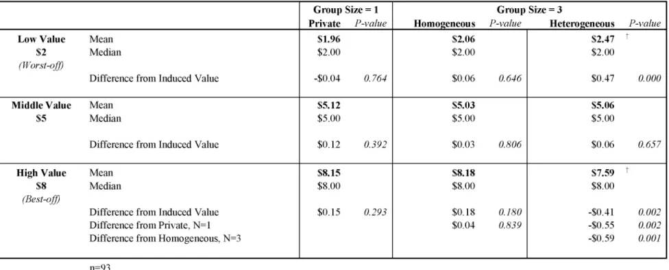
Group Size = 1 Group Size = 3
Private P-value Homogeneous P-value Heterogeneous P-value
Low Value Mean $1.96 $2.06 $2.47 t
$2 Median $2.00 $2.00 $2.00
(Worst-off)
Difference from Induced Value -$0.04 0.764 $0.06 0.646 $0.47 0.000
M iddle Value Mean $5.12 $5.03 $5.06
$5 Median $5.00 $5.00 $5.00
Difference from Induced Value $0.12 0.392 $0.03 0.806 $0.06 0.657
High Value Mean $8.15 $8.18 $7.59 t
$8 Median $8.00 $8.00 $8.00
(Best-off)
Difference from Induced Value $0.15 0.293 $0.18 0.180 -$0.41 0.002
Difference from Private, N=1 $0.04 0.839 -$0.55 0.002
Difference from Homogeneous, N=3 -$0.59 0.001
n=93
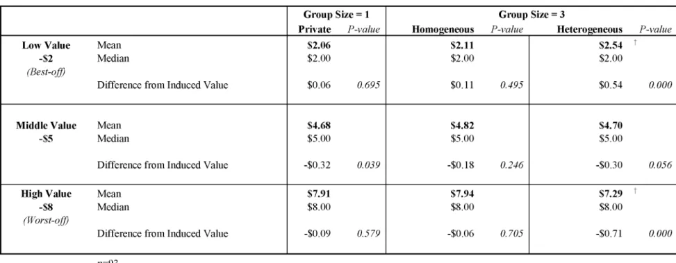
Table 3. WTP-Losses
Group Size = 1 Group Size = 3
Private P-value Homogeneous P-value Heterogeneous P-value
Low Value Mean $2.23 $2.14 $2.67 t
-$2 Median $2.00 $2.00 $2.00
(Best-off)
Difference from Induced Value $0.23 0.143 $0.14 0.368 $0.67 0.000
M iddle Value Mean $5.19 $5.00 $5.38
-$5 Median $5.00 $5.00 $5.00
Difference from Induced Value $0.19 0.241 $0.00 0.992 $0.38 0.017
High Value Mean $7.99 $7.80 $7.68 t
-$8 Median $8.00 $8.00 $8.00
(Worst-off
Difference from Induced Value -$0.01 0.928 -$0.20 0.201 -$0.32 0.020
n=93
Table 4. WTA-Losses
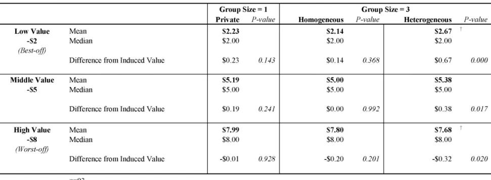
Group Size = 1 Group Size = 3
Private P-value Homogeneous P-value Heterogeneous P-value
Low Value Mean $2.06 $2.11 $2.54 t
-$2 Median $2.00 $2.00 $2.00
(Best-off)
Difference from Induced Value $0.06 0.695 $0.11 0.495 $0.54 0.000
M iddle Value Mean $4.68 $4.82 $4.70
-$5 Median $5.00 $5.00 $5.00
Difference from Induced Value -$0.32 0.039 -$0.18 0.246 -$0.30 0.056
High Value Mean $7.91 $7.94 $7.29 t
-$8 Median $8.00 $8.00 $8.00
(Worst-off)
Difference from Induced Value -$0.09 0.579 -$0.06 0.705 -$0.71 0.000
n=93
F re q u e n c y o f R e s p o n s e F re q u e n c y o f R e s p o n s e
Figure 3: Distribution of Private Bids and Offers for Each Induced Value (Absolute) in $0.25 Increments a. $2 -i j nnD IlLj-ip ^ F 1! 1 J 1! i'i *1 FT 1 1 i'i F 1 1 1*1 □ W T P -G a in □ W T P -L o s s □ W T A -G a in □ W T A -L o s s B id , O ffe r b. $5 ■ ■ i l l P1 i ° p P1 i i ■ ■ _ s S e T c c J -□ □ n □ W T P -G a in W T P -L o s s W T A -G a in W T A -L o s s
c. $8 & fr
s
3 I — n P n . . . p q P i p , n i i ,<*¥-
JNtJ
1—pV 1 □ W T P -G a in □ W T P - L o s s □ W T A -G a in □ W T A - L o s s B id , O ffe rSuch results are consistent with Irwin et. al (1998), who report that 62% and 67% of bids and offers, respectively, fell in the optimal range in a private BDM setting. These modal responses in the optimum range are reflected in measures of central tendency. In each of the private good cases, the median value equals the induced value (indeed, this result holds for all the treatments). Of the 12 private treatment scenarios (i.e., 3 treatments by 4 experiments), the null hypothesis is never rejected.
In all, although the presentation of the private BDM has changed by the addition of voting terminology in the instructions, the results from the voting-BDM, n=1
experiments are consistent with previous research demonstrating positive results for demand revelation characteristics of willingness-to-pay and willingness-to-accept values in private BDMs.
Hypothesis 2: Homogeneous Treatments. As might be expected from the aggregated mean WTP bids across treatments reported in Footnote 6 and presented in Figure 2, homogeneous WTP and WTA distributions closely correspond with the respective distributions of private bids and offers as well as of induced values. As a representative example, we provide the private and homogenous distributions for WTP-Gains for induced values of $2, $5 and $8 in Figure 4. The correspondence between the private distributions for other treatment/induced values can be gleaned from Figures 5-9. These graphical impressions are reflected in the econometric analysis. In public treatments with homogeneous values, average voting-BDM bids or options are not statistically different from induced values, such that we fail to reject Hypothesis 2 in all treatments in all experiments. These results are summarized in Tables 1 - 4 and porivde in detail in Appendix D.
Figure 4: Private and Homogenous WTP-Gains Bids a. $2 £ O '< P 3 □ ro 3 E 3
b. $5 c o 4! 3 J2 ■c Q n 3 O 90 80 70 6 0 50 4 0 30 2 0 10 100 » — ■ 4 I ---^---. - A ^ 4 ---aa...* ---$ 2 $ 4 $ 6 B id A m o u n t $ 8 $ 1 0 0 $ $ 5 - P riv a te $ 5 -H o m o g e n e o u s c. $8 •>? 0s c 0 43! 12 ■c ts
s
1 ra 3 E 3 W T P -G A IN S $8 C u m u la tiv e D is trib u tio n s100 90 80 70 6 0 50 4 0 30 2 0 10 0 $■ .1 .7 . . A - * - -•****■* _ +_________- - ' $ 2 $ 4 $ 6 $ 8 $ 1 0 $ 8 - P riv a te $ 8 -H o m o g e n e o u s
The statistical similarity between induced and reported values in the homogeneous voting setting contrasts with other popular single-shot public goods mechanisms, such as the Voluntary Contributions Mechanism or Provision Point Mechanism, where subjects with homogeneous values systematically bid below value for induced gains in the range of values studied here. Note that if warm-glow were a significant factor here then we would expect significant deviations from induced value, namely positive deviations in the WTP experiments (Rondeau, Poe and Schulze, 2005). Since this is clearly not the case, it appears that impure altruism/warm glow does not contaminate the results from the public heterogeneous treatments. Hence, any differences from induced values in the
heterogeneous settings may be attributable to pure altruism in this study. We turn to this issue now.
Hypothesis 3: Heterogeneous Treatments - Mean-value Subjects. The behavior of mean- value subjects in public heterogeneous treatments does not follow a consistent pattern relative to the private and public homogenous distributions, and may vary depending upon the framing of the situation. This lack of pattern is evident in Figure 5, which compares the private, public homogenous and public heterogeneous distributions of bids and offers for the $5 induced values in each of the four treatments. Indeterminacy in directional effects carries over to the econometric estimates, with some of the mean differences between reported and induced values being positive and others being negative. Nevertheless, although there appear to be some movement in distributions,
Hence, Hypothesis 3 cannot be rejected, lending some tentative support to the conclusion that gains and losses across other individuals are judged symmetrically.
Figure 5: Private, Public Homogeneous, and Public Heterogeneous Bid Distributions: Mean Value Subjects $5, -$5
C u m u la ti v e D is tr ib u ti o n s (% ) b, WTP-Losses c. WTA-Gains
d. WTA-Losses
Hypothesis 4: Heterogeneous Treatments - Better-Off Subjects, Gains. In contrast to the mean-value subjects, there is a notable directional effect of heterogeneity on the
distribution of bid and offer values (Figure 6). For gains, the distribution functions of bid values for the better off subjects ($8) shifts leftwards, with notable movement in the lower part of the distribution, suggesting that some subjects demonstrate other-regarding behavior by reducing their bids or offers (votes) downward. In these treatments, subjects submit bids or offers that are an average of $0.22 below (WTP-Gains, Table 1) and $0.41 below (WTA-Gains, Table 2) their induced value, respectively. While this altruism effect is significant in the WTA setting, the p value in the WTP treatment is 0.061 and thus not significant at the 5% level used in this analysis. For statistical comparisons associated
with hypotheses 4 - 7, this marginal rejection is the only failure to reject the null hypotheses using a 5% significance level.
Hypothesis 5: Heterogeneous Treatments - Worse-Off Subjects, Gains. In contrast, as predicted by our theoretical framework, the bids and offers for worse-off subjects submit increase in heterogeneous settings, with notable shifts in the upper parts of the
distributions (see Figure 7). On average, subjects report bids of $0.64 above their induced value in WTP-Gains (Table 1). In WTA-Gains, the worse-off subjects report offers that are statistically higher then their induced value by an average of $0.47 (Table 2). In both settings, the differences are significant, thereby rejecting the null hypothesis.
C u m u la ti v e D is tr ib u ti o n s (% ) C u m n lu a ti v e D is tr ib u ti o n s ( % )
Figure 6: Heterogeneous Treatments, Bid and Offer Distributions Better Off Subjects - Gains
a. WTP-Gains - $8
B id A m o u n t
a. WTP Gains - $2
Figure 7: Heterogeneous Treatments, Bid and Offer Distributions Worse-Off Subjects - Gains
B id A m o u n t
Hypothesis 6: Heterogeneous Treatments - Better-Off Subjects, Losses. In heterogeneous treatments with induced losses, behavior from the better-off subjects shows evidence of significant other-regarding behavior. As discussed earlier, with induced losses the better- off subjects in the public heterogeneous treatments inur induced losses of -$2.00.
Therefore, our economic-theoretic construct predicts that best-off subjects will over report their WTP and WTA. Indeed, best-off subjects submitted average bids of $2.67 and $2.54 (Table 3 and Table 4, respectively), which are significantly above their induced value, thereby rejecting the null hypothesis. These average results are reflected in the distributional shifts presented in Figure 8.
Hypothesis 7: Heterogeneous Treatments - Worse-Off Subjects, Losses. With losses, the worst-off subjects had induced losses of -$8.00 and our theoretical framework predicts that they would under-report their WTP and WTA. Consistent with this prediction, the worse-off subjects submitted bids that were $0.32 below the induced value in WTP- Losses and $0.71 below in WTA-Losses (Table 3 and Table 4, respectively). These distributional shifts are significant, and, as depicted in Figure 9, mirror those of the previously discussed with the greatest shifts occurring a the lower end of the distribution.
c im ij a ti v e Q s tr ib u ti c n s (% ) C u m u la ti v e D is tr ib u ti o n s (% )
Figure 8: Heterogeneous Treatments, Bid and Offer Distributions Better-Off Subjects - Losses
a. WTP Losses - $2
a. WTP-Losses - $8
Figure 8: Heterogeneous Treatments, Bid and Offer Distributions Worse-Off Subjects - Losses
B id A m o u n t b. WTA-Losses - $8 1 0 0 -|
______________________________________ J
- - * - - $ 8 - P riv a te $ 8 -H o m o g e n e o u s 80 r 6 0 'C 50S
4 01
H e te ro g e n e o u s 2 0 ^______ / 10 0 ^ ^ _____w m ^M _ $ - $ 2 $ 4 $ 6 $ 8 $ 1 05. Conclusion
The empirical evidence presented in this report demonstrates that the public good version of the incentive compatible BDM mechanism, when combined with voting in a coercive tax setting, is demand revealing. This is demonstrated by the failure to reject the null hypotheses that bids and offers equal induced values in private and homogeneous settings. Because there is no overbidding in the homogeneous settings, warm glow or impure altruism does not appear to carry over to this mechanism. In addition, the use of monetary incentives excludes the possibility of paternalistic altruism and both WTP and WTA approximate induced values (and hence approximate each other). However, concerns about equity arise with this mechanism. That is, subjects with high induced gains tend to understate their WTP and WTA in a public good coercive tax setting with a heterogeneous distribution of induced values. This pattern is mirrored in the induced loss treatments where the subjects with low induced losses demonstrate other-regarding concern by overstating their WTP.
The results of these experiments indicate that other-regarding behavior in a coercive tax setting is quite different that found in voluntary contribution settings. The experiments presented in the paper represent a potential starting point from which these issues can be examined further, and assumptions in our theoretical framework can be relaxed. Promising extensions of this include changes in voting group size when values are heterogeneously distributed and changes in the distributions of the heterogeneous treatments. Given our positive results using induced values, we maintain that this
revealing characteristics of this mechanism offers a means for exploring various behavioral anomalies in the context of public settings.
References
Andreoni, J. 1990. Impure Altruism and Donations to Public Goods: A Theory of Warm
Glow Giving. The Economic Journal 100(401): 464-477.
Andreoni, J. 1995. Cooperation in Public Goods Experiments: Kindness or Confusion?
American Economic Review 85: 891-904.
Becker, G.M., M.H. DeGroot, and J. Marschak. 1964. Measuring Utility by a Single Response Sequential Method. Behavioral Science 9: 226-32.
Bergstrom, T. C., 1982. “When is a Man’s Life Worth More then His Human Capital?” in Jones-Lee, M. W. (ed.), The Value of Life and Safety, North-Holland,
Amsterdam.
Boyce, R.R., T.C. Brown, G.H. McClelland, W.D. Schulze, and G.L. Peterson. 1992. An
Experimental Examination of Intrinsic Environmental Values. American
Economic Review 82(5): 1366-1372.
Carson, R.T., T. Groves, and M.J. Machina. 2000. Incentive and Informational Properties
of Preference Questions. Unpublished Manuscript (February).
Charness, G. and M. Rabin. 2002. Understanding Social Preferences with Simple Tests.
The Quarterly Journal o f Economics. 117(3): 817-869.
Davis, D.D. and C.A. Holt. 1993. Experimental Economics. Princeton, New Jersey: Princeton University Press.
Deacon, R.T., and P. Shapiro. 1975. “Private Preference for Collective Goods Revealed
through Voting on Referenda,” American Economic Review 65: 943-955.
Ferarro, P. J., D. Rondeau, and G. L Poe. 2003. Detecting Other-Regarding Behavior with Virtual Players. Journal o f Economic Behavior and Organization 51(1): 99
109.
Flores, N. E., 2002. Non-Paternalistic Altruism and Welfare Economics, Journal o f
Public Economics, 83:293-305.
Goeree, J. K., C. A. Holt, and S. K. Laury. 1999. Altruism and Noisy Behavior in One- Shot Public Goods Experiments. Manuscript, Department of Economics,
Holmes, Thomas P. (1990). “Self-Interest, Altruism, and Health Risk Reduction: An
Economic Analysis of Voting Behavior,” Land Economics 66(2): 140-149.
Irwin, J.R., G.H. McClelland, M. McKee, W.D. Schulze, and NE. Norden. 1998. Payoff
Dominance vs. Cognitive Transparency in Decision Marking. Economic Inquiry
36(2): 272-285.
Johannesson, M., P-O. Johansson, and R.M. O’Conor. 1996. The Value of Private Safety Versus the Value of Public Safety. Journal o f Risk and Uncertainty 13: 263-275. Johansson, P-O, 1993. Cost Benefit Analysis of Environmental Change, Cambridge
University Press, Cambridge, UK.
Johansson, P-O, 1994. Altruism and the Value of Statistical Life: Empirical Implications,
Journal o f Health Economics, 13:111-118.
Jones-Lee, M. W., 1991. Altruism and the Value of Other People’s Safety, Journal o f Risk and Uncertainty, 4: 213-219.
Jones-Lee, M. W., 1992. Paternalistic Altruism and the Value of Statistical Life, The Economic Journal 102: 80-90.
Milgrom, P. R., 1993. Is Sympathy an Economic Value? Philosophy, Economics and the Contingent Valuation Method, in Hausman, J. A. (ed.), Contingent Valuation: A Critical Assessment. Amsterdam: North-Holland.
Palfrey, T. P. and J. E. Prisbey. 1997. Anomalous Behavior in Public Goods
Experiments: How Much and Why? American Economic Review 87: 829-846.
Plott, C.R. and M. Levine. 1978. A Model of Agenda Influence on Committee Decisions.
American Economic Review (68): 147-160.
Poe, G.L., J.E. Clark, D. Rondeau and W.D. Schulze. 2002. Provision Point Mechanism
and Field Validity Tests of Contingent Valuation. Environmental and Resource
Economics 23: 105-13.
Rondeau, D., G.L. Poe, and W.D. Schulze. 2005. VCM or PPM? A Comparison of the
Performance of Two Voluntary Public Goods Mechanisms. Journal o f Public
Economics. 89:1581-1592.
Rondeau, D., W.D. Schulze, and G. L. Poe. 1999. Voluntary Revelation of the Demand
for Public Goods Using a Provision Point Mechanism. Journal o f Public
Schulze, W.D., H.M. Kaiser, K.D. Messer, and G.L. Poe. 2004. An Experimental Economics Examination of Behavioral Anomalies, Group Decision Making, and the Provision of Public Goods, NSF-Grant SES-0418450.
Smith, A., 2000. The Theory of Moral Sentiments, Prometheus Book, Amherst, NY Smith, V.L. 1979. Incentive Compatible Experimental Processes for the Provision of
Public Goods, in V.L. Smith, ed., Research in Experimental Economics, vol. 1. Greenwich, Conn.: JAI Press.