Lifted Variational Inference

Lifted Relational Variational Inferences

Jaesik Choi [email protected]

Eyal Amir [email protected]

Computer Science Department,

University of Illinois at Urbana-Champaign, Urbana, IL 61801 USA

Abstract

We present a lifted inference algorithm for relational hybrid graphical models. Hy-brid graphical models with continuous and discrete variables naturally represent many real-world applications in robotics, financial market predictions, and weather analysis. Inference with such large models is challenging because relational structures deteriorate rapidly with current inference procedures. The main contribution of this paper is a rela-tional variarela-tional-inference lemma that enables factoring density functions into a mixture of independent identically distributed multi-valued Bernoulli trials. This lemma enables a relational factoring step that takes hybrid ground potentials and finds a close to optimal lifted relational model for the joint density. This step is then used for efficient inference without referring to ground random variables. The new method allows us to build var-ious efficient inference algorithms. As an example, we provide a lifted Markov Chain Monte Carlo (MCMC) algorithm that requires fewer samples and generates each sam-ple faster than possible before. We provide an error analysis of the variational method when applying to relational models. Our approach is applicable to general large relational models.

1. Introduction

Many real world systems can be described using continuous and discrete variables with relations among them. Such examples include measurements in environmental-sensors networks, localizations in robotics, and economic forecasting in finance. In large such

systems, efficient and precise inference is essential. As an example from environmental

science, an inference algorithm can predict a posterior of unobserved water levels and

contamination levels at different locations, and making such inference precisely is critical

to decision makers.

Relational Probabilistic Languages (RPLs) [14, 16, 10, 17, 7, 19, 13, 11, 2] describe prob-ability distributions at a relational level with the purpose of capturing structure of larger models. These compact representations can facilitate the construction and learning of probabilistic models for large systems. A key challenge of inference procedures with RPLs is that they often result in density functions involving many random variables.

Recent advances (e.g. [7, 13, 11]) presented approaches to inference that (among others)

group equivalent models into a histogram representation which includes an order ofnk−1

entries (instead of performing kn−1 operations on traditional ground models)). Further,

approximate lifted inference algorithms (e.g. [20, 1]) extended this approach and showed how to solve such inference problems with belief propagation and sampling (e.g. [21]).

….

1 2

( ( ),

( ),

,

( ))

X

X a

X a

X a

n

φ

L

….

X

Φ

|

) |

)

))

( (

( (

X i X X I i

P X

X

I

a

a

φ

=

|

(

)

_i

(

( ))

X X X I i I_X

Φ

I

∏

φ

_X

X a

∫

X

I

X

φ

1

( )

X a

X a

( )

₂

X a

(

_n

)

X a

( )

₁

X a

( )

₂

X a

(

_n

)

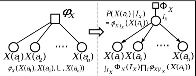
Figure 1: Illustration of a way to transform a potential with n exchangeable random

variables (X(a1),· · ·,X(an)) into a variational model with a latent variableIX. The variational

form (the right hand side) allows a compact representation with fewer parameters.

Unfortunately, these principles are not applicable to continuous or hybrid models, where

kis large or infinite.

In this paper, we present an approach to relational lifted inference in Hybrid models. It applies a relational variational-inference lemma that we prove and that enables factor-ing density functions into a mixture of independent identically distributed multi-valued Bernoulli trials. This lemma enables a relational factoring step that takes hybrid ground potentials and finds a close to optimal lifted relational model for the joint density.

Our inference algorithm then can efficiently answer queries for large hybrid systems.

First, it converts each potential in a relational model into a lifted variational form. The lifted variational model decouples ground random variables in a potential into a mixture of independent identically distributed Bernoulli trials. Then, lifted inference algorithms solve inference problem over the resulting models using this variational-approximation step. When density functions permit exact marginalization, an exact inference algorithm solves these problems. Otherwise, we use a lifted MCMC algorithm on those structures.

This paper is organized as follows. Section 2 provides the formal definition of Relational Hybrid Models (RHMs). Section 3 provides our basic result for relational variational steps. Section 4 explains how to calculate parameters of factored models, and gives the basic step for our followup algorithms. Section 5 shows how to apply this basic step in inference algorithms. Section 6 provides experimental results.

2. Relational Hybrid Models

A Relational Hybrid Model (RHM) is composed of a set F of factors. A factor f is a

pair (Af, φf) where Af is a tuple of random variables and φf is a potential function,

unnormalized probability density, from the range ofAf to the nonnegative real numbers.

The domain of a random variable can be discrete or continuous, i.e. hybrid. Given a

….

I

_X | ( ( ) | ) ( ( )) X i X X I i P X a I =φ X a | | , ( )) ( ( ) ( ) ( ) I X Y I IX IY φXI_X X ai φY I_Y Y bj Φ

∏

∏

….

….

1

),

, ( ), ( ),

1

, ( )

( (

)

XY

X

a

X a

n

Y b

Y

b

m

φ

L

L

I

_Y

….

| ( ( ) | ) ( ( )) Y j Y Y I j P Y b I =φ Y b XY

φ

I I_{X Y}

Φ

1 ( ) X a X a( )₂ X a( _n) 1 ( ) X a X a( )₂ X a( _n) 1 ( ) Y b Y b( )₂ Y b( _m) Y b( )₁ Y b( )₂ Y b( _m)

(Undirected) (Hybrid Directed-Undirected)

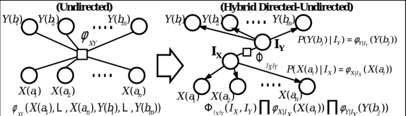
Figure 2: Illustration of a way to factor a potential with two relational atoms,X(ai) and

Y(bj). Our variational method converts an undirected model (left) into a factor model

(right). In the factored model, the distribution is dependent on the new latent variables,IX

andIY.

joint probability defined by a setF of factors on a valuationvof random variables is the

normalization ofQ

f∈_Fwf(v).

An important property of the factor f is that its tupleAf is a disjoint union of sets of

exchangeable random variables1defined as follows:

Definition(Exchangeable Random Variables). A finite or infinite sequenceX(a1),· · ·,X(an)

of random variables areexchangeable, when for any finite permutationπ() of the indices

the joint probability distribution of the permuted sequenceX(a_π(1)),· · ·,X(aπ(n)) is the same

as the joint probability distribution of the original sequence.

A relational atom refers a set of exchangeable random variables. For example, a

potential with two relational atoms (or just atoms) X() and Y() can be represented as

follows:φ(X(a1),· · ·,X(an),Y(b1),· · ·,Y(bm)).

3. Relational Variational Lemma

A potential with a large number of random variables introduces inference difficulties of

three kinds. First, it may require a large number of parameters to represent the probability density. Second, it is hard to learn the potential accurately unless a large number of training examples are given. Third, it requires a substantial amount of computations to marginalize out random variables participating in such potentials. To address these issues, we propose a model-factorization based variational method.

3.1 De Finetti-Hewitt-Savage’s Theorem

Before introducing our variational method, we review de Finetti’s theorem [6] which shows that any probability density function (pdf) of an infinite number of binary exchangeable 1. Note that, our representation is a general representation than existing relational models [15, 7, 19, 13, 21, 3, 11, 2] in terms of expressiveness. That is, not all potential withs exchangeable variables in RHMs can be represented by existing models either based on Parfactors [15, 7, 13, 3, 11, 2] or MNLs [19, 21].

random variables can be represented by a mixture of independent and identically

dis-tributed (iid) Bernoulli random variables (RVs) and the density over the RVs:

lim n→∞p(X(a1), · · ·,_X(an))= Z 1 0 θtn₍₁−θ₎n−tn·Φ_X(θ_{) d}θ,

whentn = PiX(ai). This observation is extended to multi-valued RVs by Hewitt-Savage

theorem. lim n→∞p(X(a1), · · ·,_X(an))= Z n Y i=1 φX|_IX(X(a_i))·Φ_X(I_X) dI_X (1)

whereIX is a new latent variable which chooses a distributionφX(·|IX) for the iid

multi-valued Bernoulli RVs.2_{. We also useφ}

X|_IX(.) to refer to φ_X(.|I_X). Figure 1 illustrates an

example of a variational form. The parameters of the potential (e.g. entries in the condi-tional density table (CDT)) could be substantially reduced by the factorization. Note that,

the graphical model on the right hand side requires only a representation ofφX|_IX and the

densityΦXoverIX.

This variational method is exact only if there is an infinite number of RVs. Thus, it is natural to analyze the error when we have a finite number of RVs. Before analyzing this

error, we define a termn-extendible:

Definition (n-extendible). pn(X(a1,· · ·,X(an)), any pdf with n exchangeable RVs, is n-extendible when the following holds: (1) there is p_n(X(a1),· · ·,X(an),X(an+1),· · ·,X(an)),

a pdf with nexchangeable RVs (n < n); and (2)pn is the marginal distribution ofpn (i.e.

eliminating (n−_{n) RVs).}

Lemma 1(Diaconis and Freedman [9]). If pn(X(a1),· · ·,X(an)), any pdf with n exchangeable RVs, is n-extendible, then the total variation distancek · k_{between pnand the variational form in the} Hewitt-Savage’s theorem is bounded as follows: (i) when X(ai)are discrete RVs with a domain of cardinality c (e.g. c=2 for binary RVs),

pn− R Qn i=1φX|_IX(X(a_i))·Φ_X(I_X) dI_X ≤ 2cn n ; (ii) when X(ai)are continuous RVs, pn− R Qn i=1φX|_IX(X(a_i))·Φ_X(I_X) dI_X ≤ n(n−₁₎ n .

The total variation distance isk_p−_qk =_{supA∈B(p(A)}−_{q(A)) when}B_{is a class of Borel}

sets.

3.2 Factoring Potentials with Multiple Atoms

De Finetti’s theorem and Heweitt-Savage’s theorem of the previous section are applicable only to potentials with a single relational atom. In this section, we present our key new result that establishes variational methods for RHMs. Lemma 5 provides a result on potentials with an infinite number of objects. Lemma 6 provides an error bound on a single variational step, and Theorem 4 provides an error bound for our relational variational method in RHMs.

2. In general, the right hand side of Equation (1) isR Qni=1φX(X(ai)|IX)·ΦX( dIX). When the distributionΦXhas

a density, it is possible to replaceΦX( dIX) withΦ(IX) dIX. Here, we only consider distributions of which

Lemma 2 (Existence of a variational factor). For pn,m(X(a1),· · ·,X(an),Y(b1),· · ·,Y(bm)), a potential with two relational atoms in a RHM, there are two new latent variables, IXand IY, and a new potential of two variables pXYsuch that the following holds,

lim n,m→∞pn,m(X(a1), · · ·,_X(an),_Y(b1),· · ·,_Y(bm))= Z ΦXY(IX,IY) n Y i=1 φX|_IX(X(a_i)) m Y j=1 φY|_IY(Y(b_j)) dI_XdI_Y.

We extend the previous framework and define the term (n,m)-extendible. It then

allows us to derive an error analysis forpn,m3:

Definition ((n,m)-extendible). pn,m(X(a1),· · ·,X(an),Y(b1),· · ·,Y(bm)), any pdf with n

ex-changeable RVs ofX() andmexchangeable RVs ofY() is (n,m)-extendiblewhen it holds

followings: (1) there is pn,m(X(a1),· · ·,X(an),Y(b1),· · ·,Y(bm)), a pdf with n exchangeable

RVs ofX(·_{) andmexchangeable RVs ofY(}·_{) (n} < _n,_m < _{m); and (2)pn,m is the marginal}

distribution ofp_n,m(i.e. eliminating (n−_{n) RVs ofX() and (m}−_{m) RVs ofY()).}

Lemma 3 (Error of a variational factor). If pn,m(X(a1),· · ·,X(an),Y(b1),· · ·,Y(bm)), any pdf with two relational atoms, in a RHM is (n,m)-extendible, the total variation distance of pn,mand the piid(n,m) (the variational form in Lemma 5) is bounded as follows: (i) when RVs of X()and Y()

are discrete with domains of cardinality cx and cy respectively,

pn,m−piid(n,m) ≤ 2cxn n + 2cym m ; (ii) when X(·_{) are discrete RVs with a domain of cardinality cx and Y(}·_{) are continuous RVs,}

pn,m−piid(n,m) ≤ 2cxn n + m(m−₁₎

m ; (iii) when X()and Y()are continuous RVs,

pn,m−piid(n,m) ≤ n(n−₁₎ n + m(m−₁₎ m .

For pdfs with more than two relational atoms (e.g. p(X(a1),· · ·,X(an),Y(b1),· · ·,Y(bm), Z(c1),· · ·,Z(cu)), it is natural to extend Lemma 6 as follows: The total variation distance is

bounded by the sum of the variation distances for all relational atoms in the potential.

Theorem 4(Variational error of a RHM). For each factor fiin a RHM F, its potential pi is a pdf (or normalized), and the total variation distance between pfi and its variational form piid(i) is bounded byi, then the total variation distance between the joint distribution of G and its variational form is bounded by 1_zP

ii when z is the normalizing constant ofQipfi.

We provide proofs of Lemma 5, Lemma 1, and Theorem 4 in Appendix A.1, A.2 and A.3.

4. How to Find a Variational RHM?

The previous section concerned the existence of a relational form that represents or

ap-proximates our original distribution well. In this section4we address the question of how

to convert potentials (e.g. pn) into a variational lifted relational form.

When a given potential is ∞_{-extendible, it is possible to derive the cdf FX(IX) on IX}

analytically as follows [8]:FX(IX)=limn→∞1_n|{i|X(a_i)≤I_X}|. For example, relational Models

3. We usepn,mto refer the original (unfactored) potentialφXY, andpiid(n,m)to refer the factored model.pn,mand

piid(n,m)are the pdfs of the potential formsφn,mandφiid(n,m), respectively. The difference between potential

and pdf is that a pdf is integrated into 1 while a potential is not.

with continuous RVs (e.g. pairwise Gaussian [3] and Gaussian processes [4, 23]) allow such

analytical derivations [12]5_.

Unfortunately, it is not possible to use such derivations in general because some

poten-tials are not∞_{-extendible, so limn→∞}1

n|{i|X(ai)≤IX}|is not defined.

In the following we focus on providing solutions for non-trivial problems which have no analytical solution. Here, we provide solutions for discrete models first, then for continuous models.

4.1 Lifting Discrete Variables

When an RHM includes potentials with discrete RVs, we need to find a density function

ΦX(IX)over the iid Bernoulli RVs of parametersIX. We start with binary RVs. To solve the

problem, we formulate Equation (1) as follows: arg max ΦX(IX) φh( hX)− Z ΦX(IX)· f_B(hX;n,IX) dIX ≈ _{arg max} h_(w 1,i1X),···,(wk,ikX)i φh(hX)− k X l=1 wl·f_B(hX;n,ilX) , (2) wherePk

l=1wl=1.φh(hX) in Equation (2) is the value-histogram representation introduced

in previous lifted-inference methods [7, 13]. Thus, given values ofnRVs,X(a1),· · ·,X(an), the

value histogram is a vectorhXwithhXv =|{i:X(ai)=v}|for eachvin RVs’ range. WhenhX

is the value histogram ofX,φn(X(a1),· · ·,X(an))=φh(hX). fB(hX;n,IX)= _hn_X1I_XhX1(1−IX)n−hX1

is the pdf of the binomial distribution.

The approximation in Equation (2) is due to our incremental iterative algorithm,

choos-ing an empiricalkthrough iterations.6

For binary RVs,φX|_IXis the Bernoulli (distribution) withI_Xl as a parameter (i.e. P(X(aj)=1)=

il_X). Thus,il_Xin Equation (2) is a parameter of the binomial distribution, andwlis the

den-sity on the Bernoulli distributions. That is, the problem is to find a mixture of binomial distributions.

For multi-valued variables, φX|_IX is the multi-valued Bernoulli, i.e. Categorical

distri-bution. The problem is to find a mixture of multinomial distributions f_M:

arg max h_(w1,i1 X),···,(wk,ikX)i φh(hX)− k X l=1 wl·f_M(hX;n,ilX) (3)

For potentials with two or more relational atoms, it can be formulated as follows: arg max h_(w1,i1 X,i1Y),···,(wk,ikX,ikY)i φh(hX,hY)− k X l=1 wl·f(hX;n,ilX)·f(hY;m,ilY) , (4)

where f is either the binomial or the multinomial which depends on the range of RVs.

We learn the parameters (e.g. (w,iX) in Equation (2)) from the original potentialφusing

an EM algorithm that solves Equations (2), (3) and (4).7 _{Normally, such EM algorithms}

assume thatkis known or given. Because the assumption does not hold for this case, we

increasekwith an incremental EM algorithm until the error converges. The achieved error

5. For Gaussian processes with an infinite number of exchangeable RVs, the mean of RVs follows a Gaussian distribution. Given a mean, each RV also follows a Gaussian distribution.

6. Notice that this is applicable even when there is no analytical derivation for the model 7. EM algorithms are used to learn parameters for mixture models, e.g. [22, 5, 18].

withkcomponents is the empirical error of the theoretical one in Lemma 6. It is well known that EM algorithms derive a close-to-optimal mixture model when components in the true density are well separated (e.g. |µ_i−µ_j|> σ2

i +σ2j for Gaussian mixtures) [22].

4.2 Lifting Continuous Variables

For a potentialφwith RVs in a continuous domain, finding the variational lifted relational

form requires additional considerations for non-parametric densities. The variational form for continuous domains is possibly a mixture of non-parametric densities. Here, we

gen-erate samples from the input potentialφ, then learn a mixture of non-parametric densities.

Equation (1) for discrete potentials is adapted to continuous and hybrid potentials as follows: arg max ΦX(IX) φn(X())− Z ΦX(IX)· n Y j=1 ˆ fIX(X(aj)) dIX ≈ _{arg max} h_(w1,fˆ_i1 X ),···_,(wk,fˆ_ik X )i φn(X())− k X l=1 wl· n Y j=1 ˆ f_il X(X(aj)) , (5)

whereφn(X()) =φn(X(a1),· · ·,X(an)) and ˆfIX represents a non-parametric distribution. To

solve this equation, we generateNsamplesV1_,· · ·,_VN_{from the input potentialφwhereV}j ₌

(v₁j,· · ·,_vj

n), i.e. values ofnRVs. Then, the problem is formulated as the maximum likelihood

estimation (MLE) problem: arg maxh_(w1,_fˆ

i1_X),···,(wk,fˆik_X)i PN t=1ln Pk l=1wl· Qn j=1 fˆil_X(vtj) . We denote by ˆf

i_Xj the kernel density estimator: ˆfilX=

1 nlh Pnl s=1K _x−_vs h when (v1,· · ·,vnl) are

data points that underlie the density andhis the parameter. Here, we use a Gaussian Kernel,

K(x)= √1 2πe

−_x2

2 . It is interesting to note that the kernel density estimator is analogous to the

value histogram of discrete RVs in a sense that frequently observed regions (or bins) have higher probability. In this way, the intuition of the value histogram helps us generalize the method for continuous RVs.

For potentials with two or more relational atoms, the approach can be formulated as follows: arg maxh_(w1,fˆ

i1_X,fˆi1_Y),···,(wk,fˆik_X,fˆik Y )i PN t=1ln Pk l=1wl·Qnj=1 fˆil X(v t Xj) ·Qm j0 =1 fˆil Y(v t Yj0) , where vt

Xj is the value ofj-th RV ofXin thet-th sample, andv

t

Yj0 is the value of j 0

-th RV ofY.

This MLE problem can also be solved by an EM algorithm. There, one of Nsamples

will be used to build one ofkdensities in a maximization (M) step, and the likelihood of

each sample fromkdensities is calculated in an expectation (E) step. With discrete RVs,k

is determined in an incremental way until the variation error converges.

5. Lifted Inference with Variational RHM

Our previous two sections presented methods and error bounds for lifting and factoring complex hybrid relational models. Those results provide variational RHMs in which all potentials are in variational relational lifted forms.

In this section we build on those results and present two algorithms that apply the variational steps above to speed up relational inference algorithms. Sections 5.1 and 5.2 present Lifted Hybrid Variable Elimination on those models. Section 5.3 addresses the case when the resulting model is still too complex for exact inference, and present an MCMC sampling algorithm that samples at a lifted level without grounding unnecessarily.

5.1 Inference with Discrete Variables

A variable elimination (VE) is an inference procedure with following steps: (i) choosing an atom; (ii) finding all potential including the atom; (iii) making a produce of the found potentials; (iv) marginalizing the atom; and (v) repeating the steps until only output atoms remain. We demonstrate the key step in our Lifted Variational VE, Step (iv), with an

example: a potentialφwith two atomsX() andY() andφ0 with a atomY(). Suppose that

the potentials are converted into a variational form as Equation (4). Then the marginal

probability ofIXcan be derived by marginalizing the atomY() out: Phyφh(hx,hy)·φ

0 h(hy) ≈X hy k X l=1 wlf(hx;n,ilX)fB(hy;m,ilY) k0 X l0₌₁ wl0f B(hy;m,il 0 Y)= k X l=1 k0 X l0₌₁ wlwl0         X hy f_B(hy;m,ilY)fB(hy;m,il 0 Y)         f(hx;n,ilX) ≈ k X l=1 k0 X l0₌₁ wlwl0 Z f_N(hy;µ(m,il Y), σ 2 (m,il_Y))fN(hy;µ(m,il0 Y), σ 2 (m,il0 Y) ) dhy ! f(hx;n,ilX)= k X l=1 wY l·f(hx;n,ilX) (6) whenPk l=1wYl =1, wherefN(hy;µ(n,p), σ 2

(n,p)) is a pdf of the Normal distribution with a mean

µ(n,p)(= n·p) and a variance σ2_(n,p)(= n·p·(1−p)), and zl,l0 is the inverse of the normalizing

constant calculated from the product of two Normal pdfs. Equation (6) is the Normal

approximation to Binomial for a largem. Whenmis small, we can keep the value histogram

representation. Then, the marginal density is still represented as a mixture of iid Bernoulli RVs. Note that, other procedures involving more relational atoms hold the property, although the representation may include more components.

Now, we will show that the product of variational forms in Step (iii) can also be

represented as a variational from. Suppose that we have two probabilities forIXof binary

RVs, one from φh(hx,hy) after marginalizing Y() out, and another from φ0_h(hx,hz) after

marginalizingZ() out, i.e. Pk

l=1wYl ·fB(hx;n,i l X) and Pk0 l0₌ 1wZl0·f 0 B(hx;n,il 0

X). Note that, it can

bek,k0 and f_B(hx;n,il_X),f0

B(hx;n,ilX) because the parameters are extracted from different

potentials,φh(hx,hy) andφ0_h(hx,hz). Then, the product of two potentialsφh(hx) andφ0_h(hx)

is as follows: k X l=1 wY l·fB(hx;n,ilX)· k0 X l0 =1 wZ l0·f 0 B(hx;n,il 0 X)= k X l=1 k0 X l0 =1 wY l·w Z l0· X hx f_B(hx;n,ilX)·f 0 B(hx;n,il 0 X) ≈ k X l=1 k0 X l0 =1 wY_l·_wZ l0 Z f_N(hx;µ(n,il X), σ 2 (n,il X) )·_f0 N(hx;µ(n,il0 X), σ 2 (n,il0 X) ) dhx= k X l=1 k0 X l0 =1 wY_l·_wZ l0·z_l,l0f N(hx;µnew, σ2new), (7)

zl,l0 is the inverse of the normalization constant of the product of two Normal pdfs. This

has|_k·_k0_|

Normal components, but there are several way to reduce some of them, which we omit here for lack of space.

5.2 Inference with Continuous Variables

Similar to the discrete cases, we demonstrate Lifted Variational VE for continuous variables

with an example. Assume two potentialsφwith two atomsX() andY(), andφ0with a atom

Y(). Two potentials are represented by a variational form such as in Equation (5). Then

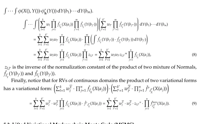
R · · ·R φ_(X(),_Y())·φ0 h(Y()) dY(b1)· · ·dY(bm). Z · · · Z         k X l=1 wl n Y j=1 ˆ f_il X(X(aj)) m Y j0₌₁ ˆ f_il Y(Y(bj 0))                 k0 X l0₌₁ wl0 m Y j00₌₁ ˆ f_il0 Y(Y(bj 00))         dY(b1)· · ·dY(bm) = k X l=1 k0 X l0₌₁ wlwl0 n Y j=1 ˆ f_il X(X(aj)) · m Y j0₌₁ Z ˆ f_il Y(Y(bj 0))· fˆ il_Y0(Y(bj0)) dY(bj0) ! = k X l=1 k0 X l0₌₁ wlwl0 n Y j=1 ˆ f_il X(X(aj)) m Y j0₌₁ zl,l0= k X l=1 k0 X l0₌₁ wlwl0z_l,l0m n Y j=1 ˆ f_il X(X(aj)), (8)

zl,l0 is the inverse of the normalization constant of the product of two mixture of Normals,

ˆ

f_il Y(Y(bj

0)) and ˆf

ic_Y(Y(bj0)).

Finally, notice that for RVs of continuous domains the product of two variational forms has a variational form:

Pk l=1wYl · Qn j=1 fˆil X(X(aj)) · Pk0 l0 =1wZl0 · Qn j=1 fˆ0il0 X(X(aj)) = k X l=1 k0 X l0₌₁ wY l ·w Z l0 n Y j=1 ˆ f_il X(X(aj)) · _fˆ0 il0 X(X(aj))= k X l=1 k0 X l0₌₁ wY l ·w Z l0·z_l,_l0n· n Y j=1 ˆ fnew il_X,l0 (X(aj)). (9)

5.3 Lifted Variational Markov chain Monte Carlo (MCMC)

When lifted relational variational relational models are still too complex for Lifted Varia-tional VE, we can apply MCMC on the results of our lifting operatios above. In general, MCMC sampling is composed of five steps: (i) choosing a RV to sample; (ii) calculating the conditional probability of each potential using assignments of neighboring RVs; (iii) build-ing a probability a density with the product of the conditional probabilities; (iv) choosbuild-ing an assignment from the density; and (v) repeating until some conditions are met.

Here, the main steps are Steps (ii), (iii), and (iv). Step (ii) is a subset of the marginalization procedure in Equations (6) and (8). Step (iii) can be derived in a straightforward manner from Equations (7) and (9).

Thus, we focus our attention on Step (iv). Recall that we choose a component according

to the results in Equations (7) and (9). Essentially, we choose one component for X()

proportional towY

l ·wZl0·z_l,_l0 out of|k| · |k

0_|

Normal pdfs. With Lifted MCMC (compared with ground MCMC) we also need to choose a tuple of indices for all potentials which include

X(). For example, when we choose the (l,l0)-th component, we assign a tuple of indices

(il X,il

0

X) forIX. Then, the first indexilXwill be used to calculate the conditional probability

ofφh(hy) inφh(hx,hy), andil 0

Xwill be used inφh(hx,hz).

6. Experimental Results

We provide experimental results about the number of components in the lifted relational

variational form, and the computational efficiency of the lifted inference. First, we address

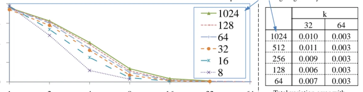
the question: to what degree can we reduce the number of components in the variational form. To examine this, we build a simulation with a single atom of 100 RVs. We ran-domly choose 30 mixtures of Binomials (various numbers from 8 to 1024) per parameters. Figure 3 shows the average variational distance of the target density and our variational

0 0.2 0.4 0.6 0.8 1 2 4 8 16 32 64 1024 128 64 32 16 8

k: the number of components used in the variational form

T o tal v ar iatio n d is tan ce

The number of components in the targeting density

k 32 64 1024 0.010 0.003 512 0.011 0.003 256 0.009 0.003 128 0.006 0.003 64 0.007 0.003

Total variation error with two k values, 32 and 64

Figure 3: The variation distance of our lifted relational variational model with k

compo-nents. Even if a target density has a larger number of components, we obtain a close

approximate density with a reasonably smallk.

model derived from our EM algorithm. It shows that with a significant fewer number of

components (e.g. 32) the variation distance becomes reasonable small (≤₀._{01). When we}

increase the number RVs (e.g. 200 and 1000), the results are consistent with the plot. Thus, it shows that it is a reasonable idea to use the incremental iterative algorithm to learn the parameters. E rr o r of p o steri o r d is tri b u ti o n Number of samples 0 0.5 1 1.5 2 0 25000 50000 75000 100000 Ground(16) Ground(1) Ground(8) Lifted(100) Ground(4) Lifted(16) houses

(a) The accuracy of samplings

T ime pe r sa mpl ing s te p ( ms ec ) Number of houses 0 2000 4000 6000 8000 10000 0 200 400 600 800 1000 Ground Lifted

(b) The sampling time

Figure 4: Figure (a) compares the accuracy of posterior distributions of our lifted MCMC and the ground MCMC with various numbers of houses. ‘()’ indicates the number of houses (e.g. ‘Ground(16) is a ground MCMC with 16 houses). Figure (b) shows the average sampling time per each time step with various number of houses.

Second, we examine the computational improvement of our algorithms compared with

ground algorithms. We compare the accuracy and the efficiency of our lifted MCMC

algorithm with a traditional (ground) MCMC algorithm on a linear Gaussian model. The

model is composed of two relational atoms Job() andHPC() (orHousePriceChange()). The

φJob is the Bernoulli distribution with a parameter pJob. The φHPC is a mixture of two

Gaussians: wDNN(−0.3, σ2_DN)+wUPN(0.1, σ2_UP). Then, the parameters of two atoms are

related by the following linear Gaussian: Φ(φJob, φHPC)=N(pjob−wDN, σ2_JH). Figure 4a shows

the accuracy of the two algorithm given the same number of samples. That is, it measure the ratio of error to estimate a probability density of an eventx,|_ptrue(x)−_pMCMC(x)|/_ptrue(x).

It shows that the ground MCMC suffer from the curse of dimensionality, when the search

4b represent the sampling time per step with different number of RVS (e.g. the number of houses).

Finally, we find an exemplar model in Republican River Compact Administration

(RRCA) dataset.8 RRCA Ground Water Model (RRCA Model) is to determine the amount,

location, and timing of streamflow depletions to the Republican River caused by various

effects such as well pumping. However, the state-of-the-art RRCA model is not always

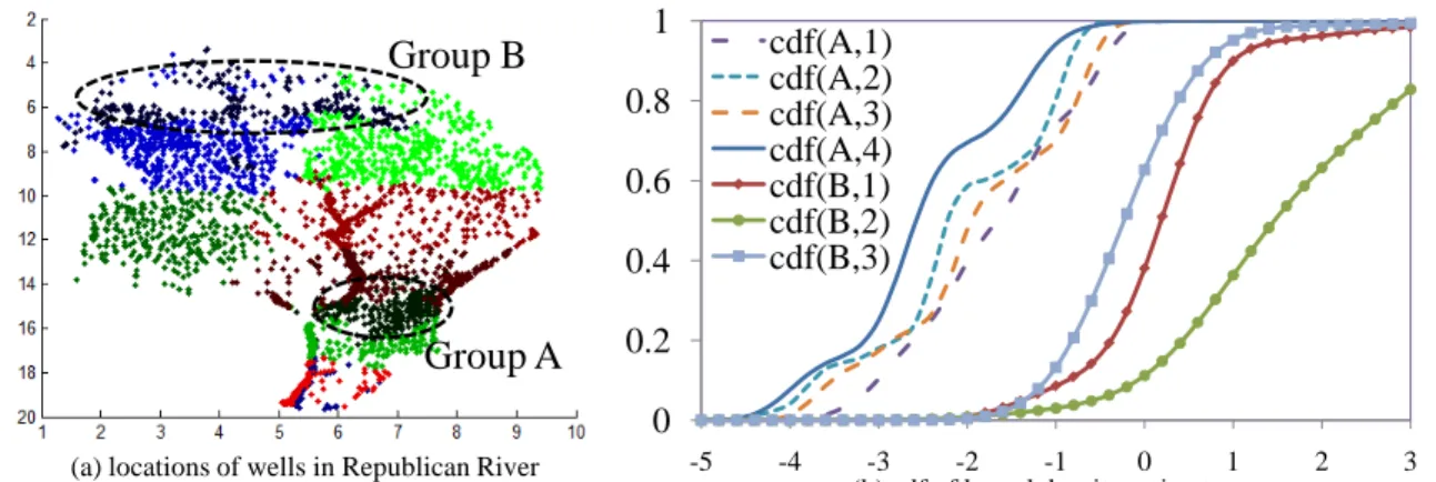
accurate. Thus, it is required to compensate the error (or residual) of estimation in each well. In a preliminary experiment, we cluster the locations of wells into 10 groups which shows a similar (approximately exchangeable) residuals pattern. Then, we select two of regions, groups (or atoms) A and B. Figure 5 shows identified cdfs for each groups. As the discrete case, with only small number of components (4 for A and 3 for B), we can represent the mixtures of cdfs. That is, there is no substantial improvement of the likelihood when we increase the number of mixtures.

0 0.2 0.4 0.6 0.8 1 -5 -4 -3 -2 -1 0 1 2 3 cdf(A,1) cdf(A,2) cdf(A,3) cdf(A,4) cdf(B,1) cdf(B,2) cdf(B,3)

(b) cdf of kernel density estimators

Group A

Group B

(a) locations of wells in Republican River Compact Administration (RRCA) dataset

Figure 5: Figure (a) shows the locations of clustered wells in the regions. Figure b) represented Gaussian kernel density estimators learned by our EM algorithm.

7. Conclusion

We propose an efficient lifted inference algorithm for RHMs with discrete variables and

continuous variables. With a variational method, we reduce the time and space complexity of handling potentials with a large number of RVs. It is the first variational lifted inference algorithm which is generally applicable to various types of potentials in hybrid domains. Thus, it is a scalable algorithm which can be used for intractable hybrid graphical models with a large number of RVs.

8. Acknowledgement

This work is supported by NSF EAR 09-43627 EA.

Appendix A. Additional Proofs

A.1 Existence of a variational factor

Lemma 5 (Existence of a variational factor). For a potential with two relational atoms in a RHM,φXY(X(a1),· · ·,X(an),Y(b1),· · ·,Y(bm)), there are two new latent variables, IXand IY, and a new potential of two variablesΦXYsuch that the following holds,

lim n,m→∞φXY(X(a1), · · ·,_X(an),_Y(b1),· · ·,_Y(bm))= Z ΦXY(IX,IY) Y i φX|_IX(X(ai)) Y j φY|_IY(Y(bj))dIXdIY.

Proof. Given the potential φXY, suppose that the value of X(a1),· · ·,X(an) are assigned

with constants (c1,· · · ,cn). Then, from the Hewitt-Savage’s theorem, it can be factored as

follows. lim m→∞φXY(c1, · · · ,_cn,_Y(b1),· · · ,_Y(bm)) = Z ΦY(IY) Y j φY|_IY(Y(b_j))dI_Y. (10)

Note that,ΦY(IY) is a pdf overIY. That is,ΦY(cY) is a constant density for an assignment,

IY = cY. By an assignment fornRVs (X(ai)· · ·,X(an)), the constant densityΦY(cY) can be

represented as a function of thenRVs for a further factoring.

lim n→∞ΦY(cY) = _nlim→∞φcY(X(a1), · · ·,_X(an)) = Z ΦXcY(IX) Y i φX|_IX(X(a_i))dI_X

To represent general cases, it is enough to allow that thecYinΦXcY(IX) is parameterized by

IY(ΦXY(IX,IY)) as follows. lim n→∞ΦY(Y)= Z ΦXY(IX,IY) Y i φX|_IX(X(a_i))dIX. (11)

When we substitute ΦY(Y) in Equation (10) with Equation (11), the following result is

derived. Z ΦXY(IX,IY) Y i φX|_IX(X(a_i)) Y j φY|_IY(Y(b_j))dI_XI_Y.

A.2 Error of a variational factor

Lemma 6 (Error of a variational factor). If pn,m(X(a1),· · ·,X(an),Y(b1),· · ·,Y(bm)), any pdf with two relational atoms, in a RHM is (n,m)-extendible, the total variation distance of pn,mand the piid(n,m) (the variational form in Lemma 5) is bounded as follows: (i) when RVs of X()and Y()

are discrete with domains of cardinality cx and cy respectively,

pn,m−piid(n,m) ≤ 2cxn n + 2cym m ; (ii) when X(·_{) are discrete RVs with a domain of cardinality cx and Y(}·_{) are continuous RVs,}

pn,m−piid(n,m) ≤ 2cxn n + m(m−₁₎

m ; (iii) when X()and Y()are continuous RVs,

pn,m−piid(n,m) ≤ n(n−₁₎ n + m(m−₁₎ m .

Proof. We need to review the proof for a single atom in [9]. It shows that a ¯n-extendible

pdf, pn, can be represented by a mixture of extreme pdf (e.g. pn = Pewepe). Here, an

extreme pdfpeis a distribution ofndraws made at random without replacement from an

urn,U, which contains ¯nballs marked by one ofccolors. Letea unique marking inU. The

variation distance of each extreme pointpeand its variational formQiφX|_e(X_i) is bounded

≤ 2cn

¯

n for discrete RVs. .

For a distribution with the multiple atoms, each extreme point corresponds to the joint

distribution of ndraws from one urn, UX of ¯n balls, andmdraws from another urn,UY

of ¯m balls, respectively. The draws can be done independently for each urn. Thus, an

extreme pdf (e.g. pex,ey) can be represented as the product of independent extreme pdfs

(e.g. pex ·pey). The variation distances of variational forms ofpex andpey are respectively

bounded. WLOG, we can represent the errors withxandy,

pex − Y i φX|_ex(X_i) ≤_x, pey− Y j φY|_ey(Y_j) ≤_y. Then, pex ·pey − Y i φX|_ex(X_i)· Y j φY|_ey(Y_j) ≤_x+_y.

Thus, total variation distance between two densities, pn,m andpiid(n,m) is bounded by the

product of the sum of two error bounds and the normalization constant (1_z). Note that, the

product of two pdfs may not be a pdf without a normalization constant.

A.3 Variational error of a RHM

Theorem 7(Variational error of a RHM). For each factor fi in a RHM F, its potential pi is a pdf (or normalized), and the total variation distance between p_fi and its variational form p_iid(i) is bounded byi, then the total variation distance between the joint distribution of F and its variational form is bounded by 1_zP

ii when z is the normalizing constant ofQipfi.

Proof. WLOG, we refer relational atoms in F as X1,· · ·,XN when N is the number of

relational atoms. Here, we shorten the jth rv of theith atomXi(aj) intoX_ij. ni refers to the

number of RVs in theithatom (i.e. X1_i,· · ·,X_ini).

The joint distribution of all relational atoms can be written as the product of pdfs in

factors. Thus, it is possible to build an aggregated pdf p with all relational atoms as

arguments (unfactored form).

p(X1₁,· · ·,_Xn1 1 ,X 1 2,· · ·,X n2 2 , · · · ,X 1 N,· · ·,X nN N ).

Suppose thatp_iid(i)is the variational form (as shown in Lemma 5) ofp_fi. Let the error caused

by each atom as0_j (1≤ _j ≤_{N). Then, total variation distance}k_pf

i −piid(i)kis bounded by

P

j=1,···,_N 0

j.

Now, we prove that P

j=1,···_,N0_j ≤ P_i=1,···_,|_F|i (|F| is the number of factors). For each

P

js.tXj∈fi 0

j). Given the fact that each relational atom is included in a factor at least once,

P j 0 j≤ P ii.

Appendix B. Analysis of the Lifted-MCMC Algorithm

In this section, we will present the details of the Lifted-MCMC algorithm. Then, we will

show the correctness and computational complexity of the Lifted-MCMC algorithm.9

B.1 Correctness

We prove that ourLifted-MCMC converges to a correct stationary distribution, if a Gibbs

sampling algorithm over a grounded RHM (e.g. [21]) converges to the stationary distribu-tion.

Lemma 8. If a Gibbs sampling algorithm over grounds variables in a RHM converges to a stationary distribution, theLifted-MCMCalgorithm converges to the stationary distribution.

Proof. To prove the convergence, we prove that theLifted-MCMCisirreduciblewhich means

that the Markov Chain can move between any pair of points. Then, we prove that

Lifted-MCMCis ergodic.

We prove theirreducibilityby contradiction. Assume that there is a sampleS_L0=(IX1 =

d0₁,· · ·,_IX

N =d

0

N) which can not reach to another sampleSLt=(dt1,· · ·,d

t

N). Suppose there is a

map from each distributiondito a sample for corresponding RVs (Si=(Xi(a1),· · ·,Xi(a|_Xi|))).

The map finds the most likely values for the RVs from the chosen distribution (e.g. di). In

this way,S_L0andS_Ltare mapped toS_G0=(S0₁,· · ·,_S0

N) andSGt=(St1,· · · ,S

t

N), respectively.

The Gibbs sampler over ground RVs always finds a path fromS0

G andSGt because it

is irreducible. (Otherwise, it can not converge to the stationary distribution.) WLOG, we

assign the length of path astso that we can refer a sample in a path asS_Gj=(S₁j,· · ·,_Sj

N)

when 0≤ _j≤_{t. Now, for the jth sample in the path, we can define an inverse map which}

finds the most likely distributiond_ij for each relational atom from the sample of ground

RVsS_ij.

In that way, we can prove that the Lifted-MCMCcan move fromS_Lj toS_Lj+1 for all j.

Suppose that, theith latent variabled_ij is changed tod_ij+1 by the inverse map. Then, the

transition probability of the movement is determined by other latent variables. That is,

the transition probability is positive whenever two samplesS_Gj andS_Gj+1are reflected in

finding potentialsΦ(). Because the factorization is exact, the transition probability between

jandj+1 are positive for all j. It contradicts to the assumption. Thus, theLifted-MCMCis

irreducible.

Any finite state irreducible Markov Chain is ergodic. Based on the two properties

(irreducibleandergodic),Lifted-MCMCconverges to the stationary distribution.

Thus, when Ground Gibbs sampling converges to a correct solution,Lifted-MCMCalso

converges to the correct solution.

9. Note that, the proof is about the convergence Lifted-MCMC algorithm is converged to the solution of a ground Gibbs sampling algorithms. The solution may incdlue the error caused by the variational form represented in Theorem 7.

B.2 Complexity

Now, we analyze the computational complexity and memory requirement of

Lifted-MCMCalgorithm because other two algorithms are one time batch procedures. We useΩ

to refer a set of all ground RVs. For each relational atomXi,|Xi|refers the number of all

ground RVs in the atom. That is,U={_Xi|_Xi ∈ _f,_f ∈_F}_{when F is a set of factors for a RHM.}

Lemma 9. The computational complexity of MCMC with ground RVs is O(n· |Ω|_{). The space} complexity is O(exp(P

Xi∈F|Xi|)), such that arg maxf

P

Xi∈F|Xi|. ( f is a factor that includes the largest number of ground RVs)

Proof. The computational complexity is straightforward. The space complexity is deter-mined by a factor that includes the largest number of ground RVs. That is, the size of CPT

in the factor is exponentially proportional tothe number of all ground RVsin the factor,

g.

Theorem 10. The computational complexity of Lifted-MCMCis O(n· |_X|_{). The complexity is} O(exp(|{_Xi|_Xi ∈ _f}|_{)), such that arg maxf}|{_Xi|_Xi ∈ _f}|_{. ( f is a factor that includes the largest} number of relational atoms)

Proof. The computational complexity is also straightforward. The space complexity is

determined by a factor that includes the largest number of relational RVs, because

Lifted-MCMCdoes not generate samples for ground RVs. The size of CPT in the factored factor

is exponentially proportional tothe number of relational atomsin the factor, f.

B.3 Accuracy

To solve inference problems, our lifted algorithm requires much less number of samples than previous Gibbs sampling algorithm over ground RVs because it runs on a smaller sampling space. Here, we provide a proof for the faster convergence of our algorithm, so that it provides a accurate sampling given a limited resource (e.g. limited number of samples).

Here, we calculate the total variation distance between the approximationφapproxand

the target distributionφtargetas follows.

X X(a1),···,X(an) φtarget(X(a1),· · ·,X(an))−φapprox(X(a1),· · ·,X(an))

Theorem 11. After convergence to the stationary distribution, the distribution error of Lifted-MCMCis bounded by_Nk +P

iiwhen N is the number of samples,φtargetis factored by k mixtures, andi is the error bound of each factor fi in a RHM. After convergence, the error of any ground based Gibbs sampling is bounded by exp_N(n)with n ground variables and N samples.

Proof. Each sample at time t follows the stationary distribution because they are already

converged. Thus, we focus on the error to estimate theφtarget.

When the factorization is exact, for each k distributions of latent variables, the error

of density function is bounded by _N1 (i.e. |Φtarget_(i)−ΦLifted_(i)| ≤ 1

Lifted-MCMCover all possible values as follows. X X(a1),···,X(an) |φ_target(X(a1),· · ·,_X(an))−φ_Lifted(X(a1),· · ·,_X(an))| = X X(a1),···,X(an) X i=1,···,_k Y X(ai) φXi(X(ai))|Φtarget(i)−ΦLifted(i)| = X i=1,···,_k |Φtarget_(i)−ΦLifted_(i)| X X(a1),···,X(an) Y X(ai) φXi(X(ai)) = X i=1,···,_k |Φtarget_(i)−ΦLifted_(i)| ≤ k N

When the factorization is not exact, the error is an addition of _Nk andP

iiin Theorem 7.

In the ground case, the error of density function is also bounded by _N1 for each value

of RVs. |φ_target(x1,· · ·,_xn)−ΦGround_(x1,· · ·,_xn)| ≤ 1

N. The error ofGround-MCMCover all

possible valuesexp(n) is as follows,

X X(a1),···,X(an) |φ_target(X(a1),· · ·,_X(an))−φ_Ground(X(a1),· · ·,_X(an))| ≤ X X(a1),···,X(an) 1 N = exp(n) N

Theorem 11 shows how the cardinality of sampling space affects the error of the

poste-rior distribution. For continuous cases, a similar proof can be applied.

References

[1] B. Ahmadi, K. Kersting, and S. Sanner. Multi-evidence lifted message passing, with

application to pagerank and the kalman filter. InIJCAI, 2011.

[2] Jaesik Choi, Abner Guzman-Revera, and Eyal Amir. Lifted relational kalman filtering. InIJCAI, 2011.

[3] Jaesik Choi, David Hill, and Eyal Amir. Lifted inference for relational continuous

models. InUAI, 2010.

[4] Wei Chu, Vikas Sindhwani, Zoubin Ghahramani, and S. Sathiya Keerthi. Relational

learning with gaussian processes. InNIPS. AAA, 2006.

[5] Sanjoy Dasgupta. Learning mixtures of gaussians. InFOCS, 1999.

[6] B. de Finetti. Funzione caratteristica di un fenomeno aleatorio.Mathematice e Naturale,

0, 1931.

[7] Rodrigo de Salvo Braz, Eyal Amir, and Dan Roth. Lifted first-order probabilistic

inference. InIJCAI, 2005.

[9] P. Diaconis and D. Freedman. Finite exchangeable sequences. Annals of Probability, 0, 1980.

[10] Nir Friedman, Lise Getoor, Daphne Koller, and Avi Pfeffer. Learning probabilistic

relational models. InIJCAI, 1999.

[11] Abhay Jha, Vibhav Gogate, Alexandra Meliou, and Dan Suciu. Lifted inference seen

from the other side : The tractable features. InNIPS, 2010.

[12] J. F. C. Kingman. Uses of Exchangeability.The Annals of Probability, 6(2):183–197, April

1978.

[13] Brian Milch and Stuart J. Russell. First-order probabilistic languages: Into the

un-known. InILP, 2006.

[14] Raymond Ng and V. S. Subrahmanian. Probabilistic logic programming.Inf. Comput.,

101(2), 1992.

[15] Hanna Pasula, Bhaskara Marthi, Brian Milch, Stuart J. Russell, and Ilya Shpitser.

Identity uncertainty and citation matching. InNIPS, 2002.

[16] Avi Pfeffer, Daphne Koller, Brian Milch, and Ken T. Takusagawa. Spook: A system for

probabilistic object-oriented knowledge representation. InUAI, 1999.

[17] David Poole. First-order probabilistic inference. InIJCAI, 2003.

[18] Carl E. Rasmussen and Zoubin Ghahramani. Infinite mixtures of Gaussian process

experts. InNIPS, 2002.

[19] Matthew Richardson and Pedro Domingos. Markov logic networks.Machine Learning,

62(1-2), 2006.

[20] Parag Singla and Pedro Domingos. Lifted first-order belief propagation. In AAAI,

2008.

[21] Jue Wang and Pedro Domingos. Hybrid markov logic networks. InAAAI, 2008.

[22] Lei Xu and Michael I. Jordan. On convergence properties of the em algorithm for

gaussian mixtures. Neural Computation, 8:129–151, 1995.

[23] Zhao Xu, Kristian Kersting, and Volker Tresp. Multi-relational learning with gaussian