Directed Bee Colony Optimization Algorithm to Solve the Nurse Rostering Problem

Research Article

Directed Bee Colony Optimization Algorithm to

Solve the Nurse Rostering Problem

M. Rajeswari,

J. Amudhavel,

Sujatha Pothula,

and P. Dhavachelvan

2_{Department of CSE, KL University, Andhra Pradesh, India}

Correspondence should be addressed to M. Rajeswari; [email protected]

Received 26 October 2016; Revised 6 January 2017; Accepted 1 March 2017; Published 4 April 2017

Academic Editor: Reinoud Maex

Copyright © 2017 M. Rajeswari et al. This is an open access article distributed under the Creative Commons Attribution License, which permits unrestricted use, distribution, and reproduction in any medium, provided the original work is properly cited. The Nurse Rostering Problem is an NP-hard combinatorial optimization, scheduling problem for assigning a set of nurses to shifts per day by considering both hard and soft constraints. A novel metaheuristic technique is required for solving Nurse Rostering Problem (NRP). This work proposes a metaheuristic technique called Directed Bee Colony Optimization Algorithm using the Modified Nelder-Mead Method for solving the NRP. To solve the NRP, the authors used a multiobjective mathematical programming model and proposed a methodology for the adaptation of a Multiobjective Directed Bee Colony Optimization (MODBCO). MODBCO is used successfully for solving the multiobjective problem of optimizing the scheduling problems. This MODBCO is an integration of deterministic local search, multiagent particle system environment, and honey bee decision-making process. The performance of the algorithm is assessed using the standard dataset INRC2010, and it reflects many real-world cases which vary in size and complexity. The experimental analysis uses statistical tools to show the uniqueness of the algorithm on assessment criteria.

1. Introduction

Metaheuristic techniques, especially the Bee Colony Opti-mization Algorithm, can be easily adapted to solve a larger number of NP-hard combinatorial optimization problems by combining other methods. The metaheuristic method can be divided into local search methods and global search meth-ods. Local search methods such as tabu search, simulated annealing, and the Nelder-Mead Methods are used to exploit search space of the problem while global search methods such as scatter search, genetic algorithms, and Bee Colony Optimization focus on the exploration of the search space area [1]. Exploitation is the process of intensifying the search space; this method repeatedly restarts searching for each time from a different initial solution. Exploration is the process of diversifying the search space to evade trapping in a local optimum. A hybrid method is used to obtain a balance between exploration and exploitation by introducing local search within global search to obtain a robust solution for the

NRP. In a previous study, the genetic algorithm was chosen for global search and simulated annealing for a local search to solve the NRP in [2].

In swarm intelligence, the natural behavior of organisms will follow a simple basic rule to structure their environment. The agents will not have any centralized structure to control other individuals; it uses the local interactions among the agents to determine the complex global behavior of the agents [3]. Some of the inspired natural behavior of swarm intelli-gence comprises bird flocking, ant colony, fish schooling, and animal herding methods. The various algorithms include the ant colony optimization algorithm, genetic algorithm, and the particle swarm optimization algorithm [4–6]. The natural foraging behavior of honey bees has inspired bee algorithm. All honey bees will start to collect nectar from various sites around their new hive, and the process of finding out the best nectar site is done by the group decision of honey bees. The mode of communication among the honey bees is carried out by the process of the waggle dance to inform hive mates about Volume 2017, Article ID 6563498, 26 pages

the location of rich food sources. Some of the algorithms which follow the waggle dance of communication performed by scout bees about the nectar site are bee system, Bee Colony Optimization [7], and Artificial Bee Colony [8].

The Directed Bee Colony (DBC) Optimization Algorithm [9] is inspired by the group decision-making process of bee behavior for the selection of the nectar site. The group decision process includes consensus and quorum methods. Consensus is the process of vote agreement, and the voting pattern of the scouts is monitored. The best nest site is selected once the quorum (threshold) value is reached. The experimental result shows that the algorithm is robust and accurate for generating the unique solution. The contribution of this research article is the use of a hybrid Directed Bee Colony Optimization with the Nelder-Mead Method for effective local search. The authors have adapted MODBCO for solving multiobjective problems which integrate the fol-lowing processes: At first a deterministic local search method, Modified Nelder-Mead, is used to obtain the provisional opti-mal solution. Then a multiagent particle system environment is used in the exploration and decision-making process for establishing a new colony and nectar site selection. Only few honey bees were active in the process of decision-making, so the energy conservation of the swarm is highly achievable.

The Nurse Rostering Problem (NRP) is a staff scheduling problem that intends to assign a set of nurses to work shifts to maximize hospital benefit by considering a set of hard and soft constraints like allotment of duty hours, hospital regulations, and so forth, This nurse rostering is a delicate task of finding combinatorial solutions by satisfying multiple constraints [10]. Satisfying the hard constraint is mandatory in any scheduling problem, and a violation of any soft constraints is allowable but penalized. To achieve an optimal global solution for the problem is impossible in many cases [11]. Many algorithmic techniques such as meta-heuristic method, graph-based meta-heuristics, and mathematical programming model have been proposed to solve automated scheduling problems and timetabling problems over the last decades [12, 13].

In this work, the effectiveness of the hybrid algorithm is compared with different optimization algorithms using performance metrics such as error rate, convergence rate, best value, and standard deviation. The well-known combinatorial scheduling problem, NRP, is chosen as the test bed to experiment and analyze the effectiveness of the proposed algorithm.

This paper is organized as follows: Section 2 presents the literature survey of existing algorithms to solve the NRP. Section 3 highlights the mathematical model and the formulation of hard and soft constraints of the NRP. Section 4 explains the natural behavior of honey bees to handle decision-making process and the Modified Nelder-Mead Method. Section 5 describes the development of the metaheuristic approach, and the effectiveness of the MOD-BCO algorithm to solve the NRP is demonstrated. Section 6 confers the computational experiments and the analysis of results for the formulated problem. Finally, Section 7 provides the summary of the discussion and Section 8 will conclude with future directions of the research work.

2. Literature Review

Berrada et al. [19] considered multiple objectives to tackle the nurse scheduling problem by considering various ordered soft constraints. The soft constraints are ordered based on priority level, and this determines the quality of the solution. Burke et al. [20] proposed a multiobjective Pareto-based search technique and used simulated annealing based on a weighted-sum evaluation function towards preferences and a dominated-based evaluation function towards the Pareto set. Many mathematical models are proposed to reduce the cost and increase the performance of the task. The performance of the problem greatly depends on the type of constraints used [21]. Dowsland [22] proposed a technique of chain moves using a multistate tabu search algorithm. This algorithm exchanges the feasible and infeasible search space to increase the transmission rate when the system gets disconnected. But this algorithm fails to solve other problems in different search space instances.

Burke et al. [23] proposed a hybrid tabu search algorithm to solve the NRP in Belgian hospitals. In their constraints, the authors have added the previous roster along with hard and soft constraints. To consider this, they included heuris-tic search strategies in the general tabu search algorithm. This model provides flexibility and more user control. A hyperheuristic algorithm with tabu search is proposed for the NRP by Burke et al. [24]. They developed a rule based reinforcement learning, which is domain specific, but it chooses a little low-level heuristic to solve the NRP. The indirect genetic algorithm is problem dependent which uses encoding and decoding schemes with genetic operator to solve NRP. Burke et al. [25] developed a memetic algorithm to solve the nurse scheduling problem, and the authors have compared memetic and tabu search algorithm. The experimental result shows a memetic algorithm outperforms with better quality than the genetic algorithm and tabu search algorithm.

Simulated annealing has been proposed to solve the NRP. Hadwan and Ayob [26] introduced a shift pattern approach with simulated annealing. The authors have proposed a greedy constructive heuristic algorithm to generate the required shift patterns to solve the NRP at UKMMC (Univer-siti Kebangsaan Malaysia Medical Centre). This methodology will reduce the complexity of the search space solution to generate a roster by building two- or three-day shift patterns. The efficiency of this algorithm was shown by experimental results with respect to execution time, per-formance considerations, fairness, and the quality of the solution. This approach was capable of handling all hard and soft constraints and produces a quality roster pattern. Sharif et al. [27] proposed a hybridized heuristic approach with changes in the neighborhood descent search algorithm to solve the NRP at UKMMC. This heuristic is the hybridization of cyclic schedule with noncyclic schedule. They applied repairing mechanism, which swaps the shifts between nurses to tackle the random shift arrangement in the solution. A variable neighborhood descent search algorithm (VNDS) is used to change the neighborhood structure using a local search and generate a quality duty roster. In VNDS, the first

neighborhood structure will reroster nurses to different shifts and the second neighborhood structure will do repairing mechanism.

Aickelin and Dowsland [28] proposed a technique for shift patterns; they considered shift patterns with penalty, preferences, and number of successive working days. The indirect genetic algorithm will generate various heuristic decoders for shift patterns to reconstruct the shift roster for the nurse. A qualified roster is generated using decoders with the help of the best permutations of nurses. To generate best search space solutions for the permutation of nurses, the authors used an adaptive iterative method to adjust the order of nurses as scheduled one by one. Asta et al. [29] and Anwar et al. [30] proposed a tensor-based hyperheuristic to solve the NRP. The authors tuned a specific group of datasets and embedded a tensor-based machine learning algorithm. A tensor-based hyperheuristic with memory management is used to generate the best solution. This approach is considered in life-long applications to extract knowledge and desired behavior throughout the run time.

Todorovic and Petrovic [31] proposed the Bee Colony Optimization approach to solve the NRP; all the unscheduled shifts are allocated to the available nurses in the constructive phase. This algorithm combines the constructive move with local search to improve the quality of the solution. For each forward pass, the predefined numbers of unscheduled shifts are allocated to the nurses and discarded the solution with less improvement in the objective function. The process of intelligent reduction in neighborhood search had improved the current solution. In construction phase, unassigned shifts are allotted to nurses and lead to violation of constraints to higher penalties.

Several methods have been proposed using the INRC2010 dataset to solve the NRP; the authors have considered five latest competitors to measure the effectiveness of the proposed algorithm. Asaju et al. [14] proposed Artificial Bee Colony (ABC) algorithm to solve NRP. This process is done in two phases; at first heuristic based ordering of shift pattern is used to generate the feasible solution. In the second phase, to obtain the solution, ABC algorithm is used. In this method, premature convergence takes place, and the solution gets trapped in local optima. The lack of a local search algorithm of this process leads to yielding higher penalty. Awadallah et al. [15] developed a metaheuristic technique hybrid artificial bee colony (HABC) to solve the NRP. In ABC algorithm, the employee bee phase was replaced by a hill climbing approach to increase exploitation process. Use of hill climbing in ABC generates a higher value which leads to high computational time.

The global best harmony search with pitch adjustment design is used to tackle the NRP in [16]. The author adapted the harmony search algorithm (HAS) in exploitation pro-cess and particle swarm optimization (PSO) in exploration process. In HAS, the solutions are generated based on three operator, namely, memory consideration, random consider-ation, and pitch adjustment for the improvisation process. They did two improvisations to solve the NRP, multipitch adjustment to improve exploitation process and replaced ran-dom selection with global best to increase convergence speed.

The hybrid harmony search algorithm with hill climbing is used to solve the NRP in [17]. For local search, metaheuristic harmony and hill climbing approach are used. The memory consideration parameter in harmony is replaced by PSO algorithm. The derivative criteria will reduce the number of iterations towards local minima. This process considers many parameters to construct the roster since improvisation process is to be at each iteration.

Santos et al. [18] used integer programming (IP) to solve the NRP and proposed monolith compact IP with polynomial constraints and variables. The authors have used both upper and lower bounds for obtaining optimal cost. They estimated and improved lower bound values towards optimum, and this method requires additional processing time.

3. Mathematical Model

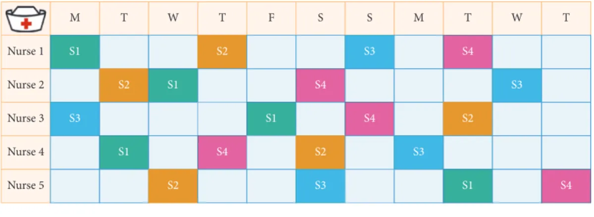
The NRP problem is a real-world problem at hospitals; the problem is to assign a predefined set of shifts (like S1-day shift, S2-noon shift, S3-night shift, and S4-Free-shift) of a scheduled period for a set of nurses of different preferences and skills in each ward. Figure 1 shows the illustrative example of the feasible nurse roster, which consists of four shifts, namely, day shift, noon shift, night shift, and free shift (holiday), allocating five nurses over 11 days of scheduled period. Each column in the scheduled table represents the day and the cell content represents the shift type allocated to a nurse. Each nurse is allocated one shift per day and the number of shifts is assigned based on the hospital contracts. This problem will have some variants on a number of shift types, nurses, nurse skills, contracts, and scheduling period. In general, both hard and soft constraints are considered for generating and assessing solutions.

Hard constraints are the regulations which must be satisfied to achieve the feasible solution. They cannot be violated since hard constraints are demanded by hospital regulations. The hard constraints HC1 to HC5 must be filled to schedule the roster. The soft constraints SC1 to SC14 are desirable, and the selection of soft constraints determines the quality of the roster. Tables 1 and 2 list the set of hard and soft constraints considered to solve the NRP. This section describes the mathematical model required for hard and soft constraints extensively.

The NRP consists of a set of nurses𝑛 = 1, 2, . . . , 𝑁, where

each row is specific to particular set of shifts𝑠 = 1, 2, . . . , 𝑆,

for the given set day𝑑 = 1, 2, . . . , 𝐷. The solution rosterS¸for

the0/1matrix dimension𝑁 ∗ 𝑆𝐷is as in

S¸_{𝑛,𝑑,𝑠}={_{

{

1 if nurse𝑛works𝑠shift for day𝑑

0 otherwise.

(1)

HC1. In this constraint, all demanded shifts are assigned to a

nurse.

𝑁

∑

𝑛=1

M T W T F Nurse 1 S1 S2 Nurse 2 S2 S1 Nurse 3 S3 S1 Nurse 4 S1 S4 Nurse 5 S2 S S M T W T S3 S4 S4 S3 S4 S2 S2 S3 S3 S1 S4 S2 S3 S4 S1 Day shift Noon shift Night shift Free shift

Figure 1: Illustrative example of Nurse Rostering Problem. Table 1

Hard constraints HC1 All demanded shifts assigned to a nurse. HC2 A nurse can work with only a single shift per day. HC3 The minimum number of nurses required for the shift.

HC4 The total number of working days for the nurse should be between the maximum and minimum range. HC5 A day shift followed by night shift is not allowed.

Table 2 Soft constraints

SC1 The maximum number of shifts assigned to each nurse. SC2 The minimum number of shifts assigned to each nurse.

SC3 The maximum number of consecutive working days assigned to each nurse. SC4 The minimum number of consecutive working days assigned to each nurse.

SC5 The maximum number of consecutive working days assigned to each nurse on which no shift is allotted. SC6 The minimum number of consecutive working days assigned to each nurse on which no shift is allotted. SC7 The maximum number of consecutive working weekends with at least one shift assigned to each nurse. SC8 The minimum number of consecutive working weekends with at least one shift assigned to each nurse. SC9 The maximum number of weekends with at least one shift assigned to each nurse.

SC10 Specific working day.

SC11 Requested day off.

SC12 Specific shift on.

SC13 Specific shift off.

SC14 Nurse not working on the unwanted pattern.

where𝐸_𝑑𝑠is the number of nurses required for a day(𝑑)at

shift (𝑠)and S¸_𝑑,𝑠 is the allocation of nurses in the feasible

solution roster.

HC2. In this constraint, each nurse can work not more than

one shift per day:

𝑆

∑

𝑠=1

S¸𝑠_𝑛,𝑑≤ 1, ∀𝑛 ∈ 𝑁, 𝑑 ∈ 𝐷, (3)

whereS¸_𝑛,𝑑is the allocation of nurses(𝑛)in solution at shift(𝑠)

for a day(𝑑).

HC3. This constraint deals with a minimum number of nurses

required for each shift.

𝑁

∑

𝑛=1

where min𝑛_𝑑,𝑠is the minimum number of nurses required for

a shift(𝑠)on the day(𝑑).

HC4. In this constraint, the total number of working days for

each nurse should range between minimum and maximum range for the given scheduled period.

𝑊min ≤ 𝐷 ∑ 𝑑=1 𝑆 ∑ 𝑠=1 S¸𝑑,𝑠_𝑛 ≤ 𝑊_max, ∀𝑛 ∈ 𝑁. (5) The average working shift for nurse can be determined by using 𝑊avg= _𝑁1 ( 𝐷 ∑ 𝑑=1 𝑆 ∑ 𝑠=1 S¸𝑑,𝑠_𝑛 , ∀𝑛 ∈ 𝑁) , (6)

where 𝑊_min and 𝑊_max are the minimum and maximum

number of days in scheduled period and𝑊_avgis the average

working shift of the nurse.

HC5. In this constraint, shift 1 followed by shift 3 is not

allowed; that is, a day shift followed by a night shift is not allowed. 𝑁 ∑ 𝑛=1 𝐷 ∑ 𝑑=1 S¸𝑛,𝑑_𝑠3 +S¸𝑛,𝑑+1_𝑠1 ≤ 1, ∀𝑠 ∈ 𝑆. (7)

SC1. The maximum number of shifts assigned to each nurse

for the given scheduled period is as follows:

max(( 𝐷 ∑ 𝑑=1 𝑆 ∑ 𝑠=1 S¸𝑑,𝑠_𝑛 − Φ𝑢𝑏_𝑛 ) , 0) , ∀𝑛 ∈ 𝑁, (8)

whereΦ𝑢𝑏_𝑛 is the maximum number of shifts assigned to nurse

(𝑛).

SC2. The minimum number of shifts assigned to each nurse

for the given scheduled period is as follows:

max((Φ𝑙𝑏_𝑛 − 𝐷 ∑ 𝑑=1 𝑆 ∑ 𝑠=1 S¸𝑑,𝑠_𝑛 ) , 0) , ∀𝑛 ∈ 𝑁, (9)

whereΦ𝑙𝑏_𝑛 is the minimum number of shifts assigned to nurse

(𝑛).

SC3. The maximum number of consecutive working days

assigned to each nurse on which a shift is allotted for the scheduled period is as follows:

Ψ𝑛

∑

𝑘=1

max((C𝑘_𝑛− Θ𝑢𝑏_𝑛 ) , 0) , ∀𝑛 ∈ 𝑁, (10)

whereΘ𝑢𝑏_𝑛 is the maximum number of consecutive working

days of nurse (𝑛), Ψ_𝑛 is the total number of consecutive

working spans of nurse(𝑛)in the roster, andC𝑘_𝑛is the count

of the𝑘th working spans of nurse(𝑛).

SC4. The minimum number of consecutive working days

assigned to each nurse on which a shift is allotted for the scheduled period is as follows:

Ψ𝑛

∑

𝑘=1

max((Θ𝑙𝑏_𝑛 −C𝑘_𝑛) , 0) , ∀𝑛 ∈ 𝑁, (11)

whereΘ𝑙𝑏_𝑛 is the minimum number of consecutive working

days of nurse (𝑛), Ψ_𝑛 is the total number of consecutive

working spans of nurse(𝑛)in the roster, andC𝑘_𝑛is the count

of the𝑘th working span of the nurse(𝑛).

SC5. The maximum number of consecutive working days

assigned to each nurse on which no shift is allotted for the given scheduled period is as follows:

Γ𝑛

∑

𝑘=1

max((ð𝑘_𝑛− 𝜑_𝑛𝑢𝑏) , 0) , ∀𝑛 ∈ 𝑁, (12)

where𝜑𝑢𝑏_𝑛 is the maximum number of consecutive free days of

nurse(𝑛),Γ_𝑛is the total number of consecutive free working

spans of nurse(𝑛)in the roster, andð𝑘_𝑛is the count of the𝑘th

working span of the nurse(𝑛).

SC6. The minimum number of consecutive working days

assigned to each nurse on which no shift is allotted for the given scheduled period is as follows:

Γ𝑛

∑

𝑘=1

max((𝜑𝑙𝑏_𝑛 − ð𝑘_𝑛) , 0) , ∀𝑛 ∈ 𝑁, (13)

where𝜑_𝑛𝑙𝑏is the minimum number of consecutive free days of

nurse(𝑛),Γ_𝑛is the total number of consecutive free working

spans of nurse(𝑛)in the roster, andð𝑘_𝑛is the count of the𝑘th

working span of the nurse(𝑛).

SC7. The maximum number of consecutive working

week-ends with at least one shift assigned to nurse for the given scheduled period is as follows:

̈Υ𝑛

∑

𝑘=1

max((𝜁_𝑛𝑘− Ω𝑢𝑏_𝑛 ) , 0) , ∀𝑛 ∈ 𝑁, (14)

whereΩ𝑢𝑏_𝑛 is the maximum number of consecutive working

weekends of nurse(𝑛), ̈Υ_𝑛is the total number of consecutive

working weekend spans of nurse(𝑛)in the roster, and𝜁_𝑛𝑘 is

the count of the𝑘th working weekend span of the nurse(𝑛).

SC8. The minimum number of consecutive working

week-ends with at least one shift assigned to nurse for the given scheduled period is as follows:

̈Υ𝑛

∑

𝑘=1

whereΩ𝑙𝑏_𝑛 is the minimum number of consecutive working

weekends of nurse(𝑛), ̈Υ_𝑛is the total number of consecutive

working weekend spans of nurse(𝑛)in the roster, and𝜁_𝑛𝑘 is

the count of the𝑘th working weekend span of the nurse(𝑛).

SC9. The maximum number of weekends with at least one

shift assigned to nurse in four weeks is as follows:

̈𝐼

𝑛

∑

𝑘=1

max((𝑘_𝑛− 𝜛𝑢𝑏_𝑛 ) , 0) , ∀𝑛 ∈ 𝑁, (16)

where𝑘_𝑛is the number of working days at the𝑘th weekend

of nurse(𝑛),𝜛𝑢𝑏_𝑛 is the maximum number of working days

for nurse(𝑛), and ̈𝐼_𝑛is the total count of the weekend in the

scheduling period of nurse(𝑛).

SC10. The nurse can request working on a particular day for

the given scheduled period.

𝐷

∑

𝑑=1

𝜆𝑑_𝑛= 1, ∀𝑛 ∈ 𝑁, (17)

where𝜆𝑑_𝑛is the day request from the nurse(𝑛)to work on any

shift on a particular day(𝑑).

SC11. The nurse can request that they do not work on a

particular day for the given scheduled period.

𝐷

∑

𝑑=1

𝜆𝑑_𝑛= 0, ∀𝑛 ∈ 𝑁, (18)

where𝜆𝑑_𝑛is the request from the nurse(𝑛)not to work on any

shift on a particular day(𝑑).

SC12. The nurse can request working on a particular shift on

a particular day for the given scheduled period.

𝐷 ∑ 𝑑=1 𝑆 ∑ 𝑠=1 Υ_𝑛𝑑,𝑠= 1, ∀𝑛 ∈ 𝑁, (19)

whereΥ_𝑛𝑑,𝑠is the shift request from the nurse(𝑛)to work on

a particular shift(𝑠)on particular day(𝑑).

SC13. The nurse can request that they do not work on a

particular shift on a particular day for the given scheduled period. 𝐷 ∑ 𝑑=1 𝑆 ∑ 𝑠=1Υ 𝑑,𝑠 𝑛 = 0, ∀𝑛 ∈ 𝑁, (20)

whereΥ_𝑛𝑑,𝑠is the shift request from the nurse(𝑛)not to work

on a particular shift(𝑠)on particular day(𝑑).

SC14. The nurse should not work on unwanted pattern

suggested for the scheduled period.

󰜚𝑛

∑

𝑢=1

𝜇𝑢_𝑛, ∀𝑛 ∈ 𝑁, (21)

where𝜇𝑢_𝑛is the total count of occurring patterns for nurse(𝑛)

of type𝑢;󰜚_𝑛is the set of unwanted patterns suggested for the

nurse(𝑛).

The objective function of the NRP is to maximize the nurse preferences and minimize the penalty cost from vio-lations of soft constraints in (22).

min𝑓 (S¸_{𝑛,𝑑,𝑠}) = ∑14 SC=1 𝑃sc( 𝑁 ∑ 𝑛=1 𝑆 ∑ 𝑠=1 𝐷 ∑ 𝑑=1 S¸_{𝑛,𝑑,𝑠}) ∗ 𝑇sc( 𝑁 ∑ 𝑛=1 𝑆 ∑ 𝑠=1 𝐷 ∑ 𝑑=1 S¸_{𝑛,𝑑,𝑠}) . (22)

Here SC refers to the set of soft constraints indexed in

Table 2,𝑃sc(𝑥)refers to the penalty weight violation of the

soft constraint, and𝑇sc(𝑥)refers to the total violations of the

soft constraints in roster solution. It has to be noted that the usage of penalty function [32] in the NRP is to improve the performance and provide the fair comparison with another optimization algorithm.

4. Bee Colony Optimization

4.1. Natural Behavior of Honey Bees. Swarm intelligence is an emerging discipline for the study of problems which requires an optimal approach rather than the traditional approach. The use of swarm intelligence is the part of artificial intelligence based on the study of the behavior of social insects. The swarm intelligence is composed of many individual actions using decentralized and self-organized system. Swarm behavior is characterized by natural behavior of many species such as fish schools, herds of animals, and flocks of birds formed for the biological requirements to stay together. Swarm implies the aggregation of animals such as birds, fishes, ants, and bees based on the collective behavior. The individual agents in the swarm will have a stochastic behavior which depends on the local perception of the neighborhood. The communication between any insects can be formed with the help of the colonies, and it promotes collective intelligence among the colonies.

The important features of swarms are proximity, quality, response variability, stability, and adaptability. The proximity of the swarm must be capable of providing simple space and time computations, and it should respond to the quality factors. The swarm should allow diverse activities and should not be restricted among narrow channels. The swarm should maintain the stability nature and should not fluctuate based on the behavior. The adaptability of the swarm must be able to change the behavior mode when required. Several hundreds of bees from the swarm work together to find nesting sites and select the best nest site. Bee Colony Optimization is inspired by the natural behavior of bees. The bee optimization algorithm is inspired by group decision-making processes of honey bees. A honey bee searches the best nest site by considering speed and accuracy.

In a bee colony there are three different types of bees, a single queen bee, thousands of male drone bees, and thousands of worker bees.

(1) The queen bee is responsible for creating new colonies by laying eggs.

(2) The male drone bees mated with the queen and were discarded from the colonies.

(3) The remaining female bees in the hive are called worker bees, and they are called the building block of the hive. The responsibilities of the worker bees are to feed, guard, and maintain the honey bee comb. Based on the responsibility, worker bees are classified as scout bees and forager bees. A scout bee flies in search of food sources randomly and returns when the energy gets exhausted. After reaching a hive scout bees share the information and start to explore rich food source locations with forager bees. The scout bee’s information includes direction, quality, quantity, and distance of the food source they found. The way of communicating information about a food source to foragers is done using dance. There are two types of dance, round dance and waggle dance. The round dance will provide direction of the food source when the distance is small. The waggle dance indicates the position and the direction of the food source; the distance can be measured by the speed of the dance. A greater speed indicates a smaller distance; and the quantity of the food depends on the wriggling of the bee. The exchange of information among hive mates is to acquire collective knowledge. Forager bees will silently observe the behavior of scout bee to acquire knowledge about the directions and information of the food source.

The group decision process of honey bees is for searching best food source and nest site. The decision-making process is based on the swarming process of the honey bee. Swarming is the process in which the queen bee and half of the worker bees will leave their hive to explore a new colony. The remaining worker bees and daughter bee will remain in the old hive to monitor the waggle dance. After leaving their parental hive, swarm bees will form a cluster in search of the new nest site. The waggle dance is used to communicate with quiescent bees, which are inactive in the colony. This provides precise information about the direction of the flower patch based on its quality and energy level. The number of follower bees increases based on the quality of the food source and allows the colony to gather food quickly and efficiently. The decision-making process can be done in two methods by swarm bees to find the best nest site. They are consensus and quorum; consensus is the group agreement taken into account and quorum is the decision process taken when the bee vote reaches a threshold value.

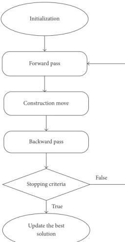
Bee Colony Optimization (BCO) algorithm is a population-based algorithm. The bees in the population are artificial bees, and each bee finds its neighboring solution from the current path. This algorithm has a forward and backward process. In forwarding pass, every bee starts to explore the neighborhood of its current solution and enables constructive and improving moves. In forward pass, entire bees in the hive will start the constructive move and then local search will start. In backward pass, bees share the objective value obtained in the forward pass. The bees with higher priority are used to discard all nonimproving moves. The bees will continue to explore in next forward pass or continue the same process with neighborhood. The flowchart

Forward pass Initialization

Construction move

Backward pass

Update the best solution Stopping criteria

False

True

Figure 2: Flowchart of BCO algorithm.

for BCO is shown in Figure 2. The BCO is proficient in solving combinatorial optimization problems by creating colonies of the multiagent system. The pseudocode for BCO is described in Algorithm 1. The bee colony system provides a standard well-organized and well-coordinated teamwork, multitasking performance [33].

4.2. Modified Nelder-Mead Method. The Nelder-Mead Method is a simplex method for finding a local minimum function of various variables and is a local search algorithm for unconstrained optimization problems. The whole search area is divided into different fragments and filled with bee agents. To obtain the best solution, each fragment can be searched by its bee agents through Modified Nelder-Mead Method (MNMM). Each agent in the fragments passes information about the optimized point using MNMM. By using NMMM, the best points are obtained, and the best solution is chosen by decision-making process of honey bees. The algorithm is a simplex-based method,

𝐷-dimensional simplex is initialized with 𝐷 + 1 vertices,

that is, two dimensions, and it forms a triangle; if it has three dimensions, it forms a tetrahedron. To assign the best and worst point, the vertices are evaluated and ordered based on the objective function.

The best point or vertex is considered to the minimum value of the objective function, and the worst point is chosen

Bee Colony Optimization

(1) Initialization: Assign every bee to an empty solution. (2) Forward Pass

For every bee (2.1) set𝑖 = 1;

(2.2) Evaluate all possible construction moves.

(2.3) Based on the evaluation, choose one move using Roulette Wheel. (2.4)𝑖 = 𝑖 + 1if (𝑖 ≤ 𝑁) Go to step (2.2)

where𝑖is the counter for construction move and𝑁is the number of construction moves during one forward pass.

(3) Return to Hive. (4) Backward Pass starts.

(5) Compute the objective function for each bee and sort accordingly.

(6) Calculate probability or logical reasoning to continue with the computed solution and become recruiter bee. (7) For every follower, choose the new solution from recruiters.

(8) If stopping criteria is not met Go to step (2). (9) Evaluate and find the best solution. (10) Output the best solution.

Algorithm 1: Pseudocode of BCO.

with a maximum value of the computed objective function. To form simplex new vertex function values are computed. This method can be calculated using four procedures, namely, reflection, expansion, contraction, and shrinkage. Figure 3 shows the operators of the simplex triangle in MNMM.

The simplex operations in each vertex are updated closer to its optimal solution; the vertices are ordered based on

fitness value and ordered. The best vertex is𝐴_𝑏, the second

best vertex is𝐴_𝑠, and the worst vertex is𝐴_𝑤calculated based

on the objective function. Let𝐴 = (𝑥, 𝑦)be the vertex in a

triangle as food source points;𝐴_𝑏 = (𝑥_𝑏, 𝑦_𝑏),𝐴_𝑠 = (𝑥_𝑠, 𝑦_𝑠)

and𝐴_𝑤= (𝑥_𝑤, 𝑦_𝑤)are the positions of the food source points,

that is, local optimal points. The objective functions for𝐴_𝑏,

𝐴_𝑠, and 𝐴_𝑤 are calculated based on (23) towards the food

source points.

The objective function to construct simplex to obtain local search using MNMM is formulated as

𝑓 (𝑥, 𝑦) = 𝑥2− 4𝑥 + 𝑦2− 𝑦 − 𝑥𝑦. (23) Based on the objective function value the vertices food points are ordered ascending with their corresponding honey

bee agents. The obtained values are ordered as𝐴_𝑏≤ 𝐴_𝑠≤ 𝐴_𝑤

with their honey bee position and food points in the simplex triangle. Figure 4 describes the search of best-minimized cost value for the nurse based on objective function (22). The working principle of Modified Nelder-Mead Method (MNMM) for searching food particles is explained in detail.

(1) In the simplex triangle the reflection coefficient 𝛼,

expansion coefficient𝛾, contraction coefficient𝛽, and

shrinkage coefficient𝛿are initialized.

(2) The objective function for the simplex triangle ver-tices is calculated and ordered. The best vertex with

lower objective value is𝐴_𝑏, the second best vertex is

𝐴_𝑠, and the worst vertex is named as𝐴_𝑤, and these

vertices are ordered based on the objective function

as𝐴_𝑏≤ 𝐴_𝑠≤ 𝐴_𝑤.

(3) The first two best vertices are selected, namely,𝐴_𝑏and

𝐴_𝑠, and the construction proceeds with calculating

the midpoint of the line segment which joins the two best vertices, that is, food positions. The objective function decreases as the honey agent associated with the worst position vertex moves towards best and second best vertices. The value decreases as the honey

agent moves towards𝐴_𝑤to𝐴_𝑏 and𝐴_𝑤 to𝐴_𝑠. It is

feasible to calculate the midpoint vertex𝐴_𝑚 by the

line joining best and second best vertices using

𝐴𝑚= 𝐴𝑏+ 𝐴₂ 𝑠. (24)

(4) A reflecting vertex𝐴_𝑟 is generated by choosing the

reflection of worst point𝐴_𝑤. The objective function

value for𝐴_𝑟 is𝑓(𝐴_𝑟) which is calculated, and it is

compared with worst vertex 𝐴_𝑤 objective function

value𝑓(𝐴_𝑤). If𝑓(𝐴_𝑟) < 𝑓(𝐴_𝑤)proceed with step

(5), the reflection vertex can be calculated using

𝐴_𝑟 = 𝐴_𝑚+ 𝛼 (𝐴_𝑚− 𝐴_𝑤) , where𝛼 > 0. (25) (5) The expansion process starts when the objective

function value at reflection vertex𝐴_𝑟 is lesser than

worst vertex 𝐴_𝑤, 𝑓(𝐴_𝑟) < 𝑓(𝐴_𝑤), and the line

segment is further extended to𝐴_𝑒 through𝐴_𝑟 and

𝐴_𝑤. The vertex point𝐴_𝑒 is calculated by (26). If the

objective function value at𝐴_𝑒is lesser than reflection

vertex𝐴_𝑟, 𝑓(𝐴_𝑒) < 𝑓(𝐴_𝑟), then the expansion is

accepted, and the honey bee agent has found best food position compared with reflection point.

𝐴_𝑒= 𝐴_𝑟+ 𝛾 (𝐴_𝑟− 𝐴_𝑚) , where𝛾 > 1. (26)

(6) The contraction process is carried out when𝑓(𝐴_𝑟) <

Aw

As

Ab

(a) Simplex triangle

Ar As Ab Aw (b) Reflection Ae Ar As Ab Aw (c) Expansion Ac As Ab Aw (d) Contraction (𝐴ℎ< 𝐴𝑟) Ac As Ab Aw (e) Contraction (𝐴𝑟< 𝐴ℎ) A㰀_b A㰀s As Ab Aw (f) Shrinkage

Figure 3: Nelder-Mead operations.

𝐴_𝑟. If 𝑓(𝐴_𝑟) > 𝑓(𝐴_ℎ) then the direct contraction

without the replacement of𝐴_𝑏with𝐴_𝑟is performed.

The contraction vertex𝐴_𝑐can be calculated using

𝐴𝑐 = 𝛽𝐴𝑟+ (1 − 𝛽) 𝐴𝑚, where0 < 𝛽 < 1. (27)

If𝑓(𝐴_𝑟) ≤ 𝑓(𝐴_𝑏), the contraction can be done and

𝐴_𝑐replaced with𝐴_ℎ; go to step (8) or else proceed to

step (7).

(7) The shrinkage phase proceeds when the contraction

process at step (6) fails and is done by shrinking all

the vertices of the simplex triangle except𝐴_ℎ using

(28). The objective function value of reflection and contraction phase is not lesser than the worst point;

then the vertices𝐴_𝑠and𝐴_𝑤must be shrunk towards

𝐴_ℎ.Thus the vertices of smaller value will form a new

simplex triangle with another two best vertices.

𝐴_𝑖= 𝛿𝐴_𝑖+ 𝐴₁(1 − 𝛿) , where0 < 𝛿 < 1. (28)

(8) The calculations are stopped when the termination condition is met.

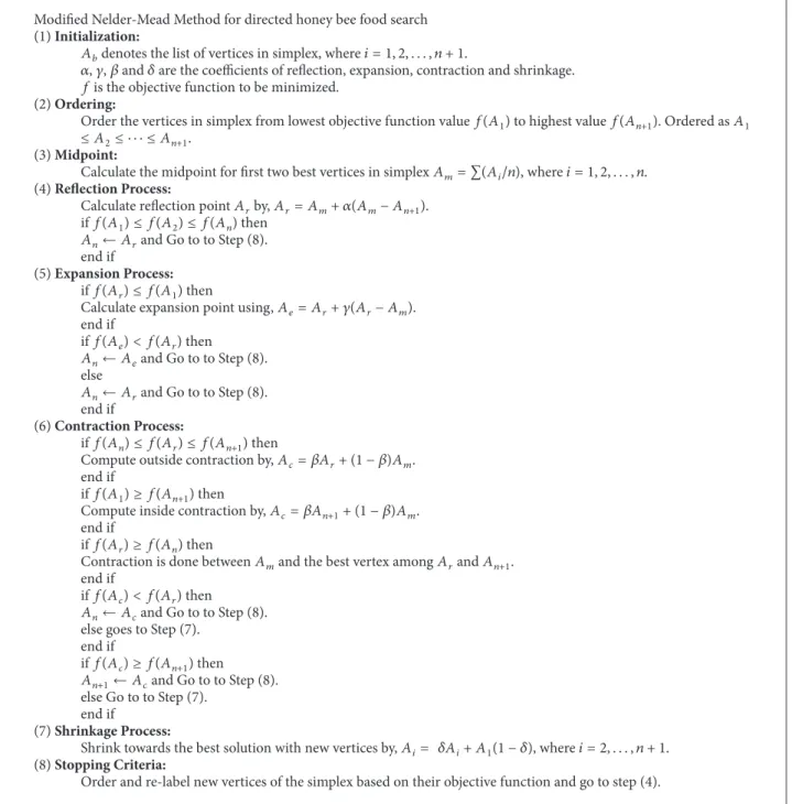
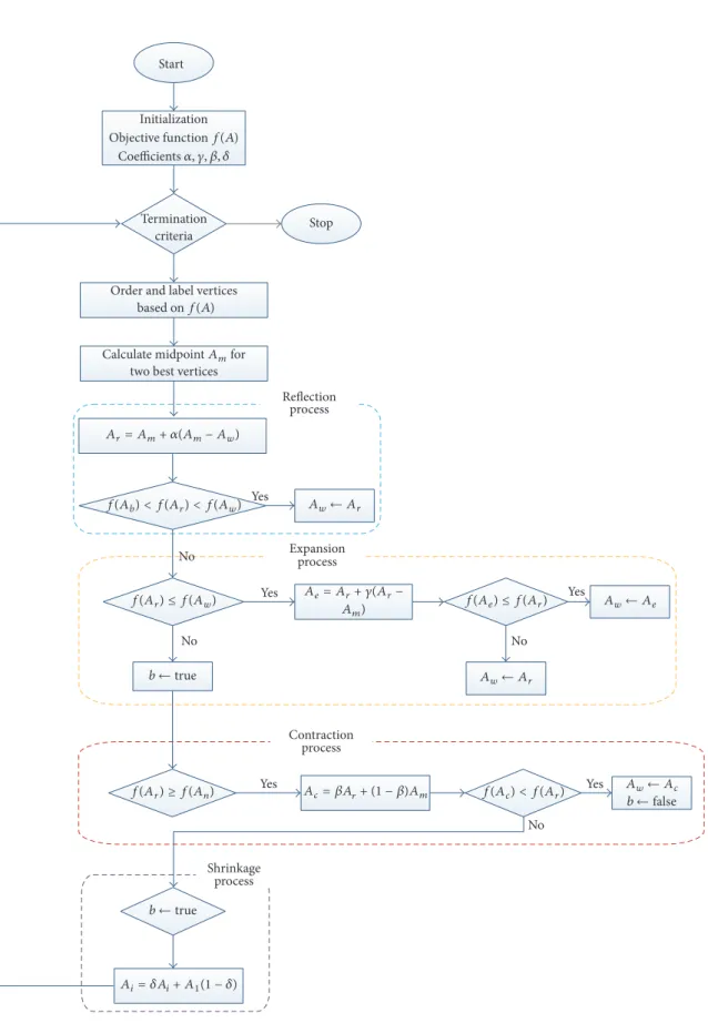
Algorithm 2 describes the pseudocode for Modified Nelder-Mead Method in detail. It portraits the detailed pro-cess of MNMM to obtain the best solution for the NRP. The workflow of the proposed MNMM is explained in Figure 5.

5. MODBCO

Bee Colony Optimization is the metaheuristic algorithm to solve various combinatorial optimization problems, and it is inspired by the natural behavior of bee for their food sources. The algorithm consists of two steps, forward and backward pass. During forwarding pass, bees started to explore the neighborhood of its current solution and find all possible ways. In backward pass, bees return to the hive and share the values of the objective function of their current solution. Calculate nectar amount using probability

Ab Aw Ar As Am d d Ab Aw Ar As Am d d Ae d/2 Ab Aw Ar As Am Ac1 Ac2 Ab Aw As Am Anew

Figure 4: Bees search movement based on MNMM.

function and advertise the solution; the bee which has the better solution is given higher priority. The remaining bees based on the probability value decide whether to explore the solution or proceed with the advertised solution. Directed Bee Colony Optimization is the computational system where several bees work together in uniting and interact with each other to achieve goals based on the group decision process. The whole search area of the bee is divided into multiple fragments; different bees are sent to different fragments. The best solution in each fragment is obtained by using a local search algorithm Modified Nelder-Mead Method (MNMM). To obtain the best solution, the total varieties of individual parameters are partitioned into individual volumes. Each volume determines the starting point of the exploration of food particle by each bee. The bees use developed MNMM algorithm to find the best solution by remembering the last two best food sites they obtained. After obtaining the current solution, the bee starts to backward pass, sharing of information obtained during forwarding pass. The bees started to share information about optimized point by the natural behavior of bees called waggle dance. When all the information about the best food is shared, the best among the optimized point is chosen using a decision-making process called consensus and quorum method in honey bees [34, 35].

5.1. Multiagent System. All agents live in an environment which is well structured and organized. In multiagent system, several agents work together and interact with each other to obtain the goal. According to Jiao and Shi [36] and Zhong et al. [37] all agents should possess the following qualities: agents should live and act in an environment, each agent should sense its local environment, each agent

should be capable of interacting with other agents in a local environment, and agents attempt to perform their goal. All agents interact with each other and take the decision to achieve the desired goals. The multiagent system is a com-putational system and provides an opportunity to optimize and compute all complex problems. In multiagent system, all agents start to live and act in the same environment which is well organized and structured. Each agent in the environment is fixed on a lattice point. The size and dimension of the lattice point in the environment depend upon the variables used. The objective function can be calculated based on the parameters fixed.

(1) Consider “𝑒” number of independent parameters to

calculate the objective function. The range of the𝑔th

parameter can be calculated using [𝑄_𝑔𝑖, 𝑄_𝑔𝑓], where

𝑄_𝑔𝑖 is the initial value of the𝑔th parameter and𝑄_𝑔𝑓

is the final value of the𝑔th parameter chosen.

(2) Thus the objective function can be formulated as𝑒

number of axes; each axis will contain a total range of single parameter with different dimensions. (3) Each axis is divided into smaller parts; each part

is called a step. So𝑔th axis can be divided into 𝑛_𝑔

number of steps each with the length of𝐿_𝑔, where the

value of𝑔depends upon parameters; thus𝑔 = 1to𝑒.

The relationship between𝑛_𝑔and𝐿_𝑔can be given as

𝑛_𝑔=𝑄𝑔𝑖− 𝑄𝑔𝑓

𝐿𝑔 . (29)

(4) Then each axis is divided into branches, for

Modified Nelder-Mead Method for directed honey bee food search

(1)Initialization:

𝐴𝑏denotes the list of vertices in simplex, where𝑖 = 1, 2, . . . , 𝑛 + 1.

𝛼,𝛾,𝛽and𝛿are the coefficients of reflection, expansion, contraction and shrinkage.

𝑓is the objective function to be minimized.

(2)Ordering:

Order the vertices in simplex from lowest objective function value𝑓(𝐴₁) to highest value𝑓(𝐴_𝑛+1). Ordered as𝐴₁

≤ 𝐴2≤ ⋅ ⋅ ⋅ ≤ 𝐴𝑛+1.

(3)Midpoint:

Calculate the midpoint for first two best vertices in simplex𝐴_𝑚= ∑(𝐴_𝑖/𝑛), where𝑖 = 1, 2, . . . , 𝑛.

(4)Reflection Process:

Calculate reflection point𝐴_𝑟by,𝐴_𝑟= 𝐴_𝑚+ 𝛼(𝐴_𝑚− 𝐴_𝑛+1). if𝑓(𝐴₁) ≤ 𝑓(𝐴₂) ≤ 𝑓(𝐴_𝑛)then

𝐴_𝑛← 𝐴_𝑟and Go to to Step (8). end if

(5)Expansion Process:

if𝑓(𝐴_𝑟) ≤ 𝑓(𝐴₁) then

Calculate expansion point using,𝐴_𝑒= 𝐴_𝑟+ 𝛾(𝐴_𝑟− 𝐴_𝑚). end if if𝑓(𝐴_𝑒) < 𝑓(𝐴_𝑟) then 𝐴𝑛← 𝐴𝑒and Go to to Step (8). else 𝐴𝑛← 𝐴𝑟and Go to to Step (8). end if (6)Contraction Process: if𝑓(𝐴_𝑛) ≤ 𝑓(𝐴_𝑟) ≤ 𝑓(𝐴_𝑛+1)then

Compute outside contraction by,𝐴_𝑐= 𝛽𝐴_𝑟+ (1 − 𝛽)𝐴_𝑚. end if

if𝑓(𝐴₁) ≥ 𝑓(𝐴_𝑛+1) then

Compute inside contraction by,𝐴_𝑐= 𝛽𝐴_𝑛+1+ (1 − 𝛽)𝐴_𝑚. end if

if𝑓(𝐴_𝑟) ≥ 𝑓(𝐴_𝑛) then

Contraction is done between𝐴_𝑚and the best vertex among𝐴_𝑟and𝐴_𝑛+1. end if

if𝑓(𝐴_𝑐) < 𝑓(𝐴_𝑟) then

𝐴𝑛← 𝐴𝑐and Go to to Step (8).

else goes to Step (7). end if if𝑓(𝐴_𝑐) ≥ 𝑓(𝐴_𝑛+1) then 𝐴_𝑛+1← 𝐴_𝑐and Go to to Step (8). else Go to to Step (7). end if (7)Shrinkage Process:

Shrink towards the best solution with new vertices by,𝐴_𝑖= 𝛿𝐴_𝑖+ 𝐴₁(1 − 𝛿), where𝑖 = 2, . . . , 𝑛 + 1.

(8)Stopping Criteria:

Order and re-label new vertices of the simplex based on their objective function and go to step (4).

Algorithm 2: Pseudocode of Modified Nelder-Mead Method.

𝑒-dimensional volume. Total number of volumes𝑁_V

can be formulated using

𝑁_V=∏𝑒

𝑔=1𝑛𝑔. (30)

(5) The starting point of the agent in the environment, which is one point inside volume, is chosen by calculating the midpoint of the volume. The midpoint of the lattice can be calculated as

[𝑄𝑖1− 𝑄𝑓1 2 , 𝑄_𝑖2− 𝑄_𝑓2 2 , . . . , 𝑄_𝑖𝑒− 𝑄_𝑓𝑒 2 ] . (31)

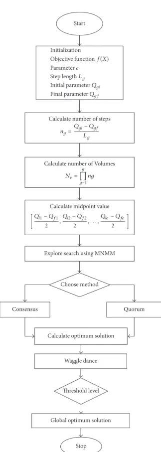
5.2. Decision-Making Process. A key role of the honey bees is to select the best nest site and is done by the process of decision-making to produce a unified decision. They follow a distributed decision-making process to find out the neighbor nest site for their food particles. The pseudocode for the proposed MODBCO algorithm is shown in Algorithm 3. Figure 6 explains the workflow of the proposed algorithm for the search of food particles by honey bees using MODBCO. 5.2.1. Waggle Dance. The scout bees after returning from the search of food particle report about the quality of the food site by communication mode called waggle dance. Scout bees perform the waggle dance to other quiescent bees to advertise

Yes

Reflection process Order and label vertices

based onf(A) Initialization Coefficients훼, 훾, 훽, 훿

Objective functionf(A)

f(Ab) < f(Ar) < f(Aw) Aw← Ar

f(Ae) ≤ f(Ar)

two best vertices

Amfor Calculate midpoint Start Termination criteria Stop Ar= Am+ 훼(Am− Aw) Expansion process No Yes f(Ar) ≤ f(Aw) Aw← Ae No b ←true Aw← Ar Contraction process f(Ar) ≥ f(An) Yes f(Ac) < f(Ar) Aw← Ac b ←false No Shrinkage process b ←true Yes Yes No Ae= Ar+ 훾(Ar− Am) Ac= 훽Ar+ (1 − 훽)Am Ai= 훿Ai+ A1(1 − 훿)

Multi-Objective Directed Bee Colony Optimization (1) Initialization:

𝑓(𝑥)is the objective function to be minimized.

Initialize𝑒number of parameters and𝐿_𝑔length of steps where𝑔 = 0to𝑒. Initialize initial value and the final value of the parameter as𝑄_𝑔𝑖and𝑄_𝑔𝑓.

/∗∗_{Solution Representation}∗∗_/

The solutions are represented in the form of Binary values, which can be generated as follows For each solution𝑖 = 1:𝑛

𝑋_𝑖= {𝑥_𝑖,1, 𝑥_𝑖,2, . . . , 𝑥_𝑖,𝑑| 𝑑 ∈total days &𝑥_𝑖,𝑑=rand≥ 0.29 ∀𝑑} End for

(2) The number of steps in each step can be calculated using

𝑛_𝑔= 𝑄𝑔𝑖− 𝑄𝑔𝑓 𝐿𝑔

(3) The total number of volumes can be calculated using

𝑁V = 𝑒

∏

𝑔=1𝑛𝑔

(4) The midpoint of the volume to calculate starting point of the exploration can be calculated using

[𝑄𝑖1− 𝑄𝑓1 2 , 𝑄𝑖2− 𝑄𝑓2 2 , . . . , 𝑄𝑖𝑒− 𝑄𝑓𝑒 2 ]

(5) Explore the search volume according to the Modified Nelder-Mead Method using Algorithm 2. (6) The recorded value of the optimized point in vector table using

[𝑓(𝑉1), 𝑓(𝑉2), . . . , 𝑓(𝑉𝑁V)]

(7) The globally optimized point is chosen based on Bee decision-making process using Consensus and Quorum method approach

𝑓(𝑉𝑔) =min[𝑓(𝑉1) , 𝑓(𝑉2), . . . , 𝑓(𝑉𝑁V)]

Algorithm 3: Pseudocode of MODBCO.

their best nest site for the exploration of food source. In the multiagent system, each agent after collecting individual solution gives it to the centralized systems. To select the best optimal solution for minimal optimal cases, the mathematical formulation can be stated as

dance_𝑖=min(𝑓_𝑖(𝑉)) . (32)

This mathematical formulation will find the minimal

optimal cases among the search solution, where𝑓_𝑖(𝑉)is the

search value calculated by the agent. The search values are

recorded in the vector table𝑉;𝑉is the vector which consists

of𝑒number of elements. The element𝑒contains the value of

the parameter; both optimal solution and parameter values are recorded in the vector table.

5.2.2. Consensus. The consensus is the widespread agreement among the group based on voting; the voting pattern of the scout bees is monitored periodically to know whether it reached an agreement and started acting on the decision pattern. Honey bees use the consensus method to select the best search value; the globally optimized point is chosen by comparing the values in the vector table. The globally opti-mized points are selected using the mathematical formulation

𝑓 (𝑉_𝑔) =min[𝑓 (𝑉₁) , 𝑓 (𝑉₂) , . . . , 𝑓 (𝑉_𝑁V)] . (33) 5.2.3. Quorum. In quorum method, the optimum solution is calculated as the final solution based on the threshold level obtained by the group decision-making process. When the

solution reaches the optimal threshold level𝜉_𝑞, then the

solu-tion is considered as a final solusolu-tion based on unison decision process. The quorum threshold value describes the quality of

the food particle result. When the threshold value is less the computation time decreases, but it leads to inaccurate experi-mental results. The threshold value should be chosen to attain less computational time with an accurate experimental result.

6. Experimental Design and Analysis

6.1. Performance Metrics. The performance of the proposed algorithm MODBCO is assessed by comparing with five different competitor methods. Here six performance metrics are considered to investigate the significance and evaluate the experimental results. The metrics are listed in this section. 6.1.1. Least Error Rate. Least Error Rate (LER) is the percent-age of the difference between known optimal value and the best value obtained. The LER can be calculated using

LER(%) =

𝑟

∑

𝑖=1

Optimal_NRP-Instance−fitness𝑖

Optimal_NRP-Instance . (34)

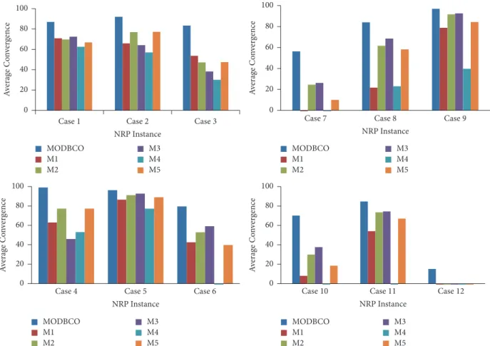
6.1.2. Average Convergence. The Average Convergence is the measure to evaluate the quality of the generated population on average. The Average Convergence (AC) is the percentage of the average of the convergence rate of solutions. The per-formance of the convergence time is increased by the Average Convergence to explore more solutions in the population. The Average Convergence is calculated using

AC

=∑𝑟

𝑖=1

1 −Avg_fitness𝑖−OptimalNRP-Instance

Optimal_NRP-Instance ∗ 100,

(35)

Start

Choose method Explore search using MNMM

Consensus Quorum

Calculate optimum solution

Waggle dance

Threshold level

Global optimum solution

Stop Calculate number of steps

ng=

Qgi− Qgf

Lg

Calculate midpoint value

[Qi1− Qf1 2 , Qi2− Qf2 2 , . . . , Qie− Qfe 2 ]

Calculate number of Volumes

N= g ∏ g−1 ng Initialization Parameter e Objective functionf(X) Lg Step length Qgi Initial parameter Qgf Final parameter

6.1.3. Standard Deviation. Standard deviation (SD) is the measure of dispersion of a set of values from its mean value. Average Standard Deviation is the average of the

standard deviation of all instances taken from the dataset. The Average Standard Deviation (ASD) can be calculated using

ASD= √

𝑟

∑

𝑖=1

(value obtained in each instance_𝑖−Mean value of the instance)2, (36)

where(𝑟)is the number of instances in the given dataset.

6.1.4. Convergence Diversity. The Convergence Diversity (CD) is the difference between best convergence rate and worst convergence rate generated in the population. The Convergence Diversity can be calculated using

CD=Convergence_best−Convergence_worst, (37)

where Convergence_bestis the convergence rate of best fitness

individual and Convergence_worst is the convergence rate of

worst fitness individual in the population.

6.1.5. Cost Diversion. Cost reduction is the difference between known cost in the NRP Instances and the cost obtained from our approach. Average Cost Diversion (ACD) is the average of cost diversion to the total number of instan-ces taken from the dataset. The value of ACR can be calculated from

ACR=

𝑟

∑

𝑖=1

Cost_𝑖−CostNRP-Instance

Total number of instances, (38)

where(𝑟)is the number of instances in the given dataset.

6.2. Experimental Environment Setup. The proposed Direct-ed Bee Colony algorithm with the ModifiDirect-ed Nelder-Mead Method to solve the NRP is illustrated briefly in this section. The main objective of the proposed algorithm is to satisfy multiobjective of the NRP as follows:

(a) Minimize the total cost of the rostering problem. (b) Satisfy all the hard constraints described in Table 1.

(c) Satisfy as many soft constraints described in Table 2. (d) Enhance the resource utilization.

(e) Equally distribute workload among the nurses. The Nurse Rostering Problem datasets are taken from the First International Rostering Competition (INRC2010) by PATAT-2010, a leading conference in Automated Timetabling [38]. The INRC2010 dataset is divided based on its complexity and size into three tracks, namely, sprint, medium, and long datasets. Each track is divided into four types as early, late, hidden, and hint with reference to the competition INRC2010. The first track sprint is the easiest and consists of 10 nurses, 33 datasets which are sorted as 10 early types, 10 late types, 10 hidden types, and 3 hint type datasets. The scheduling period is for 28 days with 3 to 4 contract types, 3 to 4 daily shifts, and one skill specification. The second track

is a medium which is more complex than sprint track, and it consists of 30 to 31 nurses, 18 datasets which are sorted as 5 early types, 5 long types, 5 hidden types, and 3 hint types. The scheduling period is for 28 days with 3 to 4 contract types, 4 to 5 daily shifts, and 1 to 2 skill specifications. The most complicated track is long with 49 to 40 nurses and consists of 18 datasets which are sorted as 5 early types, 5 long types, 5 hidden types, and 3 hint types. The scheduling period for this track is 28 days with 3 to 4 contract types, 5 daily shifts, and 2 skill specifications. The detailed description of the datasets available in the INRC2010 is shown in Table 3. The datasets are classified into twelve cases based on the size of the instances and listed in Table 4.

Table 3 describes the detailed description of the datasets; columns one to three are used to index the dataset to track, type, and instance. Columns four to seven will explain the number of available nurses, skill specifications, daily shift types, and contracts. Column eight explains the number of unwanted shift patterns in the roster. The nurse preferences are managed by shift off and day off in columns nine and ten. The number of weekend days is shown in column eleven. The

last column indicates the scheduling period. The symbol “𝑥”

shows there is no shift off and day off with the corresponding datasets.

Table 4 shows the list of datasets used in the experiment, and it is classified based on its size. The datasets present

in case1 to case4are smaller in size, case 5to case 8are

considered to be medium in size, and the larger sized dataset

is classified from case9to case12.

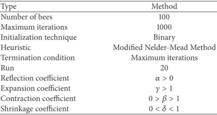
The performance of MODBCO for NRP is evaluated using INRC2010 dataset. The experiments are done on dif-ferent optimization algorithms under similar environment conditions to assess the performance. The proposed algo-rithm to solve the NRP is coded using MATLAB 2012 platform under Windows on an Intel 2 GHz Core 2 quad processor with 2 GB of RAM. Table 3 describes the instances considered by MODBCO to solve the NRP. The empirical evaluations will set the parameters of the proposed system. Appropriate parameter values are determined based on the preliminary experiments. The list of competitor methods chosen to evaluate the performance of the proposed algo-rithm is shown in Table 5. The heuristic parameter and the corresponding values are represented in Table 6.

6.3. Statistical Analysis. Statistical analysis plays a major role in demonstrating the performance of the proposed algorithm over existing algorithms. Various statistical tests and measures to validate the performance of the algorithm are reviewed by Demˇsar [39]. The authors used statistical tests

Table 3: The features of the INRC2010 datasets.

Track Type Instance Nurses Skills Shifts Contracts Unwanted pattern Shift off Day off Weekend Time period

Sprint Early 01–10 10 1 4 4 3 ✓ ✓ 2 1-01-2010 to 28-01-2010 Hidden 01-02 10 1 3 3 4 ✓ ✓ 2 1-06-2010 to 28-06-2010 03, 05, 08 10 1 4 3 8 ✓ ✓ 2 1-06-2010 to 28-06-2010 04, 09 10 1 4 3 8 ✓ ✓ 2 1-06-2010 to 28-06-2010 06, 07 10 1 3 3 4 ✓ ✓ 2 1-01-2010 to 28-01-2010 10 10 1 4 3 8 ✓ ✓ 2 1-01-2010 to 28-01-2010 Late 01, 03–05 10 1 4 3 8 ✓ ✓ 2 1-01-2010 to 28-01-2010 02 10 1 3 3 4 ✓ ✓ 2 1-01-2010 to 28-01-2010 06, 07, 10 10 1 4 3 0 ✓ ✓ 2 1-01-2010 to 28-01-2010 08 10 1 4 3 0 × × 2 1-01-2010 to 28-01-2010 09 10 1 4 3 0 × × 2, 3 1-01-2010 to 28-01-2010 Hint 01, 03 10 1 4 3 8 ✓ ✓ 2 1-01-2010 to 28-01-2010 02 10 1 4 3 0 ✓ ✓ 2 1-01-2010 to 28-01-2010 Medium Early 01–05 31 1 4 4 0 ✓ ✓ 2 1-01-2010 to 28-01-2010 Hidden 01–04 30 2 5 4 9 × × 2 1-06-2010 to 28-06-2010 05 30 2 5 4 9 × × 2 1-06-2010 to 28-06-2010 Late 01 30 1 4 4 7 ✓ ✓ 2 1-01-2010 to 28-01-2010 02, 04 30 1 4 3 7 ✓ ✓ 2 1-01-2010 to 28-01-2010 03 30 1 4 4 0 ✓ ✓ 2 1-01-2010 to 28-01-2010 05 30 2 5 4 7 ✓ ✓ 2 1-01-2010 to 28-01-2010 Hint 01, 03 30 1 4 4 7 ✓ ✓ 2 1-01-2010 to 28-01-2010 02 30 1 4 4 7 ✓ ✓ 2 1-01-2010 to 28-01-2010 Long Early 01–05 49 2 5 3 3 ✓ ✓ 2 1-01-2010 to 28-01-2010 Hidden 01–04 50 2 5 3 9 × × 2, 3 1-06-2010 to 28-06-2010 05 50 2 5 3 9 × × 2, 3 1-06-2010 to 28-06-2010 Late 01, 03, 05 50 2 5 3 9 × × 2, 3 1-01-2010 to 28-01-2010 02, 04 50 2 5 4 9 × × 2, 3 1-01-2010 to 28-01-2010 Hint 01 50 2 5 3 9 × × 2, 3 1-01-2010 to 28-01-2010 02, 03 50 2 5 3 7 × × 2 1-01-2010 to 28-01-2010

Table 4: Classification of INRC2010 datasets based on the size.

SI number Case Track Type

1 Case1 Sprint Early

2 Case2 Sprint Hidden

3 Case3 Sprint Late

4 Case4 Sprint Hint

5 Case5 Middle Early

6 Case6 Middle Hidden

7 Case7 Middle Late

8 Case8 Middle Hint

9 Case9 Long Early

10 Case10 Long Hidden

11 Case11 Long Late

12 Case12 Long Hint

like ANOVA, Dunnett test, and post hoc test to substantiate the effectiveness of the proposed algorithm and help to differentiate from existing algorithms.

6.3.1. ANOVA Test. To validate the performance of the proposed algorithm, ANOVA (Analysis of Variance) is used as the statistical analysis tool to demonstrate whether one or more solutions significantly vary [40]. The authors used one-way ANOVA test [41] to show significance in proposed algorithm. One-way ANOVA is used to validate and compare

Table 5: List of competitors methods to compare.

Type Method Reference

M₁ Artificial Bee Colony Algorithm [14] M₂ Hybrid Artificial Bee Colony Algorithm [15]

M₃ Global best harmony search [16]

M₄ Harmony Search with Hill Climbing [17] M₅ Integer Programming Technique for NRP [18] Table 6: Configuration parameter for experimental evaluation.

Type Method

Number of bees 100

Maximum iterations 1000

Initialization technique Binary

Heuristic Modified Nelder-Mead Method

Termination condition Maximum iterations

Run 20

Reflection coefficient 𝛼 > 0 Expansion coefficient 𝛾 > 1 Contraction coefficient 0 > 𝛽 > 1 Shrinkage coefficient 0 < 𝛿 < 1

differences between various algorithms. The ANOVA test is performed with 95% confidence interval, the significant level of 0.05. In ANOVA test, the null hypothesis is tested to show the difference in the performance of the algorithms.

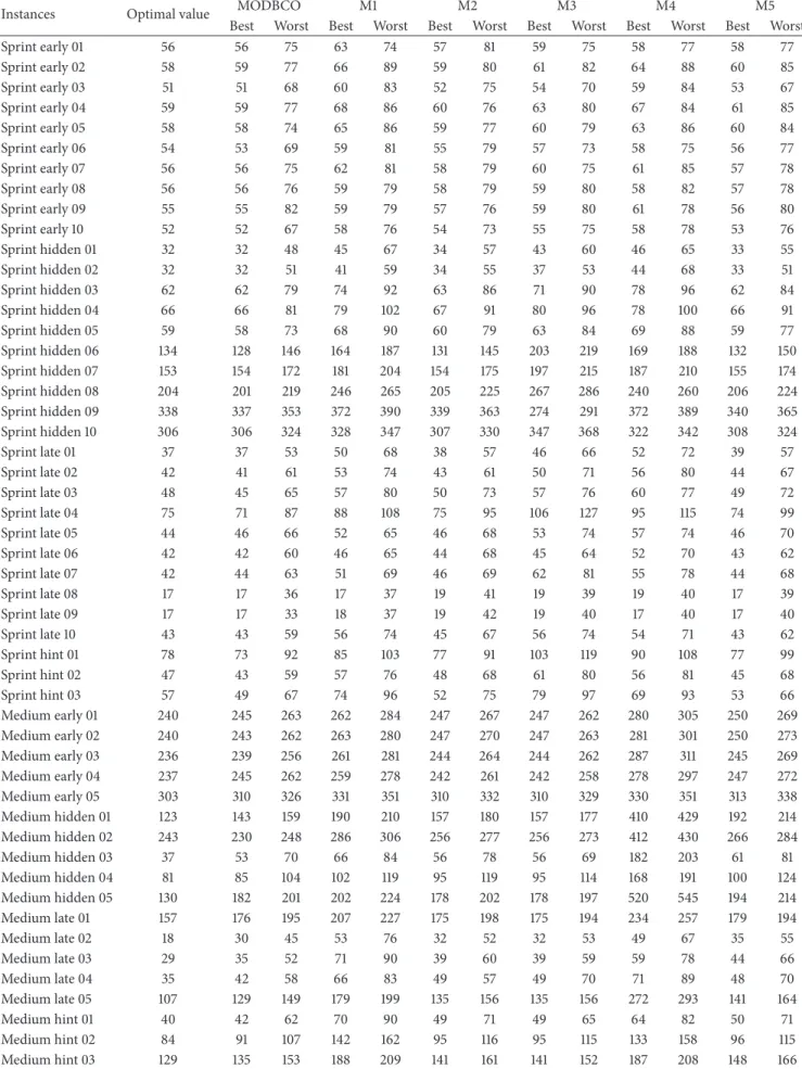
Table 7: Experimental result with respect to best value.

Instances Optimal value MODBCO M1 M2 M3 M4 M5

Best Worst Best Worst Best Worst Best Worst Best Worst Best Worst

Sprint early 01 56 56 75 63 74 57 81 59 75 58 77 58 77 Sprint early 02 58 59 77 66 89 59 80 61 82 64 88 60 85 Sprint early 03 51 51 68 60 83 52 75 54 70 59 84 53 67 Sprint early 04 59 59 77 68 86 60 76 63 80 67 84 61 85 Sprint early 05 58 58 74 65 86 59 77 60 79 63 86 60 84 Sprint early 06 54 53 69 59 81 55 79 57 73 58 75 56 77 Sprint early 07 56 56 75 62 81 58 79 60 75 61 85 57 78 Sprint early 08 56 56 76 59 79 58 79 59 80 58 82 57 78 Sprint early 09 55 55 82 59 79 57 76 59 80 61 78 56 80 Sprint early 10 52 52 67 58 76 54 73 55 75 58 78 53 76 Sprint hidden 01 32 32 48 45 67 34 57 43 60 46 65 33 55 Sprint hidden 02 32 32 51 41 59 34 55 37 53 44 68 33 51 Sprint hidden 03 62 62 79 74 92 63 86 71 90 78 96 62 84 Sprint hidden 04 66 66 81 79 102 67 91 80 96 78 100 66 91 Sprint hidden 05 59 58 73 68 90 60 79 63 84 69 88 59 77 Sprint hidden 06 134 128 146 164 187 131 145 203 219 169 188 132 150 Sprint hidden 07 153 154 172 181 204 154 175 197 215 187 210 155 174 Sprint hidden 08 204 201 219 246 265 205 225 267 286 240 260 206 224 Sprint hidden 09 338 337 353 372 390 339 363 274 291 372 389 340 365 Sprint hidden 10 306 306 324 328 347 307 330 347 368 322 342 308 324 Sprint late 01 37 37 53 50 68 38 57 46 66 52 72 39 57 Sprint late 02 42 41 61 53 74 43 61 50 71 56 80 44 67 Sprint late 03 48 45 65 57 80 50 73 57 76 60 77 49 72 Sprint late 04 75 71 87 88 108 75 95 106 127 95 115 74 99 Sprint late 05 44 46 66 52 65 46 68 53 74 57 74 46 70 Sprint late 06 42 42 60 46 65 44 68 45 64 52 70 43 62 Sprint late 07 42 44 63 51 69 46 69 62 81 55 78 44 68 Sprint late 08 17 17 36 17 37 19 41 19 39 19 40 17 39 Sprint late 09 17 17 33 18 37 19 42 19 40 17 40 17 40 Sprint late 10 43 43 59 56 74 45 67 56 74 54 71 43 62 Sprint hint 01 78 73 92 85 103 77 91 103 119 90 108 77 99 Sprint hint 02 47 43 59 57 76 48 68 61 80 56 81 45 68 Sprint hint 03 57 49 67 74 96 52 75 79 97 69 93 53 66 Medium early 01 240 245 263 262 284 247 267 247 262 280 305 250 269 Medium early 02 240 243 262 263 280 247 270 247 263 281 301 250 273 Medium early 03 236 239 256 261 281 244 264 244 262 287 311 245 269 Medium early 04 237 245 262 259 278 242 261 242 258 278 297 247 272 Medium early 05 303 310 326 331 351 310 332 310 329 330 351 313 338 Medium hidden 01 123 143 159 190 210 157 180 157 177 410 429 192 214 Medium hidden 02 243 230 248 286 306 256 277 256 273 412 430 266 284 Medium hidden 03 37 53 70 66 84 56 78 56 69 182 203 61 81 Medium hidden 04 81 85 104 102 119 95 119 95 114 168 191 100 124 Medium hidden 05 130 182 201 202 224 178 202 178 197 520 545 194 214 Medium late 01 157 176 195 207 227 175 198 175 194 234 257 179 194 Medium late 02 18 30 45 53 76 32 52 32 53 49 67 35 55 Medium late 03 29 35 52 71 90 39 60 39 59 59 78 44 66 Medium late 04 35 42 58 66 83 49 57 49 70 71 89 48 70 Medium late 05 107 129 149 179 199 135 156 135 156 272 293 141 164 Medium hint 01 40 42 62 70 90 49 71 49 65 64 82 50 71 Medium hint 02 84 91 107 142 162 95 116 95 115 133 158 96 115 Medium hint 03 129 135 153 188 209 141 161 141 152 187 208 148 166

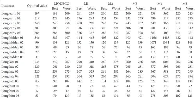
Table 7: Continued.

Instances Optimal value MODBCO M1 M2 M3 M4 M5

Best Worst Best Worst Best Worst Best Worst Best Worst Best Worst

Long early 01 197 194 209 241 259 200 222 200 221 339 362 220 243 Long early 02 219 228 245 276 293 232 254 232 253 399 419 253 275 Long early 03 240 240 258 268 291 243 257 243 262 349 366 251 273 Long early 04 303 303 321 336 356 306 324 306 320 411 430 319 342 Long early 05 284 284 300 326 347 287 310 287 308 383 403 301 321 Long hidden 01 346 389 407 444 463 403 422 403 421 4466 4488 422 442 Long hidden 02 90 108 126 132 150 120 139 120 139 1071 1094 128 148 Long hidden 03 38 48 63 61 78 54 72 54 75 163 181 54 79 Long hidden 04 22 27 45 49 71 32 54 32 51 113 132 36 58 Long hidden 05 41 55 71 78 99 59 81 59 70 139 157 60 83 Long late 01 235 249 267 290 310 260 278 260 276 588 606 262 286 Long late 02 229 261 280 295 318 265 278 265 281 577 595 263 281 Long late 03 220 259 275 307 325 264 285 264 285 567 588 272 295 Long late 04 221 257 292 304 323 263 284 263 281 604 627 276 294 Long late 05 83 92 107 142 161 104 122 104 125 329 349 118 138 Long hint 01 31 40 58 53 73 44 67 44 65 126 150 50 72 Long hint 02 17 29 47 40 62 32 55 32 51 122 145 36 61 Long hint 03 53 79 137 117 135 85 104 85 101 278 303 102 123

If the obtained significance value is less than the critical value (0.05), then the null hypothesis is rejected, and thus the alternate hypothesis is accepted. Otherwise, the null hypothesis is accepted by rejecting the alternate hypothesis.

6.3.2. Duncan’s Multiple Range Test. After the null hypothesis is rejected, to explore the group differences post hoc or multiple comparison test is performed. Duncan developed a procedure to test and compare all pairs in multiple ranges [42]. Duncan’s multiple range test (DMRT) classifies the significant and nonsignificant difference between any two methods. This method ranks in terms of mean values in increasing or decreasing order and group method which is not significant.

6.4. Experimental and Result Analysis. In this section, the effectiveness of the proposed algorithm MODBCO is com-pared with other optimization algorithms to solve the NRP using INRC2010 datasets under similar environmental setup, using performance metrics as discussed. To compare the results produced by MODBCO seems to be more competitive with previous methods. The performance of MODBCO is comparable with previous methods listed in Tables 7–18. The computational analysis on the performance metrics is as follows.

6.4.1. Best Value. The results obtained by MODBCO with competitive methods are shown in Table 7. The performance is compared with previous methods; the number in the table refers to the best solution obtained using the corresponding algorithm. The objective of NRP is the minimization of cost; the lowest values are the best solution attained. In the evaluation of the performance of the algorithm, the authors

Table 8: Statistical analysis with respect to best value.

(a) ANOVA test

Source factor: best value Sum of squares df Mean square 𝐹 Sig. Between groups 1061949 5 212389.8 3.620681 0.003 Within groups 23933354 408 58660.18 Total 24995303 413 (b) DMRT test

Duncan test: best value

Method 𝑁 Subset for alpha = 0.05

1 2 MODBCO 69 120.2319 M2 69 124.1304 M5 69 128.087 M3 69 129.3478 M1 69 143.1594 M4 69 263.5507 Sig. 0.629 1.000

have considered 69 datasets with diverse size. It is apparently shown that MODBCO accomplished 34 best results out of 69 instances.

The statistical analysis tests ANOVA and DMRT for best values are shown in Table 8. It is perceived that the significance values are less than 0.05, which shows the null hypothesis is rejected. The significant difference between

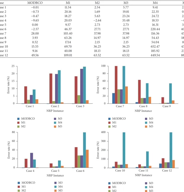
Table 9: Experimental result with respect to error rate. Case MODBCO M1 M2 M3 M4 M5 Case1 −0.01 11.54 2.54 5.77 9.41 2.88 Case2 −0.73 20.16 1.69 19.81 22.35 0.83 Case3 −0.47 18.27 5.63 23.24 24.72 2.26 Case4 −9.65 20.03 −2.64 33.48 18.53 −4.18 Case5 0.00 9.57 2.73 2.73 16.31 3.93 Case6 −2.57 46.37 27.71 27.71 220.44 40.62 Case7 28.00 105.40 37.98 37.98 116.36 45.82 Case8 3.93 63.26 14.97 14.97 54.43 18.00 Case9 0.52 17.14 2.15 2.15 54.04 8.61 Case10 15.55 69.70 36.25 36.25 652.47 43.25 Case11 9.16 40.08 18.13 18.13 185.92 23.41 Case12 49.56 109.01 63.52 63.52 449.54 88.50

Case 4 Case 5 Case 6

NRP Instance MODBCO M1 M2 M3 M4 M5 0 20 40 60 80 Er ro r ra te (%)

Case 10 Case 11 Case 12

NRP Instance MODBCO M1 M2 M3 M4 M5 0 100 200 300 400 Er ro r ra te (%)

Case 7 Case 8 Case 9

NRP Instance MODBCO M1 M2 M3 M4 M5 0 20 40 60 80 100 Er ro r ra te (%)

Case 1 Case 2 Case 3

NRP Instance MODBCO M1 M2 M3 M4 M5 0 5 10 15 20 25 Er ro r ra te (%)

Figure 7: Performance analysis with respect to error rate.

various optimization algorithms is observed. The DMRT test shows the homogenous group; two homogeneous groups for best values are formed among competitor algorithms.

6.4.2. Error Rate. The evaluation based on the error rate shows that our proposed MODBCO yield lesser error rate compared to other competitor techniques. The computa-tional analysis based on error rate (%) is shown in Table 9 and out of 33 instances in sprint type, 18 instances have achieved zero error rate. For sprint type dataset, 88% of instances have

attained a lesser error rate. For medium and larger sized datasets, the obtained error rate is 62% and 44%, respectively. A negative value in the column indicates corresponding instances have attained lesser optimum valve than specified in the INRC2010.

The Competitors M2 and M5 generated better solutions at the initial stage; as the size of the dataset increases they could not be able to find the optimal solution and get trapped in local optima. The error rate (%) obtained by using MODBCO with different algorithms is shown in Figure 7.