Abstract—The ability of load to respond to short-term varia-tions in electricity prices plays an increasingly important role in balancing short-term supply and demand, especially during peak periods and in dealing with fluctuations in renewable energy supplies. However, price responsive load has not been included in standard models for defining the optimal scheduling of genera-tion units in short-term. Here, elasticities are included to adjust the demand profile in response to price changes, including cross-price elasticities that account for load shifts among hours. The resulting peak reductions and valley fill alter the optimal unit commitment. Enhancing demand response also increases the amount of wind power that can be economically injected. Fur-ther, wind power uncertainty can be managed at a lower cost by adjusting electricity consumption in case of wind forecast errors, which is another way in which demand response facilitates the integration of intermittent renewables.
Index Terms—Wind power generation, demand response, real-time pricing, unit commitment
I. INTRODUCTION
omplex operational decisions have to be made in electric power markets. In time frames of one hour to one week ahead, mixed-integer and often nonlinear Unit Commitment (UC) models are applied to determine which units should be turned on and off [1]. Generation outputs are adjusted to load to maintain the system power balance. These optimization models are used to minimize generation costs or maximize profits, taking into account operational constraints.
Typically, fixed hourly electric load levels, based on short-term forecasts, are assumed in UC models. However, the on-going roll-out of smart meters, which allow communication of short-term electricity prices, creates opportunities for greater participation of demand in electricity markets. Therefore, UC models should be enhanced to account for adjustments of electricity consumption levels in response to frequently com-municated electricity prices. Demand-side participation can increase market efficiency (measured by net economic sur-plus) by reducing loads when marginal benefits of tion are less than marginal costs, and by increasing consump-tion when the reverse is the case. Net economic surplus (or social surplus) is widely used by economists in benefit-cost analyses, and is calculated here as the sum of consumer
sur-C. De Jonghe and R. Belmans are with the research group Electa (ESAT), Katholieke Universiteit Leuven, Belgium (e-mails: Cedric.DeJonghe @esat.kuleuven.be and [email protected]). B.F. Hobbs is with the Johns Hopkins University, Baltimore, MD 21218 USA (e-mail: [email protected]). Dr. Hobbs is supported by the US National Science Foun-dation under grants EFRI 0835879, OISE 1243482, ECCS 1230788 and by the USDOE Consortium for Electric Reliability Technology Solutions.
Manuscript received February XY, 2012
plus (net benefits to consumers) and producer surplus (profit). Additionally, the impact of wind power variability and limited predictability may be reduced by demand response, which must be accounted for in assessments of the value of smart meters and real-time prices.
UC models generally simplify or neglect the demand-side. However, some models include demand-side bidding, a mech-anism that enables consumers to actively participate in elec-tricity trading, typically on power exchanges. This is facilitat-ed by consumers allowing their loads to be reschfacilitat-edulfacilitat-ed in order to balance supply and demand or to maintain security requirements [2]. A day-ahead market-clearing tool offering consumers the opportunity to reduce their energy costs by submitting a shifting bid has been presented in [3].
Some UC models incorporate non price-based demand re-sponse such as Direct Load Control (DLC). The impact of DLC on UC decisions and the potential saving of using DLC as system spinning reserve are illustrated in [4]. DLC is in-cluded in a UC model in [5] with a focus on air conditioning loads. In [6], deferrable loads are coupled with the supply of renewable energy generation, using dynamic programming; however, that paper disregards the elasticity of the demand-side and the corresponding consumer surplus. An alternative approach to represent responsive load is to explicitly model consumers’ optimal decision making, explicitly considering timing and amount of use, e.g., about storage or deferring loads. However, this would result in a bilevel modeling struc-ture for a UC model, in which generator schedules are opti-mized subject to the optimal solutions of consumer problems; such MPECs (mathematical programs with equilibrium con-straints) are difficult to calibrate and solve. However, some energy market equilibrium models, such as the USDOE Na-tional Energy Modeling System, do explicitly account for the effect of price changes on consumer energy equipment in-vestment and operations [7].
In this paper, demand elasticity is used as an approximation to a often complex consumer decision making process, involv-ing reschedulinvolv-ing of energy usinvolv-ing activities. The complexity of consumer decision making process results from the both social and technical aspects. Social aspects refer to the fact that price changes might have a different effect during different mo-ments (hour of the day, weekday versus weekend, season, ...), depending on exact energy uses and varying flexibility over time in adjusting those uses. Technical aspects refer to the fact that some demand adjustments can only be made during a limited period of time, that only a limited amount of consump-tion (and related appliances) can be shifted. Both effects com-bined might yield non-linear and time-varying response, re-stricted by saturation effects and having minimum and maxi-mum response levels. Models that represent demand response
Value of Price Responsive Load
for Wind Integration in Unit Commitment
Cedric De Jonghe, Benjamin F. Hobbs, Fellow, IEEE, and Ronnie Belmans, Fellow, IEEE
with own- and cross-price elasticities can be viewed as first-order approximations to such more complex representations.
Some approaches that can be taken to parameterizing these models include the following. First, empirical estimates of elasticities and cross-elasticities from pilot studies of demand response programs can be extrapolated from pilot studies [8]. An example is the Baltimore Gas & Electric peak-time rebate and critical peak pricing pilot, which found a 20-30% load decrease in five afternoon hours from a ten-fold effective increase in price (an own price-elasticity of about -0.025), but at the same time ~3-8% increases in load in the hours immedi-ately preceding and following those hours (which is a cross-price elasticity with respect to each other hour’s cross-price of less than +0.01, but which in aggregate is significant) [9]. If this is the only source of demand response, such results could be extrapolated; for example, if 50% of residential consumers are assumed to participate, and consumer load is 40% of demand in those hours, then those elasticities could be multiplied by 0.5*0.4 = 0.2 to obtain the equivalent elasticity for aggregate load. Second, the impacts of new demand response technolo-gies, such as plug-in hybrids or electric vehicles, could be approximated based on metamodeling analyses of the results of engineering studies. As an example, sensitivity analysis of detailed optimization or simulation models of vehicle charging behavior could be used to assess how charging would change with changes in relative prices [10], [11]. Again, the implica-tions for aggregate load elasticity could be assessed by extrap-olating, based on assumptions about the market penetration of the new technologies and the individual load shapes and re-sponsiveness. Third, judgment could be used to limit the amounts of change in loads that are allowed. For instance, if a large part load response is from altering use of air condition-ing or other HVAC systems, the changes in loads that might be expected from demand response could be bounded by hy-pothesizing based on reasonable assumptions about tolerable temperature changes, informed by experience from load con-trol and pilot demand response studies.
Own-price elasticity (εt), also referred to as self-elasticity
[12], indicates the relative change in the demand for electricity in response to a change in its price, where p0,t and q0,t are
re-spectively the initial price and loads in hour t: 0, 0, t t t t t p q p q (1)
The own-price elasticity represents the willingness of con-sumers to adjust their electricity demand and is typically nega-tive. Meanwhile, the cross-price elasticity (εt,t’) indicates the
change in demand for electricity in hour t in response to a change in the price for electricity in hour t’≠t:
0, ' , ' ' 0, t t t t t t p q p q (2)
Own-price elasticities are used in an electricity market sim-ulator to study consumer response in [13]. Cross-price elasticities are used in dynamic electricity pricing models in [14]. The impact of real-time pricing with own-price elasticities on the use of wind power generation and the fre-quency of generation units being ramp-up or down-constrained in a UC model is studied in [15]. However, the impact on operations costs, such as energy, start-up, emission, and wind power curtailment costs, is not reported. Unlike our
study, cross-price elasticities and forecast uncertainty are also not considered. The effect of forecast errors is included in [16], without considering demand response to changes in electricity prices. The impact of demand response on wind integration is analyzed using stochastic programming in [17]. This paper does not include cross-price elasticities, and does not examine the impact on different cost components such as fuel and start-up costs.
In this paper, we first present a fixed demand UC model in which consumers face a uniform price over the entire time horizon. This solution is obtained from a standard cost-minimizing UC model; we then calibrate hourly demand curves based on the original loads, assumed elasticities, and a price based on the hourly (load weighted) marginal costs from the cost-based model. These demand functions with own- and cross-price elasticities are then used in a modified UC model to represent demand response in section II, describing the impact on wind curtailment, carbon emissions and market efficiency (gauged by net economic surplus). In section III, the assumption of perfectly predictable wind power injections is relaxed in the model by including wind power stochasticity, followed by conclusions in section IV.
II. UNIT COMMITMENT WITH PRICE RESPONSIVE LOAD
Assuming a single market clearing price in each time inter-val (perhaps differentiated over space, as in nodal pricing models), UC models can be modified to find the equilibrium supply-demand balance and price for each interval. Under some conditions, described below, maximization of the market surplus (producer, consumer, and, in the case of transmission constraints, transmission operator surplus), [18] simulates the outcome of a competitive market, consistent with Samuelson's principle [19], assuming that submitted bids represent supplier costs and consumer benefits. If there are no cross-price elasticities, surplus is defined as the integral of the demand function minus the generation cost of meeting the load, taking operational constraints into account. According to microeco-nomic theory, price-taking end-users who are maximizing their net benefits of consumption (i.e., consumer surplus) increase their load up the point where the cost of consumption is equal to the marginal benefit of that consumption [20]. A. Model description
A general UC model with fixed loads is described in detail in [21]. The specific formulation of the UC model applied in this paper can be found in [22] and is summarized in the Ap-pendix. This model optimizes the commitment and dispatch of power generating units in the electricity system by minimizing operating costs. The operating costs include variable genera-tion, start-up and wind power curtailment costs. Both fuel and emission costs are included in the variable generation costs. Generation technology-specific carbon emissions are included and multiplied by an emission price. Commitment of genera-tion units also involves a technology specific start-up cost whenever a unit is turned on. Excessive wind power injections in the system could result in overgeneration situations. Clear-ly, those situations with excess wind power occur when the amount of wind power injected (plus output from thermal generators running at their minimum allowable outputs) ex-ceeds the load. Reducing hourly wind power injections in order to prevent such situations is referred to as wind power
curtailment. For each MWh of wind power curtailment, a cost is incurred. Although it can be argued that the true market cost of wind curtailment is zero, private costs to wind providers can be significant (in terms of lost production tax credits or renewable energy credits). Finally, a real-time system power balance requirement is enforced.
This reference model is extended to model price-responsive load. The model results define the optimal (primal) variables. The marginal price of electricity is found based on the shadow price of the system power balance requirement. This is defined as the dual variable that results if the 0/1 commitment status of the generators is fixed, and the resulting linear program is solved for the optimal dispatch. This marginal price is then used to calculate an average energy price weighted by hourly energy demands for the entire time horizon. This is the flat tariff that we assume consumers face in the base case (no real-time pricing structure).1 The single tariff combined with the base case hourly loads defines a price-quantity pair for each hour through which each hour’s linear elastic demand function is drawn. Own- and cross-price elasticities are included, defin-ing decision variables (demt) equal to the load in each hour
(rather than being a fixed coefficient): ,
t i t t t
i
g WIND curt dem
t (3)The equilibrium solution considering short-term demand re-sponse represented by the linear elastic demand function can be found by reformulating the Mixed Integer Linear Program (MILP) model as a Mixed Integer Non-Linear Program (MINLP) [18]. The objective function would be the maximiza-tion of consumer and producer surplus. The objective funcmaximiza-tion terms represent the integral of the demand functions (in the case of demand functions with only own-elasticities or sym-metric cross-price coefficients) minus generation cost:
, ' ' ' 1 2 t t t t t t t t
Max dem E dem F dem
, , , ( ) t i i i t i t t i tg MC EP EMIS s_costs CC curt
(4)The first summation is the integral of the inverse demand function (price at hour t = Et + tFt,tdemt), which represents
the value of consumption. To obtain net social surplus, genera-tion costs (including marginal fuel costs, emissions penalties, start up costs, and wind curtailment costs) are then subtracted. (A full list of notation is provided in the Appendix.)
This model can be viewed as simulating a market equilibri-um in which the generation firm solves for its production schedule and calculates prices to which consumers react ac-cording to demand functions, known by the firm. This is a type of Stackelberg equilibrium in which the firm is the leader and the consumers are followers. In general, such a model is a mathematical program with equilibrium constraints (MPEC) [23]. However, because consumers react according to demand functions that are the basis of the benefits in the firm's objec-tive (4), the MPEC reduces to the above-described MINLP. Under the unrestrictive assumptions of (a) the existence of a
1 A similar methodology could be applied to calculate weighted average prices for a double tariff structure, with peak and off-peak periods [31].
feasible solution and (b) nonnegative generation costs and bounded quantities demanded, a finite optimal solution will exist to the MINLP, and therefore an equilibrium will exist.
According to the integrability condition, the coefficient ma-trix Ft,t’, must be symmetric to use the QP approach.
Addition-ally, MINLPs can be hard to solve. For these reasons, an alter-native computational procedure based on the PIES algorithm is attractive and used here. The PIES algorithm is compared with other methods in [24], which focuses on a long-term investment planning optimization, as opposed to the short-term operational impacts that are the focus of this paper.
This algorithm can approximate a non-integrable problem by a sequence of MILPs that account for both own- and cross-price elasticities.2 This approach uses a piecewise linearization of the price elastic demand function. The MILPs can be solved by efficient optimization software [25] and do not require a coefficient matrix Ft,t’ with symmetric cross-price terms.
Elsewhere, the PIES algorithm is shown to converge for en-ergy supply models that are pure LPs [26], however, there is no such proof available for MINLPs such as ours. In the ab-sence of such a proof, our use of the PIES algorithm should be viewed as a heuristic approach to modeling the response of demand with cross-price elasticities within a market with integer constraints. The mechanics of the PIES algorithm as applied here are described in section V. Appendix.
B. Data and assumptions
Here, we use the basic model to calculate the cost-minimizing commitment of generation units in a system with high wind penetration for an illustrative 48-hour period. Ener-gy demand data is based on an hourly load profile given in the “6 bus hourly data” file, available at http://motor.ece.iit.edu/ Data/. This website gathers multiple datasets used in several papers, e.g., [27] and [28]. The wind power profile captures its variability in a realistic manner as it is based on historical data (http://www.energinet.dk/). In the first six hours, available wind power exceeds electricity demand. Demand and power generation is assumed to be located in a single node; else-where, we present results for a transmission-constrained UC problem [22]. In this section, perfect foresight is assumed with respect to real-time wind power injections as well as consum-ers’ demand and their responsiveness to electricity prices.
In reality the generation firm, required to balance injections and offtakes, might face significant uncertainty regarding the response of consumers to price changes. Errors in estimating demand elasticities would be on top of the 2-5% errors com-mon in day-ahead load forecasting, and the even larger errors in wind forecasting. As is well known, such forecast errors increase the cost of system operations [29]. Thus, our model may overstate the ability of utilities to take optimal advantage of demand response.3 In section III, we consider the stochastic case on wind injections. Five technologies are represented, inspired by the 24-bus IEEE Reliability Test System [30] and
2 This linear approximation method has good convergence characteristics. In the UC model, 20 piecewise steps have been created at each side of the initial demand level to represent the demand curve. The step size of the piecewise integration is reduced by a factor of 1.5 in each iteration. After 15 iterations, the objective value changes by less than 0.01% in consecutive iterations.
3
The inclusion of different uncertainty in demand elasticity will be modeled as multiple scenarios in stochastic unit commitment in further research.
a modified IEEE 118-bus Test System [27]. The power system portfolio is composed of 19 generation units (Table I). Two nuclear and two coal-fired power units are assumed, as well as three CCGT units. Nuclear power units have the lowest mar-ginal operating cost, but are less flexible, having a slow ramp-ing rate and a minimum run requirement statramp-ing that their output is always at or above their PMIN. Coal-fired and closed-cycle gas turbine (CCGT) units typically face shorter minimum on- and down-times. Finally, six Oil-fired Combus-tion Turbines (OCT) and six Gas-fired CombusCombus-tion Turbines (GCT) are the peaking units, being the most flexible units in the system. Carbon emissions are taken into account, given the carbon content of the fuel and an average technology efficien-cy. The price of carbon emissions is considered to be 10 €/tonne CO2. Finally, the option of spilling wind power is allowed at a penalty of 30 €/MWh. (This penalty represents the subsidy that the wind producer foregoes, and lies between the German feed-in tariff (in the neighborhood of 70 €/MWh) and the US federal production tax credit which was recently renewed (less than 20 €/MWh).) The basic model is then ex-tended using own-price elasticities between 0 and -0.30. An overview of short-term price elasticity levels is given in [31] ranging between -0.002 to -0.158. Short-term elasticity levels in the same order of magnitude are suggested in [8].
TABLE I
UNIT SPECIFIC OPERATIONAL PARAMETERS
Nuclear Coal CCGT GCT OCT
PMAX [MW] 400 300 250 30 30 PMIN [MW] 100 100 75 5 10 EMIS [tonne/MW] 0 0.9 0.41 0.59 0.78 MC [€/MWh] 10 35 50 72 (150)4 110 SC [€/start] 1000 800 500 80 75 RAMP [MW/hr] 33 40 50 100 100 MO [hr] 8 5 2 1 1 MD [hr] 8 5 2 1 1 Number of units 2 2 3 6 6
Other publications indicate that residential consumers are even more responsive, such as listed in [32], [33] and [34], between -0.18 and -0.79. The comparison of model results for alternative elasticity levels shows the sensitivity of the results with respect to the price elasticity. Positive cross-price elasticities are included, so that a price increase in one hour (which would decrease load in that hour due to the negative own-price elasticity) would result in load increases in other hours, as consumers respond to a higher price in one hour by shifting part of their load to adjacent hours. Sensitivity anal-yses are undertaken assuming symmetric cross-price elasticities of 0.02, in which a price change in a given hour can equally affect loads in 1 up to 3 hours before and after the hour [35].
C. Model results
Here we compare optimal generation, power prices, opera-tions costs, environmental benefits and wind curtailment for alternative price elasticities, including zero (the base model).
4 An additional Gas-fired Combustion Turbine (GCT) with a marginal operat-ing cost of 150 €/MWh is included as a back-up option in case of restricted available power generation capacity.
1) Generation outputs
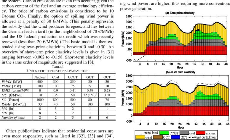
In the UC model without demand-side flexibility, Fig. 1a shows that wind is curtailed by more than 500 MW in hours 1-7, resulting in prices of -30 €/MWh. It takes at least three hours before the nuclear power units reach rated capacity as enforced by the 33%/hr ramping limit. Two coal-fired power units are turned on in hour 8 and are restricted by their 40%/hr ramping limit. A first and second CCGT unit are turned on in hour 14 and 18 respectively, in response to peaking loads. Even though the demand peak is less pronounced between hours 32 and 36 compared to hour 20, net loads, after subtract-ing wind power, are higher, thus requirsubtract-ing more conventional power generation.
Fig. 1: Generation outputs and loads: (a) Zero price elasticity (base); (b) -0.20 own price elasticity
Finally, generation in hours 27 and 28 also require special attention. Reduced conventional energy loads during the night cause one coal-fired unit to be turned off. It takes five hours before this unit can be turned on again, due to its minimum down-time. At the same time, the output of the other coal-fired power unit is reduced to the minimum level of 100 MW. Also the output of the nuclear power unit is slightly reduced.
In contrast, Fig. 1b shows the generation outputs given a
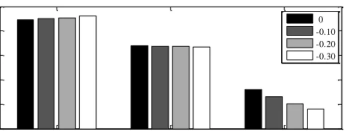
0.20 own-price elasticity. Looking at the first 8-hour period, loads are increased by about 500 MW. Simultaneously, initial peak load levels are reduced by almost 300 MW or 10% be-tween hours 18 and 22. Valley fill effects during the first hours of this period allow an earlier start-up of the nuclear power units. Valley filling also occurs during the off-peak period between the first and the second 24-hour period, espe-cially around hours 27-28. The increased generation from the nuclear unit also significantly increases its capacity factor (the ratio of actual energy generated by a unit to the maximum possible energy) (Fig. 2).
CCGT units are typically used to satisfy demand for elec-tricity during higher load periods. CCGT generation is reduced when increasing demand-side flexibility. Furthermore, it is no longer necessary to turn on a second CCGT unit in the first 24-hour period. Loads are also reduced at the peak load period during hours 32-44 by about 150 MW. As a result, not only the CCGT output is reduced, but also the third CCGT unit is switched off after hour 35, reducing its capacity factor.
Fig. 2: Capacity factors for nuclear, coal-fired and CCGT power units under alternative demand elasticities (0=base case)
2) Electricity prices
First we discuss marginal costs from the base solution, which are also the prices in the zero elasticity, real-time pric-ing case. Afterwards, those are compared with the marginal cost (price) in the -0.20 own-price elasticity case.
The real-time marginal price for the UC model without re-sponse is shown by the solid line in Fig. 3. The coal-fired unit is the marginal unit in hours 9-14 and 29-31, yielding a price equal to its marginal cost of 44 €/MWh. This cost equals the coal fuel cost of 35 €/MWh plus an emissions cost of 9 €/MWh (0.9 tonne CO2/MWh times the CO2 emission price of 10 €/tonne). A CCGT is the marginal power source in hours 15-24 and 36- 46. Its marginal cost, including fuel and emis-sions, yields an electricity price of 54.1 €/MWh. Similarly, the electricity price when the GCT or OCT are marginal results in electricity prices of 77.9 €/MWh (hour 33 and 35) and 117.8 €/MWh (hour 34), respectively. During hours of wind power curtailment, the price of electricity becomes negative in the base solution, because increasing electricity demand by one MWh reduces curtailment costs by 30 €/MWh. For some other hours, prices spike up or down because of the interaction of ramp constraints with dispatch (e.g., hours 8 and 28). A spike up can occur when a load increase in a given period not only increases generation in that period but also forces substitution of costly generation for cheaper in an earlier period. This hap-pens because a binding ramp constraint is forcing the cheaper generator downward in order to make it possible for the sys-tem to attain the required ramp level [36].
Fig. 3: Comparison of real-time price of electricity to flat tariff
In the extended model, we assume that consumers react when prices deviate from the base (flat) tariff. This flat tariff of 42.7 €/MWh is calculated as the quantity-weighted average electricity price for the UC model without demand response. Market-clearing hourly electricity prices with -0.20 own-price elasticity are compared to the flat tariff in Fig. 3. The latter prices are not the same as the marginal costs under zero price elasticity because of shifts in demand (valley-fill and peak-reduction) result in different generation units being on the margin. This generally makes prices less extreme, and erases the price spikes associated with high ramps.
3) Operations costs
Price-based demand response also impacts operations costs (Table II). Increasing the assumed level of own-price elasticity from -0.10 to -0.30 reduces total operations costs by approxi-mately 10% to 20% in this 48-hour period. The inclusion of cross-price elasticities, representing shifting of electricity consumption, decreases the operations cost reductions, be-cause negative own-price elasticities are counteracted by posi-tive cross-price elasticities. For instance, if price increases in one hour, demand is dampened in that hour, but there is offset-ting increases in loads in other hours. These cross-price effects mean that the cost savings are appreciably less than if only own-effects are assumed. Table II shows that when the great-est amount of cross-price effect is assumed, the cost savings relative to the zero elasticity case is roughly 60% compared to the own-price elasticity only case.
4) Carbon emissions and wind curtailment
Price-based demand response can have environmental bene-fits. Demand response reduces net load variance, causing the more efficient units to generate more, although that does not always mean the cleanest units [37]. In this example, however, nuclear power units increase their output, while the power output of the polluting CCGT unit is reduced. Price response yields CO2 emission reductions of 5 to 10% relative to initial emissions. Price responsive consumers also facilitates wind integration. Hourly wind power spillage of 21% in the refer-ence scenario is reduced to about 7% in hour 2 and 3, assum-ing only a -0.10 own-price elasticity. With a -0.20 own-price elasticity or greater, wind is no longer curtailed.
TABLE II
OPERATIONS COSTS AND ENVIRONMENTAL BENEFITS UNDER ALTERNATIVE PRICE ELASTICITIES
Own elast. Total costs [€] Fuel costs [€] Start-up costs [€] Emissions [tonne] Curtailment [MWh] -0.00 1,930,439 1,631,733 7,370 22,489 2,215 -0.10 1,740,739 1,509,056 6,900 21,384 365 -0.20 1,618,328 1,407,201 6,400 20,474 0 -0.30 1,536,919 1,332,857 6,400 19,767 0
-0.20 own- with ± 1, 2, 3 hours of +0.02 cross-price elasticity
1 h 1,657,253 1,442,324 6,900 20,803 0
2 h 1,692,533 1,473,885 6,900 21,097 26
3 h 1,731,282 1,506,795 6,900 21,308 150
5) Impact on market efficiency
The general impact of consumers adjusting electricity con-sumption in response to short-term dynamic pricing on eco-nomic surplus (consumer plus producer surplus) is described in [38]. Model results in Table III show the welfare impacts of increasing the own-price elasticity of electricity demand for
Nuclear Coal CCGT 0 20 40 60 80 100 C apa ci ty fa ct or [ % ] 0 -0.10 -0.20 -0.30 5 10 15 20 25 30 35 40 45 -20 0 20 40 60 80 100 120 Hour [€/ M W h] No demand response Flat tariff -0.20 own elasticity
the 48 hour period. On average, consumption benefits (integral of the demand curve) are reduced as load shrinks, but total cost is reduced even more. Consequently, total surplus (and thus market efficiency) grows as the own-price elasticity is increased. We also express these changes in generation costs and surplus as a proportion of the generation costs in the ‘no response’ case. Table III suggests that generation costs can be reduced by as much as 20%, assuming a -0.30 own-price elas-ticity. But total surplus improves less (just 10.14%), because consumption benefits also decrease.
TABLE III
IMPACT OF OWN-PRICE ELASTICITIES ON WELFARE
Own-price elasticity -0.10 -0.20 -0.30
Consumption benefit change [€] -87,071 -149,651 -197817
Generation cost change [€] -189,700 -312,111 -393,520
Total surplus change [€] 102,628 162,460 195,703
Generation cost change [%] -9.83% -16.17% -20.38%
Total surplus change [%] 5.32% 8.42% 10.14%
III. DEMAND RESPONSE WITH WIND POWER STOCHASTICITY
This section departs from the assumption of perfectly pre-dictable wind power injections. The UC model is extended so that commitment decisions account for possible wind forecast errors in later periods. As a result, the model automatically commits additional reserve capacity to maintain reliable sys-tem operation in case forecasts are wrong. Also, in case wind power injections are underestimated, the UC solution main-tains downward ramp capability. But flexible generation may be more costly than other types of thermal generation; as a result, commitment of too much flexible capacity may in-crease system costs more than necessary [39]. Actual dispatch and demand response is then determined in real-time, when the wind output is known. Depending on the real-time wind power injection, a different price is sent to the consumers, resulting in scenario-specific levels of electricity demand, under the assumption that consumers can react to real-time prices.5
A. Model extension
The first step in including uncertainty about the real-time wind power injection in the system involves formulating a stochastic mixed-integer linear programming (MILP) model. Stochasticity is represented by a scenario tree for possible wind power generation forecasts for each individual hour as in [40], which like [31] does not consider the effect of price-responsive consumers. The inclusion of stochasticity means that scenario-specific parameters as well as scenario-specific decision variables must be defined, indicated by index j [41]. Hourly wind power injections become scenario-specific (windt,j). An equal probability is assigned to each of the three
scenarios (PRj = 1/3), as in [42]:
Scenario 1: Overestimate: less wind injected in real-time
Scenario 2: Wind power correctly forecasted
Scenario 3: Underestimate: more wind injected in real-time However, because of the size of a model with a full scenario tree with all combinations of all scenarios would be very large
5 Actual dynamic pricing mechanisms usually involve communication of day-ahead prices rather than real-time prices to consumers. The assumption here is that real-time prices are communicated, reflecting actual wind conditions, and then reacted to by consumers. Including a lag between forecast and actual prices in the UC is possible, e.g., by making decision about load levels at the same time as UC decisions rather than when dispatch decisions are made.
[32], we simplify the stochastic structure by assuming that each of the three scenarios in a given hour could occur, so that the unit commitment is optimized day-ahead recognizing that all three possibilities could occur. Ramp requirements or commitments of short-start units for each scenario are satis-fied, assuming that Scenario 2 occurs in the previous hour. This could be viewed as a simplification of a more extensive stochastic unit commitment that considers changes in load from all possible scenarios in a previous hour, but such a Mar-kov representation greatly increases the size of the problem. Our representation is a compromise between the need for computational efficiency and the desire to capture uncertainty across a range of possible ramps and load changes from hour to hour. This allows modeling of the effects of uncertainty without resulting in an explosive number of wind scenarios.
A sensitivity analysis calculates the impact of forecast er-rors for 4 alternative cases, respectively with the three scenar-ios of a correct forecast, an over- and underestimate of 10%, 15%, 20% and 25% in each hour of the projected wind power injections, corresponding to experience in Western Denmark for day-ahead forecasts, meaning 13 up to 37 hours ahead [43]. In a stochastic program, decision variables are divided into first-stage (‘here-and-now’) and later stage (‘wait-and-see’) variables as illustrated by Fig. 4. The here-and-now variables represent commitments made before it is known which scenario will occur, while the ‘wait-and-see’ variables are scenario-specific, chosen once the scenario is known in hour t. So-called ‘non-anticipativity’ constraints ensure that the here-and-now variables are the same for all scenarios.
Fig. 4: Decision tree for stochastic two stage problem
Here-and-now variables include the 0-1 binary variables that represent nuclear, coal-fired and CCGT commitments (zt,i). These commitments are assumed to be made day-ahead.
Thus, the on or off status of these units is assumed to be fixed for all scenarios for a given hour (non-anticipativity).
Wait-and-see variables are the four scenario-specific sets of primal variables defined for decisions that are deferred until the wind scenario is known. These include the amount of wind power curtailment (curtt,j); the thermal unit dispatch variables
(gt,i,j); OCT and GCT commitments; and responsive load
lev-els. The net load that must be met is scenario-specific, so each scenario j in each hour t has a separate set of recourse varia-bles. Generation for each unit in each of the scenarios in a given hour must satisfy ramp limits (RAMPi), assuming that
the scenario 2 solution has occurred in the previous hour (t-1): , , 1, ,2 t i j t i i i g g RAMP PMAX t i j, , (5) , , 1, ,2 t i j t i i i g g RAMP PMAX t i j, , (6) The scenario-specific GCT and OCT unit status variables also require a scenario-specific start-up cost (SCt,i,j). The resulting
scenario-specific costs are included in the objective function, which weights costs by the assumed probability PRj:
, , , , , ( ) j t i j i i t i j t i t i Min PR g MC EC EMIS SC
, , , j t j j t,i,j t j t j PR CC curt PR SC
(7)There are also scenario-specific constraints; in particular, power balances in each j guarantee that power injected and consumed is equal in every hour for every scenario:
, , , , ,
t i j t j t j t j
i
g WIND curt dem
t j, (8)Its dual variable is the scenario-specific electricity price. Then, assuming price-based demand response, scenario-specific prices finally yield scenario-specific hourly electricity loads, which are the fourth set of scenario-specific primal variables. B. Stochastic model results
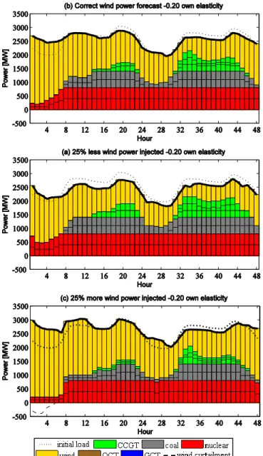
The introduction of price-based demand response in the model with wind power uncertainty impacts optimal genera-tion and the corresponding market-clearing equilibrium prices. We also compare costs, emissions and wind curtailment for the cases with and without price-based demand response. 1) Generation outputs
Generation outputs in Fig. 5 illustrate the impact of de-mand-side flexibility, assuming a -0.20 own price elasticity. Each of the scenarios has a probability of occurrence of 1/3, satisfying operational constraints assuming Scenario 2 in the previous hour. In the correct forecast case, loads are increased by up to 500 MW in the first hours because of negative prices, relative to the initial load level. During the other hours, load is less significantly impacted because prices are closer to the flat tariff. The price responsive load profile rarely deviates in later hours more than 100 MW from the base levels. In this case, several generation units are committed, providing reserve capacity to deal with the wind power overestimation case.
The wind power overestimation case (scenario 1) is where the amount of realized wind power is 25% less than forecast-ed. With consumers responding to real-time price signals, this deficit can be offset by increasing conventional power genera-tion outputs or by lowering real-time electricity loads. Fig. 5a suggests that demand is reduced compared to the initial load (dashed line) when less wind power is realized in real-time. For instance, demand drops by 340 MW and 400 MW, absorb-ing 85% and 100% of the forecast error in hours 9 and 8, re-spectively. This means that in some hours, the entire amount of required flexibility in the system is provided by the de-mand-side. On average, more than 45% of the forecast errors in scenario 1 are resolved by the demand-side. By reducing loads, GCT and OCT power generation is avoided, which also saves significant amounts of fuel expenses and lowers prices.
Fig. 5: Generation outputs with wind uncertainty
The wind underestimation case (scenario 3) is where 25% more wind power arrives in real-time than is forecasted. When consumers are able to respond to real-time price signals, this surplus can be offset by lowering conventional power genera-tion outputs or by increasing real-time electricity loads. Lower prices motivate consumers to use more power compared to the initial load (dashed line in lower graph). Between hours 9-13, real-time hourly electricity loads are increased by about 200 MW, absorbing more than 50% of the wind power injection surplus. Demand response also allows the nuclear power unit to operate at capacity. On average, more than 25% of the fore-cast errors in scenario 3 are absorbed at the demand-side. 2) Electricity prices
Electricity prices are shown in Fig. 6 for the three wind forecasting scenarios. Electricity prices in the upper graph (a) (without demand response) can be explained by the marginal generator in each hour. Prices are commonly higher when less wind power is injected. For instance, in hour 34 with scenario 1, the back-up GCT unit must be started-up with marginal costs of 155.9 €/MWh, including emission costs.
Fig. 6: Electricity prices with wind power uncertainty: with and without price elastic demand
With price responsive load (Fig. 6b), higher prices still oc-cur when less wind power is injected. However, the differ-ences in prices between the correct forecast scenario and the other two cases are reduced. This directly relates to ability of demand response to eliminate the need to dispatch peaking units, reducing upward price spikes. Also, the amount of wind power curtailment is reduced.
3) Operations costs
Operations costs, carbon emissions and wind power cur-tailment levels are summarized in Table IV with and without price elastic demand, not only for the 25% forecast errors as in Figs. 5 and 6, but also for lesser amounts of forecast error. The results are expected values over the three scenarios (i.e., each weighted by 1/3, the assumed probability for each scenario). Without price-based demand response, expected operations costs are 2.7% to 5% higher relative to the analysis without forecast errors (Table II), assuming forecast errors ranging from 10% to 25%. This difference in total costs indicates the extent to which deterministic models underestimate the cost of wind power integration [44]. Larger forecast errors give higher fuel as well as start-up costs. This higher cost occurs for two reasons. One is that higher commitment costs are incurred for the nuclear/coal/CCGT units because more are committed than in the deterministic solution in order to accommodate the possibility of significantly higher net load. The second is that thermal generation costs are generally a convex function of net load, with the cost increase resulting from an increase in load being greater in magnitude than the cost decrease resulting from a similar decrease in load.
When consumers are able to adjust their loads, the system has more flexibility to deal with wind forecast errors. The demand flexibility means that the system can avoid dispatch-ing expensive generators and reduces partial loaddispatch-ing of power units. Consequently, expected costs are reduced by 10%, given
a 10% forecast error, and up to 15% for a 25% forecast error, assuming a -0.20 own-price elasticity. Consequently, demand-side participation is a way to reduce the cost of poor forecasts.
TABLE IV
EXPECTED OPERATIONS COSTS, EMISSIONS, AND WIND CURTAILMENT WITH WIND POWER UNCERTAINTY: WITHOUT PRICE-BASED DEMAND RESPONSE
Forecast error
Total costs
[€] Fuel costs [€] costs [€] Start-up Emissions [tonne]
Curtailment [MWh] Inelastic electricity demand
10% 1,945,090 1,643,486 8,123 22,520 2,276 15% 1,965,769 1,661,006 8,244 22,490 2,387 20% 1,999,534 1,687,788 8,803 22,560 2,578 25% 2,043,417 1,722,863 8,559 22,635 2,855 -0.20 own-price elasticity 10% 1,663,473 1,445,806 6,900 21,002 29 15% 1,652,165 1,433,896 6,900 20,796 120 20% 1,690,477 1,466,710 6,900 20,904 270 25% 1,700,182 1,471,263 6,900 20,843 460
4) Emissions and Wind Curtailment
When loads adjust in response to electricity prices, carbon emissions can be reduced by 6.5% to 8% assuming a 10% to 25% forecast error, respectively. Short-term price-based de-mand response reduces the amount of wind curtailment dra-matically. When loads cannot adjust in response to prices, an oversupply of wind must be increasingly curtailed with in-creasing forecast error. As suggested by the results in Table IV, wind variations can easily be absorbed by demand re-sponse. With zero elasticity, the total level of curtailment is 2,855 MWh under a 25% forecast error; in that case, a flexible demand-side can reduce curtailment by almost 85% to 460 MWh.
IV. CONCLUSIONS
UC models optimize short-term operation of available gen-eration units, accounting for technical constraints. In typical applications, loads are assumed to be fixed, so flexibility to adapt to demand or wind forecast errors must be provided by thermal generation. However, a smart meter roll-out plus real-time pricing facilitates demand-side flexibility. This provides economic value in the form of generation cost reductions and avoided wind power spillage, which we quantify in this paper.
We include price responsive load in a UC model. Consum-er’s ability to adjust load in response to price is modeled using hourly elastic demand functions. We represent their flexibility by own- and cross-price elasticities.
Increasing consumer responsiveness to price deviations on the one hand reduces peak loads, avoiding expensive peak load power generation. On the other hand, demand valleys with low electricity demand or excess wind power generation can be filled, increasing the output of less expensive power generation and providing additional benefits of consumption. Consequently, the capacity factor of base load generation increases, whereas peakers see reduced capacity factors. In addition to those cost reductions, the integration of non-dispatchable wind power generation is improved, measured by the amount of wind spillage avoided.
Positive cross-price elasticities, representing the shift of loads from high price to low price periods, are modeled using an iterative linearization technique based on the PIES algo-rithm. If there are such cross-price effects, disregarding them
4 8 12 16 20 24 28 32 36 40 44 48 -30 0 30 60 90 120 150 Hour P ri ce [ €/ M W h]
Electricity price: wind forecast scenarios without response 25% less injected correct forecast 25% extra injected 4 8 12 16 20 24 28 32 36 40 44 48 -30 0 30 60 90 120 150 Hour P ri ce [ €/ M W h]
Electricity price: wind forecast scenarios -0.20 own elasticity 25% less injected
correct forecast 25% extra injected (b)
in unit commitment modeling results in an exaggeration of cost savings from responsive demand.
Finally, a flexible demand-side proves to be effective in dealing with the unpredictability of real-time wind power injections. A stochastic UC model indicates that the costs of wind power forecast errors can be significantly reduced by demand-side flexibility. As the instantaneous system power balance no longer needs to be maintained by supply-side flex-ibility alone, greater amounts of wind power can be integrated into the system with fewer problems from forecast errors.
V. APPENDIX A. Nomenclature Sets Indices T Index of hours t T’ Index of cross-hours t’ I Generation technologies i J Index of scenarios j Parameters
E, F Parameters of the linear inverse demand func-tion P (as a funcfunc-tion of quantities demanded) with F symmetric elasticity matrix for own- and cross-price elasticity
CC Cost of wind power curtailment [€/MWh]
D Demand function
dem0 Initial demand level [MWh]
ε Price elasticity
EMIS Marginal emission [tonne CO2/MWh] EP Emission price [€/tonne CO2] MC Marginal generation costs [€/MWh]
MD Minimum down-times [h]
MO Minimum on-times [h]
P Inverse demand function p0 Reference price level [€/MWh]
PMAX Maximum output level [MW]
PMIN Minimum run level [MW]
PR Probability of occurrence of a scenario RAMP Maximum ramping rate [%/h]
SC Start-up costs [€]
WIND Wind power injection [MW] Decision variables
curt Wind power curtailment [MWh] dem Elastic demand level [MW] g Output of generation unit [MW] p Hourly electricity price [€/MWh]
z 0-1 variable indicating whether a plant is on (1) or off (0)
Auxiliary variable
s_costs Start-up costs [€]
B. General unit commitment model statement
The objective of the deterministic model is presented in (9). This is a welfare maximization objective where the total sys-tem costs are subtracted from the total utility of consuming electricity. Total utility is presented by the integral of the inverse demand function Pt( ). System constraints are listed
below in (10)-(17). , ' ' ' 1 2 t t t t t t t t
Max Welfare dem E dem F dem
, , , ( ) t i i i t i t t i tg MC EP EMIS s_costs CC curt
(9) Subject to: , t i t t t ig WIND curt dem
t (10) , , t i t i PMIN z g t, i (11) , , t i t i PMAX z g t, i (12) , 1, t i t i i i g g RAMP PMAX t, i (13) , 1, t i t i i i g g RAMP PMAX t, i (14) , [ , 1,] t i i t i t i s_costs SC z z t, i (15) , 1, 1, , 1 t i t i t v i t v i z z z z t, i, v [1, 2,...,MOi1] (16) 1, , , 1, 1 t i t i t v i t v i z z z z t, i, v [1, 2,...,MDi1] (17) where ,, , _ , 0 t i t t i g curt s costs
, 0,1 t i z C. Details of the PIES algorithm
The PIES algorithm is an iterative approach that, in each it-eration, solves a linear model that includes a piecewise linear approximation of the welfare function is created, accounting for the marginal effects of changes in quantity upon market welfare around the previous solution [21,22]. The optimal hourly demand levels demt are chosen such that market
sur-plus (the integral of the demand function, minus the genera-tion and investment costs) is maximized. An iterative proce-dure adjusts the welfare function approximation and solves the MILP until the algorithm converges to the equilibrium solu-tion. The algorithm assumes that own-price elasticities are higher in magnitude than the sum of the cross-price elasticities with other commodities, and a symmetric elasticity matrix is used as an approximation of the actual matrix.
In each PIES iteration, in order to find an appropriate solu-tion to this problem, perturbasolu-tions y+t,n and y
-t,n are introduced,
defined as the difference between initial demand level DEMt
for each hour t and a new demand level demt. These
continu-ous, positive variables y+t,n and y-t,n allow building a partition
of the interval around the anchor point with the initial demand level DEMt. Given set N (n= 1,…,m-1,m), y+t,n constructs m
steps in the demand function approximation on the right-hand side of initial demand level DEMt, while y-t,n constructs m
steps on the left-hand side of DEMt (Fig. 7), where variables
y+t,n and y-t,n are respectively constrained by upper bounds V+t,n
and V-t,n, being the maximum partition size on the right- and
left-hand side:
, ,
0yt nVt n t, n (18)
, ,
For each step around the initial demand levels, objective function (price) coefficients P+t,n and P-t,n are defined for the y
variables resulting in the approximation of the inverse demand function shown in Fig. 7. These coefficients are defined by the original inverse demand function Pt( ) as follows:
, , 1 ( ) m t n t t t n n P P DEM V
t, n (20) , , 1 ( ) m t n t t t n n P P DEM V
t, n (21)(This is for the case of own-price elasticities only, so that Pt()
is a function only of quantity demanded in hour t. In the more general case of cross-price elasticities, Pt() is also a function of
quantities demanded in other hours.)
Fig. 7: Partitioning for piecewise integration
The effect is to approximate the integral calculating the consumer’s value of consumption by the piecewise approxi-mation in the objective:
0 ( ) t t DEM y t P q dq
(22) , , , , 1 0 ( ) ( ) ( ) t DEM m t t n t n t n t n n P q dq P y P y
(23) where: , , 1 ( ) m t t n t n n y y y
t (24)Increasing demand beyond the initial demand levels DEMt,
(i.e., when some y+t,n > 0), increases the value consumers
receive from consumption in (23). Correspondingly, decreas-ing demand (when some y-t,n> 0) decreases consumer value.
The resulting approximations to the changes in consumer value (integral of the demand curve) are illustrated by the gray rectangles in Fig. 7. This approximate expression replaces the demand curve integrals in the general unit commitment model (9)-(17). In the constraints, only the system power balance requirement (10) is changed so that:
, ,
( t n t n) t t
n
y y DEM dem
(25)A solution to this model yields optimal values for decision variables y+t,n and y-t,n, which is an approximate solution to the
welfare maximization problem. Then the PIES algorithm pro-ceeds by inserting the resulting prices into the original system
of demand equations and calculating a new set of DEMt, and
then deriving a new approximation (Fig. 7) around that those new demands. The algorithm continues until the DEMt in
successive iterations are sufficiently close.
VI. REFERENCES
[1] B.F. Hobbs, “Optimization methods for electric utility resource plan-ning,” Euro. J. Oper. Res., vol. 83, May. 1995, pp. 1-20.
[2] C. Goldman and M.S. Kito, “Review of demand-side bidding pro-grams: impacts, costs, and cost-effectiveness,” Lawrence Berkeley Na-tional Lab. Report: LBL-35021, Berkeley, California, 1994, 122 pp. [3] C.L. Su and D.S. Kirschen, “Quantifying the effect of demand response
on electricity markets,” IEEE Trans. Power Syst., vol. 24, 2009, pp. 1199-1207.
[4] J. Chen, F.N. Lee, A.M. Breipohl, and R. Adapa, “Scheduling direct load control to minimize system operational cost,” IEEE Trans. Power Syst., vol. 10, 1995, pp. 1994-2001.
[5] D.-C. Wei and N. Chen, “Air conditioner direct load control by multi-pass dynamic programming,” IEEE Trans. Power Syst., vol. 10, 1995, pp. 307-313.
[6] A. Papavasiliou and S. Oren, “Supplying renewable energy to deferra-ble loads: Algorithms and economic analysis,” Power and Energy Soci-ety General Meeting, 2010 IEEE, pp. 1-8.
[7] U.S. Department Of Energy (DOE), “The National Energy Modeling System: An Overview,” www.eia.doe.gov/oiaf/aeo/overview/, 2009. [8] A. Faruqui and S. Sergici, “Household response to dynamic pricing of
electricity - a survey of the experimental evidence,” available at: http://www.hks.harvard.edu/hepg/Papers/2009/The%20Power%20of% 20Experimentation%20_01-11-09_.pdf, 2009.
[9] C. Hindes, “Introducing the Smart Grid,” Baltimore Gas & Electric, Presentation before the California Public Utilities Commission. [10] T.-K. Lee and Z.S. Filipi, “Response Surface Modeling Approach for
the Assessment of the PHEV Impact on the Grid,” Proceedings of the Vehicle Power and Propulsion Conference, 2011, 6 pp.
[11] A. Faghih, M. Roozbehani, and M.A. Dahleh, “Optimal Utilization of Storage and the Induced Price Elasticity of Demand in the Presence of Ramp Constraints,” 50th
IEEE Conference on Decision and Control and European Control Conference (CDC-ECC), vol. Orlando, F, 2011, 6 pp.
[12] D.S. Kirschen, G. Strbac, P. Cumperayot, and D. de P. Mendes, “Fac-toring the Elasticity of Demand in Electricity Prices,” IEEE Trans. Power Syst., vol. 15, 2000, pp. 612-617.
[13] P. Faria, Z.A. Vale, and J. Ferreira, “Demsi — A demand response simulator in the context of intensive use of distributed generation,” IEEE Intl. Conf. on Systems Man and Cybernetics, 2010, pp. 2025 - 2032.
[14] E. Celebi and J.D. Fuller, “A model for efficient consumer pricing schemes in electricity markets,” IEEE Trans. Power Syst., vol. 22, Feb. 2007, pp. 60-67.
[15] R. Sioshansi and W. Short, “Evaluating the impacts of real-time pricing on the usage of wind generation,” IEEE Trans. Power Syst., vol. 24, 2009, pp. 516-524.
[16] R. Sioshansi, “Evaluating the impacts of real-time pricing on the cost and value of wind generation,” IEEE Trans. Power Syst., vol. 25, 2010, pp. 741-748.
[17] S.H. Madaeni and R. Sioshansi, “The Impacts of Stochastic Program-ming and Demand Response on Wind Integration,” Energy Systems, vol. 4, 2013, pp. 109-124.
[18] T. Takayama and N. Uri, “A note on spatial and temporal price and allocation modeling: Quadratic programming or linear complementary programming?,” Reg. Sci. Urban Econ., vol. 13, 1983, pp. 455-470. [19] P.A. Samuelson, “Spatial price equilibrium and linear programming,”
American Economic Review, vol. 42, 1952, pp. 283-303.
[20] D.S. Kirschen, “Demand-side view of electricity markets,” IEEE Trans. Power Syst., vol. 18, May. 2003, pp. 520-527.
[21] R. Baldick, “The generalized unit commitment problem,” IEEE Trans. Power Syst., vol. 10, 1995, pp. 465-475.
[22] C. De Jonghe, E. Delarue, W. D’haeseleer, and R. Belmans, “Integrat-ing real-time pric“Integrat-ing into unit commitment programm“Integrat-ing,” 17th PSCC, Stockholm, Sweden, 2011, 7 pp.
[23] S. Gabriel, “Complementarity Modeling in Energy Markets,” Springer, 2012, 629 pp. m steps DEMt DEMt -V -t,1 1 2 ...m P+t,2 P+ t,1 P-t,1 P -t,2 P0 - + DEMt +V+ t,1 - +
[24] C. De Jonghe, B.F. Hobbs, and R. Belmans, “Optimal generation mix with short-term demand response and wind penetration,” IEEE Trans. Power Syst., vol. 27, 2012, pp. 830-839.
[25] W.W. Hogan, “Project independence evaluation system: structure and algorithms,” Proceedings of the American Mathematical Society short course on mathematical aspects of production and distribution of ener-gy, San Antonio, Tex., vol. 21, 1977, pp. 121-139.
[26] B.-H. Ahn and W.W. Hogan, “On convergence of the PIES algorithm for computing equilibria,” Operations Research, vol. 30, Mar. 1982, pp. 281-300.
[27] T. Li and M. Shahidehpour, “Price-based unit commitment: a case of lagrangian relaxation versus mixed integer programming,” IEEE Trans. Power Syst., vol. 20, 2005, pp. 2015-2025.
[28] J.H. Roh, M. Shahidehpour, and Y. Fu, “Security-constrained resource planning in electricity markets,” IEEE Trans. Power Syst., vol. 22, May. 2007, pp. 812-820.
[29] B.F. Hobbs, S. Jitprapaikulsarn, S. Konda, V. Chankong, K.A. Loparo, and D. Maratukulam, “Analysis of the value for unit commitment of improved load forecasts,” IEEE Transactions on Power Systems, vol. 14, 1999, pp. 1342-1348.
[30] Q.B. Dam, a P.S. Meliopoulos, G.T. Heydt, and A. Bose, “A breaker-oriented, three-phase IEEE 24-substation test system,” IEEE Trans. Power Syst., vol. 25, Feb. 2010, pp. 59-67.
[31] M. Lijesen, “The real-time price elasticity of electricity,” Energy Economics, vol. 29, Mar. 2007, pp. 249-258.
[32] M. Filippini, “Short and long-run time-of-use price elasticities in Swiss residential electricity demand,” CEPE Working Paper No. 76, 2010, 20 pp.
[33] I. Matsukawa, “Household response to optional peak-load pricing of electricity,” Journal of Regulatory Economics, vol. 20, 2001, pp. 249-267.
[34] H. Colebourn, “Network Price Reform,” Presented at BCSE Energy Infrastructure & Sustainability Conference, 2006.
[35] A.K. David and Y.Z. Li, “Consumer rationality assumptions in the real-time pricing of electricity,” IEE Proceedings C Generation, Transmis-sion and Distribution, vol. 139, 1992, pp. 315–322.
[36] R. Mookherjee, B.F. Hobbs, T.L. Friesz, and M.A. Rigdon, “Dynamic oligopolistic competition on an electric power network with ramping costs and joint sales constraints,” Journal of Industrial & Management Optimization, vol. 4, 2008, p. 425–452.
[37] S.P. Holland and E.T. Mansur, “Is real-time pricing green? The envi-ronmental impacts of electricity demand variance,” The review of Eco-nomics and Statistics, MIT Press, vol. 90, 2008, pp. 550-561.
[38] S. Borenstein, “The long-run efficiency of real-time electricity pricing,” Energy Journal, vol. 26, 2005, pp. 93-116.
[39] H. Holttinen, “Optimal electricity market for wind power,” Energy Policy, vol. 33, Nov. 2005, pp. 2052-2063.
[40] A. Tuohy, P. Meibom, E. Denny, and M. O’Malley, “Unit commitment for systems with significant wind penetration,” IEEE Trans. Power Syst., vol. 24, 2009, pp. 592-601.
[41] R. Barth, H. Brand, P. Meibom, and C. Weber, “A stochastic unit-commitment model for the evaluation of the impacts of integration of large amounts of intermittent wind power,” 9th Intl. Conference on Probabilistic Methods Applied to Power Systems, 2006, pp. 1-8. [42] A.H. van der Weijde and B.F. Hobbs, “Locational-based coupling of
electricity markets: benefits from coordinating unit commitment and balancing markets,” J. Regul. Econ., vol. 39, 2011, pp. 223–251. [43] W.L. Kling, L. Söder, I. Erlich, P. Sørensen, M. Power, H. Holttinen, J.
Hidalgo, and B.G. Rawn, “Wind power grid integration: the European experience,” 17th PSCC, Stockholm, Sweden, Stockholm, Sweden, 2011, 15 pp.
[44] J.J. Hargreaves and B.F. Hobbs, “Commitment and dispatch with uncertain wind generation by dynamic programming,” IEEE Trans. Sust. Energy, vol. 3, Oct 2012, pp. 724-734.
[45] A. Paul, D. Burtraw, and K. Palmer, “Haiku documentation: RFF’s electricity market model,” Working paper: Resources for the Future, 2009, 52 pp.
Cedric De Jonghe received the M.S. degree in business engineering in 2007 and the Ph.D. in electrical engineering in 2011 from the KULeuven, Leuven, Belgium. Since 2007, he has been working as a researcher, member of the Electa Branch of the KULeuven Energy Institute. From May until July, he was visiting researcher at the Electricity Policy Research Group (Universi-ty of Cambridge). His fields of interest include demand-side modeling and wind power integration.
Benjamin F. Hobbs (SM’01–F’08) received the Ph.D. degree in
environ-mental systems engineering from Cornell University, Ithaca, NY. He is Schad Professor of Environmental Management in the Dept. of Geography & Envi-ronmental Engineering, Johns Hopkins University, Baltimore, MD, and directs the JHU Environment, Energy, Sustainability & Health Institute. Dr. Hobbs chairs the California ISO Market Surveillance Committee.
Ronnie Belmans (S’77-M’84-SM’89-F’05) received the M.S. degree in
electrical engineering in 1979 and the Ph.D. degree in 1984, both from the KULeuven, Leuven, Belgium, a Special Doctorate in 1989 and the Habilitierung in 1993, both from the RWTH, Aachen, Germany. Currently, he is a Full Professor at the KULeuven, teaching electric power and energy systems. His research interests include techno-economic aspects of power systems, power quality, and distributed generation. He is also Guest Professor at Imperial College, London, U.K. From June 2002 until May 2010 he was Chairman of the Board of Directors of ELIA, the Belgian transmission grid operator.