A Cloud Computing Approach to On-Demand and Scalable CyberGIS Analytics

(1)

A Cloud Computing Approach to On-Demand and Scalable

CyberGIS Analytics

Pierre Riteau

University of Chicago, USA

Myunghwa Hwang

University of Illinois at Urbana-Champaign, USA

Anand Padmanabhan

Yizhao Gao

Yan Liu

Kate Keahey

Argonne National Laboratory,

USA

Shaowen Wang

ABSTRACT

Spatial data analysis has become ubiquitous as geographic information systems (GIS) are widely used to support scien-tific investigations and decision making in many fields of sci-ence, engineering, and humanities (e.g., ecology, emergency management, environmental engineering and sciences, geo-sciences, and social sciences). Tremendous data and compu-tational capabilities are needed to handle and analyze mas-sive quantities of spatial data that are collected across mul-tiple spatiotemporal scales and used for diverse purposes. CyberGIS has emerged as a new-generation GIS based on advanced cyberinfrastructure to seamlessly integrate such capabilities into scalable geospatial analytics and modeling tools. One of the key challenges and opportunities of Cy-berGIS research is to build an on-demand service framework that can manage underlying cyberinfrastructure resources dynamically, in order to provide responsive support for in-teractive online CyberGIS analytics for which users can gen-erate massive service requests in a short amount of time. This paper presents a cloud computing approach to imple-menting CyberGIS analytics using cloud computing services in the CyberGIS Gateway, a multiuser and collaborative on-line problem-solving environment. The primary purpose of this research is to address the question of how to achieve on-demand and scalable CyberGIS analytics that provide a stable response time to the user. We do that through inte-gration with the Nimbus Phantom cloud platform. We then investigate how the cloud platform is able to adaptively han-dle fluctuating requests for analytics while providing a stable response time.

.

Categories and Subject Descriptors

H.3.4 [Information Storage and Retrieval]: Systems and Software—distributed systems, performance evaluation (efficiency and effectiveness)

General Terms

Experimentation, Performance

Keywords

Cloud computing; Geographic information systems (GIS); CyberGIS; Auto-scaling

1. INTRODUCTION

Spatial data analysis has become ubiquitous as geographic information systems (GIS) [33] are widely used to support scientific investigations and decision making in many fields of science, engineering, and humanities (e.g., ecology, emer-gency management, environmental engineering and sciences, geosciences, and social sciences) [5, 9, 10, 35]. Tremendous data and computational capabilities are needed to handle and analyze massive quantities of spatial data that are col-lected across multiple spatiotemporal scales and used for diverse purposes. CyberGIS [32] has emerged as a new-generation GIS based on advanced cyberinfrastructure to seamlessly integrate such capabilities into scalable geospa-tial analytics and modeling tools. Multiple studies have demonstrated that CyberGIS is suitable for resolving com-plex geospatial problems that involve long-running and in-tensive computation [2, 20, 21, 29]. In the context of timely decision-making and exploratory research, CyberGIS is in-creasingly requested to serve as an on-demand computing platform where users can interactively obtain scientific re-sults from complicated analyses of big spatial data.

Auto-scaling to provide consistent response time for geospa-tial analytics, the research problem of this study, has become an important issue in CyberGIS development for multiple reasons. First, the CyberGIS Gateway is an online, geospa-tial problem-solving environment whose analytical

(2)

capabil-ities are shared by multiple users. Demands for analytical operations vary over time and across tasks. The failure to maintain consistent response time during peak demand often has critical impacts on user experience with CyberGIS. For instance, in an online GIS course, a large number of students may want to access a particular CyberGIS analytical ser-vice simultaneously and obtain and visualize results within class time. The second reason is associated with the ris-ing trend of providris-ing exploratory spatial analysis in online problem-solving environments, in which users interact with analytical services in real time and generate massive service requests to the backend service infrastructure. For example, researchers or decision makers may want to make changes to analysis parameters and understand the effects of those changes in real time even with large spatial data. To support this exploratory approach, CyberGIS is asked to support high-demand analytical service requests and return analy-sis results responsively (e.g., in exploratory analyses, results would be expected within seconds). Guaranteeing this level of service across workloads needs computing platforms where data and computational capabilities can be adapted not only to fluctuating numbers of user requests but also to varying sizes of analytical problems. Fortunately, the service-based access to a multitude of processing cores and disk/memory space via cloud computing enables new analytics platforms in which the data and computational capabilities of Cyber-GIS can be elastically adjusted to varying amounts of de-mand. The key challenges in realizing such a platform lie in deploying spatial analytics on cloud resources, integrating those resources in the CyberGIS infrastructure, balancing computational workload across resources, and scaling the resources dynamically so that acceptable quality of service can be achieved.

The primary purpose of this study is to address the above challenges by taking a dynamic autoscaling approach in in-tegrating CyberGIS with cloud resources. To improve the efficiency of resource usage and achieve the responsiveness required of interactive CyberGIS analytics, we incorporate cloud resources into CyberGIS in an on-demand fashion: since cloud resources are provisioned by using a pay-as-you-go model, we would like to use them only when com-pute resources are actually needed instead of using a vir-tual cluster capable of handling peak load scenarios. Our approach was implemented with the Nimbus Phantom ser-vice [14, 27], a multi-cloud auto-scaling serser-vice that handles the provisioning and termination of instances across different cloud providers, aggregates monitoring information about the cloud providers and evaluates it against auto-scaling policies provided by the user. We evaluated the Nimbus-backed CyberGIS service using a popular spatial regression function in spatial econometrics [22, 1] integrated in Cyber-GIS as an application service, whose results are expected to be returned within seconds. We describe in detail how the CyberGIS architecture was extended to use Phantom, and discuss the details of its implementation. We then show that the proposed approach both reduces the response time and improves the scalability of the spatial regression appli-cation compared with using a static set of compute nodes within a local infrastructure. Furthermore, we discuss the practical considerations and experiences we have gained in the process.

The work presented here differs from other approaches in that it provides a flexible scaling-out method for

har-nessing cloud resources in pursuit of on-demand, standard-based geospatial analytics. It contributes to the CyberGIS and cloud computing literature through a synthesis of cloud-based auto-scaling, geospatial analytics, and online user en-vironments for geospatial problem solving.

2. RELATED WORK

Cloud computing [4] is characterized by on-demand provi-sioning, resource pooling, rapid elasticity, and measured ser-vice qualities [18] and provides serser-vices in multiple modal-ities including infrastructure as a service (IaaS), platform as a service (PaaS), software as a service (SaaS), and data as a service (DaaS). Both SaaS and DaaS modalities are suitable for geospatial problem solving, which has variable needs in terms of data, computing, visualization, and col-laboration resources. However in order to provide relevant qualities of service to users both SaaS and DaaS have to rely on the capability to provision resources on-demand available via IaaS. Only recently have users begun migrating spatial data processing to cloud environments from desktop appli-cations [6], although distributed spatial data infrastructures have been widely used to exchange geospatial data and to visualize it in the form of Web Map Services [15]. Recent studies have shown that on-demand scalable solutions driven by and optimized for geospatial problem solving – so-called spatial clouds – are increasingly important for data-intensive and large-scale spatial analysis and modeling [7, 34].

Previous research on spatial clouds typically directly em-ploys commercial cloud services and platforms to build ap-plications and services. For example, Schnase et al. [23] de-veloped a climate-analytics-as-a-service system, and Huang et al. [13] and Shao et al. [24] developed geoprocessing ap-plications by taking advantage of Amazon Elastic Compute Cloud, EC2. Baranski et al. [6] created a cloud enabled spatial buffer analysis service and conducted a stress test for scalability evaluation, while Blower [8] implemented a Web Map Service using the Google App Engine. Behzad et al. [7] conducted hydrological modeling and Gong et al. [12] implemented geoprocessing capabilities using the Microsoft Azure cloud computing environment. Zhong et al. [36] in-vestigated custom-distributed geospatial data storage and processing framework for large-scale WebGIS, built on top of the Hadoop platform. Our approach is unique in that we develop a systematic approach to providing a provider-independent elastic scaling platform with a focus on a spe-cific quality of service aspect: response time. We also me-thodically study its effect on user experience in scenarios relevant to the community. The techniques developed will be applicable to a number of geospatial analytics integrated in the online geospatial problem-solving environment pro-vided by the CyberGIS Gateway.

Elastic autoscaling on clouds essentially provides load bal-ancing by allowing resources to be dynamically acquired and released according to changing resource needs. The changing needs can be met by either scaling horizontally (adding new service instances to distribute additional loads) or vertically (changing the CPU, memory, and disk resources assigned to an already running instance). Cloud providers usually offer only horizontal scaling, since most common operating systems do not support on-the-fly changing of hardware re-sources. Typically, horizontal scaling is achieved by actively monitoring the system load to detect if rules for acquir-ing or releasacquir-ing resources are met. Based on the approach

(3)

… CyberGIS Gateway VM VM Input Data Management GISolve Middleware Run Regression

Static Virtual Cluster Download inputs

Data Store Server

Download Outputs Spatial Regression Service Spatial Regression Service Round Robin Job Assignment User Online Storage Metadata Services

(a) Original architecture with a static virtual cluster

… VM VM Spatial Regression Service Spatial Regression Service

Data Store Server

CyberGIS Gateway Queuing Load Balancer Nimbus Phantom Scale domain Query metrics Phantom Decision Engine Provision and terminate instances GISolve Middleware

Dynamically-scaled virtual cluster Upload Outputs Download Outputs Input Data Management Download inputs Run regression Online Storage Metadata Services User

(b) Modified architecture (with changes in blue)

Figure 1: Architecture of CyberGIS

used to derive scaling rules, Lorido-Botran et al. [16] clas-sify autoscaling techniques based on static threshold-based rules, reinforced learning, queuing theory, control theory, and time-series analysis. In contrast to typical schedule-based and rule-schedule-based approaches to autoscaling, Mao and Humphrey [17] frame the problem of dynamically allocat-ing/deallocating resources as an optimization problem where the goal is to minimize the financial cost of allocating re-sources and the problem is constrained by user-specified performance requirements (e.g., deadlines). In the current study through integration with the Nimbus Phantom cloud platform, CyberGIS analytics is able to leverage autoscal-ing and respond to changautoscal-ing computational demands while striving to maintain a uniform response time across user re-quests. Rather than solving an optimization problem our study emphasizes the process of real-life adaptation of ex-isting mechanisms to leverage cloud computing and evalu-ates how well these mechanisms work in practice. Several commercially available platforms provide services similar to Nimbus Phantom, but they either do not address multi-cloud scenarios, and are not open-source, or target a very specific set of functionality; those features were important in our context because of the flexibility they offer in an area that is still unchartered.

3. APPROACH

Our approach is to extend the CyberGIS Gateway [31, 28, 32] to support on-demand and scalable analysis by inte-grating the Nimbus Phantom service. We will use a specific CyberGIS application called CGPySAL (an online

environ-ment through the CyberGIS Gateway to the PySAL spatial analysis library for spatial econometrics analysis) as a run-ning example to explain our integration techniques. This allows us to both explain the integration process and pro-vide a platform to thoroughly evaluate our approach. In this section, we first present the existing architecture of Cyber-GIS. We then describe how this architecture was extended to autoscaling capabilities, and we discuss the implementation details of this enhanced architecture.

3.1 Architecture

As shown in Figure 1(a), the CyberGIS architecture con-sists of three tiers. The CyberGIS Gateway provides users with a web interface to submit analysis jobs and get their results. The GISolve middleware [30] serves as a bridge between the gateway and high-end computing and storage resources. Finally, the cyberinfrastructure component com-prises storage and compute resources together with resource-specific services.

The CyberGIS Gateway is an online CyberGIS application environment allowing a large number of users to simultane-ously perform compute-intensive, data-intensive, and collab-orative geospatial problem-solving. The architecture of the Gateway is service-oriented; each spatial analysis is treated as a service that is composed of several component services with user interface support, distributed resource and data management, and security enforcement. The Gateway pro-vides us with a unique CyberGIS environment to study how to effectively utilize and manage cloud infrastructure for achieving on-demand and scalable CyberGIS analytics.

(4)

The GISolve middleware communicates with the Gateway via REST web service interfaces and facilitates access to ad-vanced cyberinfrastructure and cloud services. For the spa-tial regression application accessible through the Gateway, GISolve manages access to the data store server and the ser-vices provided by a static virtual cluster that serves as the compute environment. Specifically, it serves as a job sched-uler by distributing jobs in a round-robin fashion among the spatial regression service instances available in the virtual cluster. It does not implement request queuing, however; hence, requests are rejected when the capacity of the static cluster is reached. Once the results are available after the execution of the service has completed, GISolve handles the callback and communicates the status of the analysis and the location of the results to the Gateway. The messages between the multiple tiers are encoded in JSON format.

The cyberinfrastructure tier for this particular applica-tion consists of a data store server and a static compute cluster. The data store server stores data files uploaded by the user via the CyberGIS Gateway as input to requested operations. It runs a service that extracts metadata from the input data on upload so as to facilitate subsequent op-erations. The static compute cluster consists of a fixed set of nodes, currently represented as manually deployed virtual machines (VMs), in the case under investigation configured to support the spatial regression service. This service ex-poses interfaces through an Open Geospatial Consortium Web Processing Service. GISolve uses these interfaces to communicate with this service.

When a user submits a spatial regression job, the input consists of analysis parameters such as the URLs of (po-tentially remote) input data files, model specifications, and estimation methods. The GISolve middleware uploads all input data to the data store server, validates the request, and submits jobs to the static compute cluster, where the jobs can now access the input data and begin computation. Once a spatial regression job successfully finishes its compu-tation, an output summary is sent back to the user through the GISolve middleware and the CyberGIS Gateway. This summary contains the URLs of output data files, such as reports of modeling results, tables of predicted values and residuals, and descriptions of input parameters. Users can follow these URLs to download the output files. These out-put files are stored as files in the local disks of the VMs providing the spatial regression services. Since our virtual cluster is static, we assume that the URLs will remain acces-sible over time; and keeping the results on compute nodes allows us to distribute requests to output files across multi-ple resources, thereby improving access times.

We modified this architecture by extending the GISolve middleware as shown in Figure 1(b) to add autoscaling ser-vices allowing it to dynamically add and remove VMs as needed. To make effective use of on-demand compute cloud instances, we extended GISolve’s job scheduling capabilities by adding a load balancer. The load balancer is equipped with a queue; it receives job requests from the GISolve mid-dleware and either distributes them to the VMs (when re-sources are available) or keeps them in the queue when no more jobs can be accepted by any of the VMs. The pol-icy used by the load balancer is to distribute jobs to the instances having the smallest number of active jobs, in or-der to distribute jobs more fairly than with a round-robin approach.

To perform autoscaling with Phantom, we implemented a custom Phantom Decision Engine [26] that determines the need to scale up or down the domain of spatial regression service instances. For this purpose it tracks the number of requests to the load balancer (the number of queued requests plus active computations on the VMs). Based on this infor-mation, the Decision Engine determines the number of VMs needed and updates the parameters of the corresponding Phantom domain to provision additional VMs.

The Decision Engine uses the following scaling policy. When the number of concurrent requests increases, the Deci-sion Engine instantaneously requests more instances to han-dle the increased load. The number of required instances

nis computed with the following formula whereCurReqis the number of current requests (both active and queued) in the system,M axReqV M is the maximum limit of requests for each VM,SCV M sis the number of machines inside the static cluster andM axV M sis the maximum number of in-stances that can be provisioned on the cloud.

n=max(min(d CurReq

M axReqV Me)−SCV M s, M axV M s),0)

The history of the number of concurrent requests tracked by the Decision Engine is kept in a circular buffer of con-figurable length (e.g. 5 minutes). When the number of concurrent requests decreases, the Decision Engine uses the maximum number of connections in the circular buffer as a guide for how many cloud instances should be kept around. Thus, a drop of traffic will not cause instances to be instan-taneously terminated: they will be kept in the system for the duration of the circular buffer history. This policy al-lows us to keep instances ready to handle a future spike of traffic and prevents thrashing.

3.2 Implementation

The architecture components are implemented as follows. The autoscaling service is implemented by using Nimbus Phantom [14, 27], which provides an easy way for users to leverage cloud computing resources. The service can provide high scalability by monitoring resource usage and application-specific metrics that drive scaling policies. Users can scale according to a simple threshold-based policy or, as we have done above, implement more complex policies via a Decision Engine. In addition, the system can provide an in-creased level of availability by automatically replacing failed cloud instances. Users can interact with Nimbus Phantom through several interfaces: a web interface allows users to easily and intuitively launch and manage instances, while two APIs (a native HTTP API and another one compatible with AWS Auto Scaling) provide scripting and automation capabilities. Cloud resources are managed through the con-cept of domains: collections of instances that are running on one or multiple clouds and whose size can be scaled up or down.

The queueing load balancer is implemented by using the HAProxy HTTP load balancer version 1.4.18 [25]. HAProxy is an open source TCP/HTTP load balancer that supports distributing HTTP requests among a pool of backend servers. We selected HAProxy for two reasons: (1) it can queue re-quests when all backend servers are used, which allows us to support large waves of incoming requests, and (2) it pro-vides metrics on the managed workload, such as numbers of

(5)

queued and active requests, which enables us to determine when resources need to be scaled.

The Decision Engine component leverages a command line tool called haproxyctl [11] to periodically retrieve the num-ber of connections to HAProxy. The Decision Engine uses the Nimbus Phantom native HTTP API to request a change in the number of cloud instances. The Decision Engine pe-riodically queries Phantom in order to follow the status of instances that are being provisioned. When new instances are provisioned, it integrates them in the pool of backend servers known to HAProxy. It considers an instance to have finished booting and be ready for integration once the HTTP port is open (which means that the HTTP server has been started).

To make a newly provisioned instance known to HAProxy, one must modify HAProxy’s configuration file and reload. Doing so, however, creates a new process with the updated configuration, while the old process stays alive to handle the existing connections. Thus, the existing request queue stays with the old process, which does not know about any new cloud instances. To get around that difficulty, we use a feature of HAProxy that can dynamically enable or disable existing backend servers. Since the instance IP addresses are not known in advance, we send HAProxy traffic to a pool of ports of the local machine, and we redirect to the correct in-stance with Destination Network Address Translation using iptables.

The spatial regression service uses PySAL [22] to provide all analytical capabilities for the regression services. It can estimate general linear models through the ordinary least-squares method. In addition, it utilizes advanced methods, such as the generalized methods of moments and maximum likelihood estimation, to deal with spatial linear models that explicitly account for spatial neighborhood effects in model specification, errors, and both. This component is almost completely unchanged in the cloud architecture. Only the configuration of the VMs is modified in order to store output files directly on the data store server. The data store server provides an NFS export that spatial regression service VMs mount when they are booted.

4. EXPERIMENTAL RESULTS

We ran a series of experiments comparing the behavior of a static cluster of instances and the same static cluster aug-mented with cloud instances dynamically. We set a max-imum limit on the number of cloud instances that can be provisioned dynamically at the same time.

All experiments were performed on the FutureGrid Open-Stack cloud hosted on the Alamo cluster at the Texas Ad-vanced Computing Center. We used dedicated instances for several components of the architecture. The HAProxy load balancer was hosted on an instance with 512 MB of RAM and 1 VCPU. The data store was hosted on an instance with 2 GB of RAM, 1 VCPU, and a 20 GB disk. Both the static and dynamic virtual clusters were composed of Alamo m1.small instances with 2 GB of RAM, 1 VCPU, and a 20 GB disk. All instances used recent Ubuntu amd64 distribu-tions. They are interconnected with Gigabit Ethernet.

The Phantom service was running on the FutureGrid Nim-bus cloud hosted on the Hotel cluster at Argonne National Laboratory.

Spatial regression requests were submitted to CyberGIS with the load testing tool Apache JMeter [3] from a client

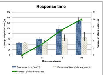
0! 2! 4! 6! 8! 10! 12! 0! 20! 40! 60! 80! 100! 120! 140! 160! 4! 8! 12! 16! N u m b e r o f c lo u d i n s ta n c e s ! A v e ra g e r e s p o n s e ti m e (s ) ! Concurrent users! Response time!

Response time (static)! Response time (static + dynamic)!

Number of cloud instances!

Figure 2: Average response time for concurrent re-quests on large input files

machine on the Internet with a latency distance of approxi-mately 150 ms to the Alamo cloud. For our experiments we bypassed the CyberGIS Gateway and the GISolve middle-ware and configured JMeter to interact directly with HAProxy. This approach allowed us to use the WPS interface of the spatial regression service directly, which simplifies the script-ing of the requests.

Each experiment was run only once. We averaged the response time of all the requests during one experiment to produce the results and also display the standard deviation of the response time as error bars.

While the service interface does not impose any restric-tions on the locarestric-tions of input data, in the interest of sim-plicity here we assumed that the input files are hosted on the data store server.

4.1 Large Requests

In our first experiment, we use a scenario representing scientists using the CyberGIS platform as part of their re-search work. These users work on a small number of files with large sizes. The scientists make regular requests with different settings in order to explore the correlations in their data sets. We simulate this scenario with the following con-ditions. Each user performs 5 requests for spatial regression on a data file with 1,000,000 entries and 9 variables. Each user pauses 10 seconds between the requests (time to change the settings). We vary the number of users concurrently ac-cessing the platform from 8 to 16. We configured Apache JMeter to use a ramp-up period of 30 seconds, in order to add variability to the arrival time of the requests. We use a static virtual cluster of 5 instances. We set a maximum of 10 dynamic cloud instances. We keep a request history of 2 minutes.

In this experiment, each instance is set up to process only one concurrent request, since requests on large files require a lot of resources and several concurrent large requests on the same machine can lead to errors due to free memory shortage.

Figure 2 shows the average response time experienced by users in two scenarios: the first (blue) with a service served by a static virtual cluster of 5 instances, and the second (red) with the static virtual cluster augmented with instances

(6)

0 2 4 6 8 10 12 14 16 18 0 100 200 300 400 500 600 0 2 4 6 8 10 12 14 16 18

Number of connections Number of instances

Time (s) Impact of concurrent requests

Number of connections Dynamic cloud instances Total instances

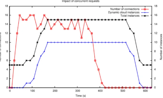
Figure 3: Impact of concurrent requests

namically provisioned from the cloud. The figure shows that while the average latency increases steadily in the static vir-tual cluster, our auto-scaling architecture handles the in-creasing load more efficiently by provisioning a proportional number of cloud instances dynamically. In this case, our system deploys enough instances (green line) to have each concurrent user handled by a separate instance.

To better analyze what happens when extending the static resources dynamically with cloud instances, we show in Fig-ure 3 the number of requests to the system and the number of active instances (both the number of dynamic cloud in-stances and the total number of inin-stances) in the previous experiment with 16 concurrent users. We observe that as the number of requests gets to 16, the number of dynamic cloud instances increases shortly after. The lag between the increase in the number of requests and the increase in ac-tive instances is explained by the time taken by the cloud to provision instances. The number of dynamic cloud in-stances peaks at 10, since this is the maximum that we have set. Without this limit it would peak at 11 (16 concurrent requests minus 5 static VMs).

In Figure 4, we show how those extra instances help re-duce the response time for users. Each red bar corresponds to the response time of a separate request. We see that the first group of 16 requests at the beginning of the exper-iment is answered with increasing response time: the first requests are answered in between 40 to 50 seconds, while the slowest response takes close to 150 seconds. However, this heavy load on our five static instances causes extra cloud instances to be provisioned dynamically. We then observe that the response time decreases as more instances become available, and stabilizes back around 40 to 50 seconds. The high response time at the beginning of the experiment ex-plains why Figure 2 shows a higher response time for 16 concurrent users than for 8, even though once enough in-stances are provisioned, the same response time should be provided.

4.2 Small Files

Our second set of experiment corresponds to a scenario where a classroom of students are attending a CyberGIS tu-torial. As they follow the instructions of the tutorial, a large number of students make repeated requests to the service. These requests use small files, since students normally do not need large data sets to learn the software. We simulate this scenario with the following conditions. Each student

0 20 40 60 80 100 120 140 160 0 100 200 300 400 500 600 0 5 10 15 20

Response time (s) _{Number of instances}

Time (s)

Impact of dynamic cloud instances over response time

Response time Dynamic cloud instances Total instances

Figure 4: Impact of dynamically adding cloud in-stances over response time

0! 1! 2! 3! 4! 5! 6! 7! 8! 0! 20! 40! 60! 80! 100! 120! 140! 160! 32! 48! 64! N u m b e r o f c lo u d i n s ta n c e s ! A v e ra g e r e s p o n s e ti m e (s ) ! Concurrent users! Response time!

Response time (static)! Response time (static + dynamic)!

Number of cloud instances!

Figure 5: Average response time for the student

tutorial use case

performs five requests for spatial regression on a small data file. Each student pauses 10 seconds between requests (time to change the settings). We vary the number of students concurrently accessing the platform from 32 to 64. We use a single instance for the static resources. We set a maximum of 10 dynamic cloud instances. We keep a request history of 2 minutes.

In this experiment, the maximum number of requests per instance is set to 8. Requests on these small files are less resource intensive than in the previous experiment; hence, several requests can be scheduled concurrently on the same VM. We set the maximum number of cloud instances to 10 (in addition to the existing static instance).

Figure 5 shows the average response time of requests for various number of students (32, 48, and 64). The error bars represent the standard deviation of the response time. We can clearly see that the average response time rises signifi-cantly when using a single static VM: from 62.5 seconds for 32 students up to more than two minutes for 64 students, an increase of more than 113%. In comparison, the response time when using cloud instances is lower (23 seconds for 32 users) and rises more slowly (29.5 seconds for 64 students, an increase of less than 30%). As in the previous experi-ment, the number of cloud instances increases linearly with the number of concurrent users.

(7)

5. USE CASE ANALYSIS

The spatial regression application accessible through the CyberGIS Gateway is open for access to the spatial econo-metrics community and other CyberGIS user communities. The typical usage models of the application on the Gateway correspond well with the two scenarios (large data analysis, large number of analysis) that were studied in Section 4. The auto-scaling approach achieved through the integration with the Nimbus Phantom cloud platform plays the key role in satisfying the demanding responsiveness requirements of these scenarios that conventional job-queue-based comput-ing model was not able to meet. Compared with the original solution that dedicated a static virtual cluster for the analy-sis, the modified auto-scaling based cloud computing model has the advantage of leveraging a large amount of cloud com-puting resources in an on-demand fashion. In fact, through our experiments we have shown the modified solution lever-aging auto-scaling is well positioned to meet the computa-tional and scalabilities requirements posed by both usage models.

Encouraged by this study we are investigating how to use the auto-scaling cloud platform to integrate other Cyber-GIS analytics with interactive requirements (e.g., FluMap-per [21]) or other response time requirements (e.g., appli-cations with sporadic high-load access from classroom) and are also compute-intensive and/or data-intensive. Accord-ingly, we have identified additional features that our ap-proach needs to support: in particular data models that can use cloud-provided storage to persist across the lives of VM instances as well as scale to feed potentially large numbers of VMs. Additionally, we will study further how our sys-tem can dynamically adapt to variable request sizes, so that a mix of requests can be handled exploring optimal assign-ments to resources at job or load balancer level. On the resource management level we seek to make the response times more reliable and uniform so that they can be repre-sented as a true quality of service; this can be achieved via approaches based on pre-deployment and prediction as e.g. in [19], as well as coordination of multiple resources includ-ing storage and networkinclud-ing. Finally, last on our wishlist is correlating the response time to the cost aspects of our ser-vice: while our initial implementation ran on FutureGrid it is likely that future deployments will use a range of private and commercial clouds and thus leveraging results like [17] will have increased significance.

6. CONCLUDING DISCUSSION

In this paper, we presented our work on extending the architecture of CyberGIS to dynamically add on-demand cloud resources in order to improve the responsiveness of spatial data analysis and highlight the parts of the system that had to be adapted to achieve this goal. We implemented our solution in the context of the CGPySAL application, which gives access to PySAL spatial regression modeling for spatial econometrics analysis. Our experiments, performed on a FutureGrid cloud, show that our system can automati-cally react to changes in the number of user requests and can provision additional cloud resources accordingly. This allows the response time to remain low with a growing number of requests, which is crucial for maintaining the responsiveness requirements of CyberGIS. While our solution shows good scalability in two separate use cases using different compute

node configurations, we will need to investigate further how to dynamically and economically support variable request sizes. Although we did not encounter data-related limita-tions in our evaluation, we will also investigate how our sys-tem can scale the data storage backend in order to support rapidly the growing sizes of spatial data sets.

7. ACKNOWLEDGMENTS

This work was supported by the U.S. Department of En-ergy, Office of Science, under Contract DE-AC02-06CH11357. This material is also based in part upon work supported by the National Science Foundation under the grant number: 1047916. Any opinions, findings, and conclusions or recom-mendations expressed in this material are those of the au-thors and do not necessarily reflect the views of the National Science Foundation.

8. REFERENCES

[1] L. Anselin, P. V. Amaral, and D. Arribas-Bel. Technical Aspects of Implementing GMM Estimation of the Spatial Error Model in PySAL and

GeoDaSpace.

http://geodacenter.asu.edu/drupal files/sperrorgmm wp2.pdf, 2012.

[2] L. Anselin and S. J. Rey. Spatial Econometrics in an Age of CyberGIScience.International Journal of Geographical Information Science, 26(12):2211–2226, Dec. 2012.

[3] Apache Software Foundation. Apache JMeter. https://jmeter.apache.org, 2014.

[4] M. Armbrust, A. Fox, R. Griffith, A. D. Joseph, R. H. Katz, A. Konwinski, G. Lee, D. A. Patterson,

A. Rabkin, I. Stoica, and M. Zaharia. Above the Clouds: A Berkeley View of Cloud Computing. Technical report, University of California at Berkeley, Feb. 2009.

[5] J. Arrigo, D. Tarboton, and A. Couch. Building and Sustaining Community Cyber-Infrastructure for the Hydrologic Sciences.Eos, Transactions American Geophysical Union, 94(47):435–435, 2013. [6] B. Baranski, B. Sch¨affer, and R. Redweik.

Geoprocessing in the Clouds.Journal of the Open Source Geospatial Foundation, 8:17–22, Feb. 2011. [7] B. Behzad, A. Padmanabhan, Y. Liu, Y. Liu, and

S. Wang. Integrating CyberGIS Gateway with Windows Azure: A Case Study on MODFLOW Groundwater Simulation. InProceedings of the ACM SIGSPATIAL Second International Workshop on High Performance and Distributed Geographic Information Systems, HPDGIS ’11, pages 26–29, 2011.

[8] J. D. Blower. GIS in the Cloud: Implementing a Web Map Service on Google App Engine. InProceedings of the 1st International Conference and Exhibition on Computing for Geospatial Research & Application, COM.Geo ’10, pages 34:1–34:4, 2010.

[9] G. J. Bowen, J. B. West, L. Zhao, G. Takahashi, C. Miller, and T. Zhang. Cyberinfrastructure for isotope analysis and modeling.Eos, Transactions American Geophysical Union, 93(19):185–187, 2012. [10] B. A. Bryan. High-performance computing tools for

(8)

social-ecological systems.Environmental Modelling & Software, 39:295–303, Jan. 2013.

[11] C. Flores. haproxyctl.

https://github.com/flores/haproxyctl.

[12] J. Gong, P. Yue, and H. Zhou. Geoprocessing in the Microsoft cloud computing platform – Azure. InA special joint symposium of ISPRS Technical Commission IV & AutoCarto in conjunction with ASPRS/CaGIS 2010 Fall Specialty Conference, 2010. [13] Q. Huang, C. Yang, D. Nebert, K. Liu, and H. Wu.

Cloud Computing for Geosciences: Deployment of GEOSS Clearinghouse on Amazon’s EC2. In

Proceedings of the ACM SIGSPATIAL International Workshop on High Performance and Distributed Geographic Information Systems, pages 35–38, 2010. [14] K. Keahey, P. Armstrong, J. Bresnahan,

D. LaBissoniere, and P. Riteau. Infrastructure Outsourcing in Multi-cloud Environment. In

Proceedings of the 2012 Workshop on Cloud Services, Federation, and the 8th Open Cirrus Summit, FederatedClouds ’12, pages 33–38, 2012.

[15] C. Kiehle, K. Greve, and C. Heier. Requirements for Next Generation Spatial Data

Infrastructures-Standardized Web Based Geoprocessing and Web Service Orchestration.

Transactions in GIS, 11(6):819–834, 2007.

[16] T. Lorido-Botr´an, J. Miguel-Alonso, and J. A. Lozano. Auto-scaling Techniques for Elastic Applications in Cloud Environments. Technical Report EHU-KAT-IK, Department of Computer Architecture and

Technology, UPV/EHU, 2012.

[17] M. Mao and M. Humphrey. Auto-scaling to Minimize Cost and Meet Application Deadlines in Cloud Workflows. InProceedings of 2011 International Conference for High Performance Computing, Networking, Storage and Analysis, SC ’11, pages 49:1–49:12, 2011.

[18] P. Mell and T. Grance. The NIST Definition of Cloud Computing. Technical Report 800-145, National Institute of Standards and Technology (NIST), Sept. 2011.

[19] B. Nicolae, P. Riteau, and K. Keahey. Bursting the Cloud Data Bubble: Towards Transparent Storage Elasticity in IaaS Clouds. In28th IEEE International Parallel & Distributed Processing Symposium, 2014. [20] T. L. Nyerges, M. J. Roderick, and M. Avraam.

CyberGIS Design Considerations for Structured Participation in Collaborative Problem Solving.

International Journal of Geographical Information Science, 27(11):2146–2159, Nov. 2013.

[21] A. Padmanabhan, S. Wang, G. Cao, M. Hwang, Y. Zhao, Z. Zhang, and Y. Gao. FluMapper: An Interactive CyberGIS Environment for Massive Location-based Social Media Data Analysis. In

Proceedings of the Conference on Extreme Science and Engineering Discovery Environment: Gateway to Discovery, XSEDE ’13, pages 33:1–33:2, 2013. [22] S. J. Rey and L. Anselin. PySAL: A Python Library

of Spatial Analytical Methods.The Review of Regional Studies, 37(1), 2007.

[23] J. L. Schnase, D. Q. Duffy, G. S. Tamkin, D. Nadeau, J. H. Thompson, C. M. Grieg, M. A. McInerney, and

W. P. Webster. MERRA analytic services: Meeting the big data challenges of climate science through cloud-enabled climate analytics-as-a-service.

Computers, Environment and Urban Systems, 2014. [24] Y. Shao, L. Di, Y. Bai, B. Guo, and J. Gong.

Geoprocessing on the Amazon cloud computing platform – AWS. InFirst International Conference on Agro-Geoinformatics, pages 1–6, Aug. 2012.

[25] W. Tarreau. HAProxy: The Reliable, High Performance TCP/HTTP Load Balancer. http://haproxy.1wt.eu/.

[26] The Nimbus Project. Building a Decision Engine with the Phantom Scripting API.

http://www.nimbusproject.org/phantom. [27] The Nimbus Project. Nimbus Phantom.

http://www.nimbusproject.org/phantom.

[28] S. Wang. A CyberGIS Framework for the Synthesis of Cyberinfrastructure, GIS, and Spatial Analysis.

Annals of the Association of American Geographers, 100:535–557, 2010.

[29] S. Wang, L. Anselin, B. Bhaduri, C. Crosby, M. F. Goodchild, Y. Liu, and T. L. Nyerges. CyberGIS Software: A Synthetic Review and Integration Roadmap.International Journal of Geographical Information Science, 27(11):2122–2145, Nov. 2013. [30] S. Wang, M. Armstrong, J. Ni, and Y. Liu. GISolve: a

grid-based problem solving environment for computationally intensive geographic information analysis. InChallenges of Large Applications in Distributed Environments, 2005. CLADE 2005. Proceedings, pages 3–12, July 2005.

[31] S. Wang and Y. Liu. TeraGrid GIScience Gateway: Bridging Cyberinfrastructure and GIScience.

International Journal of Geographical Information Science, 23(5):631–656, May 2009.

[32] S. Wang, N. Wilkins-Diehr, and T. L. Nyerges. CyberGIS – Toward synergistic advancement of cyberinfrastructure and GIScience: A workshop summary.Journal of Spatial Information Science, 4(1):125–148, 2012.

[33] S. Wang and X.-G. Zhu. Coupling Cyberinfrastructure and Geographic Information Systems to Empower Ecological and Environmental Research.BioScience, 58:94–95, 2008.

[34] C. Yang, M. Goodchild, Q. Huang, D. Nebert, R. Raskin, Y. Xu, M. Bambacus, and D. Fay. Spatial cloud computing: how can the geospatial sciences use and help shape cloud computing? International Journal of Digital Earth, 4(4):305–329, 2011. [35] L. Yin, S.-L. Shaw, D. Wang, E. A. Carr, M. W.

Berry, L. J. Gross, and E. J. Comiskey. A framework of integrating GIS and parallel computing for spatial control problems – a case study of wildfire control.

International Journal of Geographical Information Science, 26(4):621–641, 2012.

[36] Y. Zhong, J. Han, T. Zhang, and J. Fang. A distributed geospatial data storage and processing framework for large-scale WebGIS. In2012 20th International Conference on Geoinformatics (GEOINFORMATICS), pages 1–7, June 2012.

A Cloud Computing Approach to On-Demand and Scalable CyberGIS Analytics