Evolutionary Search Techniques with Strong Heuristics for
Evolutionary Search Techniques with Strong Heuristics for
Multi-Objective Feature Selection in Software Product Lines
Objective Feature Selection in Software Product Lines
Abdel Salam SayyadWest Virginia University
Follow this and additional works at: https://researchrepository.wvu.edu/etd Recommended Citation
Recommended Citation
Sayyad, Abdel Salam, "Evolutionary Search Techniques with Strong Heuristics for Multi-Objective Feature Selection in Software Product Lines" (2014). Graduate Theses, Dissertations, and Problem Reports. 303. https://researchrepository.wvu.edu/etd/303
This Dissertation is protected by copyright and/or related rights. It has been brought to you by the The Research Repository @ WVU with permission from the rights-holder(s). You are free to use this Dissertation in any way that is permitted by the copyright and related rights legislation that applies to your use. For other uses you must obtain permission from the rights-holder(s) directly, unless additional rights are indicated by a Creative Commons license in the record and/ or on the work itself. This Dissertation has been accepted for inclusion in WVU Graduate Theses, Dissertations, and Problem Reports collection by an authorized administrator of The Research Repository @ WVU. For more information, please contact [email protected].
Evolutionary Search Techniques with Strong Heuristics for Multi-Objective Feature Selection in Software Product Lines
by
Abdel Salam Sayyad Dissertation Submitted to
the Benjamin M. Statler College of Engineering and Mineral Resources at West Virginia University
in Partial Fulfillment of the Requirements for the Degree of
Doctor of Philosophy In
Computer Engineering Approved by:
Dr. Hany Ammar, Committee Chair Dr. Tim Menzies, Committee co-Chair Dr. Ramana Reddy
Dr. Ali Mili
Dr. Mario Perhinschi
Lane Department of Computer Science and Electrical Engineering Morgantown, WV, USA
August 2014
Keywords: Software Product Lines, Metaheuristic Search Algorithms, Multi-Objective Optimization, Search-Based Software Engineering
Evolutionary Search Techniques with Strong Heuristics for Multi-Objective Feature Selection in Software Product Lines
Abdel Salam Sayyad
Software design is a process of trading off competing objectives. If the user objective space is rich, then we should use optimizers that can fully exploit that richness. For example, this study configures software product lines (expressed as feature models) using various search-based software engineering methods. Our main result is that as we increase the number of optimization objectives, the methods in widespread use (e.g. NSGA-II, SPEA2) perform much worse than IBEA (Indicator-Based Evolutionary Algorithm). IBEA works best since it makes most use of user preference knowledge. Hence it does better on the standard measures (hypervolume and spread) but it also generates far more products with 0 violations of domain constraints. We also present significant improvements to IBEA’s performance by employing three strong heuristic techniques that we call PUSH, PULL, and seeding. The PUSH technique forces the evolutionary search to respect certain rules and dependencies defined by the feature models, while the PULL technique gives higher weight to constraint satisfaction as an optimization objective and thus achieves a higher percentage of fully-compliant configurations within shorter runtimes. The seeding technique helps in guiding very large feature models to correct configurations very early in the optimization process. Our conclusion is that the methods we apply in search-based software engineering need to be carefully chosen, particularly when studying complex decision spaces with many optimization objectives. Also, we conclude that search methods must be customized to fit the problem at hand. Specifically, the evolutionary search must respect domain constraints.
My deepest thanks and appreciation go to my PhD advisors: Prof. Hany Ammar and Prof. Tim Menzies, for their immense guidance and endless support.
This research work was funded by the Qatar National Research Fund (QNRF) under the National Priorities Research Program (NPRP) Grant No.: 09-1205-2-470, and the National Science Foundation (NSF) Grant No.: CCF 1017330.
i
List of Tables ...v
List of Figures ... vi
List of Acronyms ... viii
Chapter 1: Introduction to the Study ...1
1.1 Contributions of This Work ...5
1.2 Published Results ...6
1.3 Recent Results ...7
1.4 Statement of Thesis ...8
1.5 Organization of This Document ...9
Chapter 2: Background ...10
2.1 Software Product Line Engineering (SPLE) ...10
2.2 Feature Models...10
2.3 Tools for Automated Analysis of Feature Models ...14
2.3.1 Binary Decision Diagrams (BDD) ... 15
2.3.2 The Satisfiability (SAT) Problem ... 15
2.3.3 The Constraint Satisfaction Problem (CSP) ... 16
2.3.4 Satisfiability Modulo Theories (SMT)... 16
2.3.5 The Infeasibility of Exhaustive Search for Optimal Configuration ... 17
2.4 Genetic Algorithm ...18
2.5 Multi-Objective Evolutionary Algorithms (MOEAs) ...19
ii
2.8 Summary ...24
Chapter 3: Problem Formulation ...25
3.1 Problem Definition...25
3.2 Extending Feature Models with Attributes ...25
3.3 Our Approach to Assigning Feature Attributes ...26
3.4 Defining the Optimization Objectives ...27
3.5 Why Maximize the Number of Features? ...27
3.6 Quality of Pareto Front ...28
3.7 Run Time versus Number of Evaluations; Which One Shall Be Fixed? ...29
3.8 Relationship with Interactive Configuration ...31
Chapter 4: Related Work ...32
4.1 Automated Analysis of Feature Models ...32
4.2 Optimizing Feature Models with Attributes ...34
4.3 Pareto-Optimal Search-Based Software Engineering ...36
4.3.1 Algorithms ... 42
4.3.2 Number of Objectives ... 44
4.3.3 Tools/Frameworks ... 45
4.3.4 Quality Indicators... 45
4.3.5 Survey Summary ... 46
Chapter 5: Experimental Setup ...48
iii
5.3 Algorithm Implementation...49
5.4 Strong Heuristics to Improve Performance ...50
5.4.1 The PUSH Technique ... 50
5.4.2 The PULL Technique ... 51
5.4.3 Population Seeding ... 52
Chapter 6: Results ...53
6.1 Increasing the Number of Optimization Objectives ...53
6.2 Parameter Tuning ...57
6.3 Using Strong Heuristics: PUSH and PULL ...63
6.4 Objective Development over Time ...70
6.5 Population Seeding ...72
6.5.1 Parameter Settings ... 74
6.5.2 Method for Generating a Correct Seed ... 75
6.5.3 Result of Using PUSH and Seeding (no PULL) ... 75
6.5.4 Result of Using PUSH, PULL, and Seeding... 77
6.5.5 Investigating the Diversity of Solutions Achieved with Seeding ... 79
Chapter 7: Threats to Validity ...85
7.1 Threats to Construct Validity ...85
7.1.1 Sampling Bias ... 85
7.1.2 Treatment Bias ... 86
iv
7.2 Threats to Internal Validity ...88
7.3 Threats to Conclusion Validity ...88
7.4 Threats to External Validity ...89
Chapter 8: Discussion ...90
8.1 Method for Achieving Correct Configurations ...90
8.2 Indicator-Based Evolutionary Algorithm (IBEA) vs. Other MOEAs ...90
8.3 Run Time Improvements ...92
8.4 Potential for “User-In-The-Loop” Design ...92
Chapter 9: Conclusions and Future Work ...94
9.1 Conclusions ...94
9.2 Future Work ...95
References ...99
v
Table 1: Sample attributes added to feature models ... 26
Table 2: List of surveyed Pareto-Optimal SBSE works in software requirements... 38
Table 3: List of surveyed Pareto-Optimal SBSE works in software design ... 39
Table 4: List of surveyed Pareto-Optimal SBSE works in software testing ... 40
Table 5: List of surveyed Pareto-Optimal SBSE works in project management ... 41
Table 6: SPLOT feature models used in the study ... 48
Table 7: LVAT feature models used in the study ... 49
Table 8: Fixed features and skipped rules for LVAT models ... 52
Table 9: Parameter settings for first experiment ... 53
Table 10: Comparison of quality indicators, 2 and 3 objectives... 55
Table 11: Comparison of quality indicators, 4 and 5 objectives... 55
Table 12: Various runs with IBEA on E-Shop, 5 objectives ... 56
Table 13: Experimental setup for parameter tuning ... 58
Table 14: Summary of parameter tuning results ... 61
Table 15: Parameter settings used for experiment with PUSH and PULL ... 63
Table 16: Results of 5-objective optimization; PUSH without PULL ... 64
Table 17: Results of 5-objective optimization; PUSH and PULL ... 67
Table 18: Parameter settings for seeding experiment ... 74
Table 19: Time and number of selected features for generated seed ... 75
vi
Figure 1: Feature model for mobile phone product line, adopted from [3] ... 11
Figure 2: Mobile phone feature model in SXFM format ... 12
Figure 3: Mobile phone feature model as a Boolean expression ... 13
Figure 4: Example Binary Decision Diagram ... 15
Figure 5: Genetic Algorithm, adapted from [22] ... 18
Figure 6: Example of a single-point crossover, from [22] ... 19
Figure 7: Indicator-Based Evolutionary Algorithm (IBEA) ... 21
Figure 8: NSGA-II sorting procedure, from [13]... 22
Figure 9: Pareto-Optimal SBSE papers by area of application ... 37
Figure 10: Pareto-Optmal SBSE papers by publication year... 37
Figure 11: Pareto-Optimal SBSE algorithms by frequency of use ... 42
Figure 12: Pareto-Optimal SBSE algorithms by frequency of use (single-algo. papers) . 43 Figure 13: Reasons for adopting an algorithm in Pareto-Optimal SBSE ... 44
Figure 14: Number of objectives by frequency of use in Pareto-Optimal SBSE ... 45
Figure 15: Tree mutation procedure ... 50
Figure 16: Comparison of TT100% for IBEA with and without the PULL method ... 69
Figure 17: Development of quality indicators over time for E-Shopping ... 71
Figure 18: Development of normalized mean values over time for E-Shopping ... 71
Figure 19: Development of quality indicators over time for uClinux ... 73
Figure 20: Development of normalized mean values over time for uClinux ... 73
vii
Figure 23: Box plot against time for the number of selected features. ... 80
Figure 24: Box plot against time for the number of features used before. ... 81
Figure 25: Box plot against time for the number of known defects. ... 82
viii BDD Binary Decision Diagram
CSP Constraint Satisfaction Problem CTC Cross-Tree Constraint
DIMACS Discrete Mathematics and Theoretical Computer Science FastPGA Fast Pareto Genetic Algorithm
HV Hypervolume
IBEA Indicator-Based Evolutionary Algorithm LVAT Linux Variability Analysis Tools
MOCell Multi-Objective Cellular Genetic Algorithm MOEA Multi-Objective Evolutionary Algorithm NSGA Nondominated Sorting Genetic Algorithm
POSBSE Pareto-Optimal Search-Based Software Engineering SAT The Satisfiability Problem
SBSE Search-Based Software Engineering SMT Satisfiability Modulo Theories
SPEA Strength Pareto Evolutionary Algorithm SPL Software Product Line
SPLE Software Product Line Engineering SPLOT Software Product Line Online Tools
Chapter 1: Introduction to the Study
Software engineering technologies are increasingly having a direct impact on business outcomes, so much so that software decisions must be value-driven early on, i.e. business concerns ought to play a central role in the selection of software tools, technologies and processes. Barry Boehm states that: “software has a major influence on most systems’ cost, schedule, and value; and value-neutral software decisions can seriously degrade project outcomes.” [16] This comment is most relevant to the subject of this thesis, in which we choose our evolutionary optimization algorithm to best exploit the user preferences in search for optimized feature selections in a software product line (SPL). This problem entails searching the space of possible feature configurations for sets of feature selections that conform to domain constraints, but another goal is to increasingly optimize the objectives that the user cares about, such as cost and reliability metrics.
The global information technology infrastructure is becoming increasingly reliant on increasingly complex software. This study is about the way to rapidly explore and configure such complexity. Feature models allow visualization, reasoning, and configuration of large and complex software product lines (SPLs). Common SPLs now consist of hundreds (even thousands) of features, with complex dependencies and constraints that govern which features can or cannot live and interact with other features. For instance, according to [14], the Linux model has 6320 features, of which 86% declare
constraints of some sort, and most features refer to 2-4 other features. Such level of complexity surely requires automated reasoning and configuration techniques, especially if the intricacies of the feature model are combined with further user preferences and priorities, such as those related to cost and reliability. In that case, the job of offering product variants with guaranteed conformance to the feature model and efficiency according to user preferences becomes monumental, requiring tool assistance.
Many Search-Based Software Engineering (SBSE) researchers who seek to apply metaheuristic search methods to their problems choose the algorithms based on popularity of the algorithm in the SE literature, or its wide usage in other fields. Harman makes the following comment regarding the choice of evolutionary search algorithms over non-evolutionary ones: “We must be wary of the unquestioning adoption of evolutionary algorithms merely because they are popular and widely applicable or because, historically, other researchers have adopted them for SBSE problems; none of these are scientific motivations for adoption.” [46] We believe the same comment applies to choosing certain evolutionary algorithms over others.
Most importantly, the chosen algorithms have to accommodate both the user preferences and the structure of the decision space. In [86] and [85], we use IBEA (Indicator-Based Evolutionary Algorithm) to best exploit user preference knowledge, but the search takes hours to produce a significant amount of model-conforming solutions. In more recent results, we quickly achieve 100% fully-conformant solutions, and the remaining time is spent on further optimizing solutions according to user preferences. We
accomplish this remarkable gain by introducing three strong heuristic techniques: PUSH, PULL, and population seeding. The PUSH technique first learns certain rules from static analysis of the feature model, and then forces the evolutionary process to respect those rules. The PULL technique gives more weight to constraint satisfaction in the optimization process, and thus achieves full conformance in all solutions within shorter time. The seeding technique pre-computes one valid configuration and then implants it in the initial population as a model for the other individuals to follow, which helps find many good solutions sooner in many-objective optimization of feature models with thousands of features and hundreds of thousands of constraints. We demonstrate the usefulness of our methods by optimizing the configuration of 20 medium-sized academic feature models from the SPLOT repository (Software Product Line Online Tools)1, in addition to 7 large real feature models from the LVAT repository (Linux Variability Analysis Tools)2.
The scalability of our results to large feature models derived from actual software systems (LVAT) is of significant importance. Scalability of SBSE methods can mean the difference between theoretical obscurity and industrial adoption. The larger and more complex the application examples are, the closer they resemble practical applications, and the more believable the result will be. Yet the lack of scalability of results is one of the biggest problems facing software engineers, according to Harman et al. [50]. They
1
http://www.splot-research.org
state that: “Many approaches that are attractive and elegant in the laboratory turn out to be inapplicable in the field, because they lack scalability.”
A case in point is the subject of this paper: the many-objective optimum feature selection in software product lines. Many results in the automated analysis of software product lines were validated using feature models published in online feature model repositories such as SPLOT [68]. Examples are: Pohl et al. [75], Lopez-Herrejon and Egyed [64], Johansen et al. [55], Mendonca et al. [70] and our own previous work [86], [84]. Most of the feature models in SPLOT were produced for academic purposes without representing actual systems. One such model is “Electronic Shopping,” designed by Lau [62], the largest in SPLOT with 290 features. While it might be a “best effort” in emulating a real system, it does not represent an actual project. Berger et al. [15] explain in detail the differences in properties between SPLOT feature models and the large feature models that they developed by reverse-engineering real systems, and published in the LVAT (Linux Variability Analysis Tools) repository. In short, SPLOT models had significantly smaller and less constrained models with lower branching factors, but they also had higher ratios of feature groups and deeper leaves than LVAT models. This shows an underlying gap between academic assumptions and actual properties of software product lines.
The only two studies we know that experimented with the LVAT feature models were done by Johansen et al. [55] who generated test covering arrays for feature models, and Henard et al. [54] who worked on prioritizing t-wise test suites. Both experimented
with three very large models from the LVAT repository (Linux, eCos, and FreeBSD), in addition to models from SPLOT and other sources. Our work is the first to attempt the many objective optimization of product line configuration.
Other researchers attempted to prove scalability of their methods using randomly-generated feature models that followed a set of assumed characteristics. Examples are: White et al. [105] [104] [103] [106], Shi et al. [88], Guo et al. [45], and Mendonca et al. [70]. While those randomly-generated models can be larger in size than published models, they still suffer from the same assumptions that diverge from the properties of real systems.
1.1 Contributions of This Work
The overall contributions of our work in optimum feature selection in software product lines are summarized as follows:
1- The formulation of this problem as a multi-objective optimization problem which requires a Pareto-efficient set of solutions. Although related work (see section 3.2) also defined secondary objectives in feature model configuration, they aggregated the multiple objectives into a single fitness function, and searched for a single optimum solution, which is of less benefit to the end user.
2- We use Multi-Objective Evolutionary Algorithms (MOEAs) for the first time to provide solutions for this problem, and comparing the performance of multiple MOEAs based on quality indicators and the amount of solutions that conform to the feature models. We demonstrate the remarkable advantage of the Indicator-Bases
Evolutionary Algorithm (IBEA). Wagner et al. [98] show that Indicator-Based algorithms (such as IBEA) perform remarkably better than Pareto-Based algorithms (such as NSGA-II) when applied to many-objective problems. Our research was the first to confirm that result in software engineering.
3- We validate our results using 20 medium-sized feature models developed as academic examples and 7 large feature models that were reverse-engineered from actual projects. The total number of features ranged between 43 and 6888 features.
4- We achieve fast run times which allow the practical use of IBEA in interactive configuration of feature models. Within 1 second, we are able to provide the user with a wide range of model-conforming solutions. This is possible with the help of the PUSH and PULL techniques, and with better-tuned evolutionary parameters.
5- A breakthrough scalability result. Using the population seeding technique we now show that it is possible to configure product lines as large as 6000+ features, and 344,000 constraints.
1.2 Published Results
In our earliest work [86] we tackled the problem of configuring software product lines as a high-dimensional multi-objective search problem, and we compared Pareto-optimal solutions from several algorithms to show the superiority of IBEA. In that paper, we only used two feature models, and we experienced long run times which can only correspond with offline optimization.
In [84] and [83], we improved the performance of IBEA with regard to configuration of feature models by reducing the rates of crossover and mutation. We found that the “rule-of-thumb” rates often used with evolutionary algorithms amount to lengthening the duration of the search. This highlights the fine-grained structure of the feature models, where small changes in features have great effects on other features, and thus the search needs to proceed slowly for better exploration of the decision space.
In [85], we compare the performance of IBEA against NSGA-II when applied to large feature models from the LVAT (Linux Tools) repository. We utilize “feature fixing” as a way to force the search to respect certain rules that we learn from the feature models. We also report on an early result using the “population seeding” heuristic, which we expand in this document.
1.3 Recent Results
Here, we introduce the “Tree Mutation” operator which only mutates (flips) a feature selection decision if that mutation is allowed by the tree structure, i.e. the mutation is not allowed to override parent-child dependencies or group selection restrictions. Tree mutation is only applied to SPLOT models since they explicitly represent the feature tree. For LVAT models, we employ “feature fixing” which was introduced in [85]. Together, “tree mutation” and “feature fixing” are called the PUSH technique in this paper; since they both restrict the evolutionary process using pre-learned knowledge about feature model structure.
We also introduce the PULL technique, which give more weight to constraint violation as a minimization objective; thus achieving significant amounts of model-conforming configurations sooner and accelerating the multi-objective search. Together, the PUSH and PULL techniques achieve runtime improvement of over 16,000 times for the E-Shopping feature model than achieved in [86].
We present the results of an extensive experiment comparing five different algorithms applied to 27 software product lines. IBEA with PUSH and PULL emerged, as expected, as the ultimate optimization tool with regard to the configuration of hierarchically-modeled software systems.
1.4 Statement of Thesis
We propose that the optimizers we choose must be considered according to the nature of the problem at hand; for example, when the user preference space is rich, choose an optimizer that exploits that richness. In particular, we find that an optimizer which uses continuous dominance for its fitness raking is better at many-objective optimization than those depending on Boolean dominance.
In addition, we advocate the customization of our optimizers to the problem domain such that it searches for solutions while respecting domain constraints. This calls for the deployment of strong heuristics which guide the search algorithm into promoting solutions that are close to domain conformance; rather than spending search and evaluation time on less conforming solutions.
1.5 Organization of This Document
The rest of this document is organized as follows: Chapter 2 provides background material on software product lines, genetic algorithms, and MOEAs. Chapter 3 introduces the problem formulation. Chapter 4 reviews related work in the use of MOEAs in software engineering. Chapter 5 describes the experimental setup, and chapter 6 presents the experimental results. Chapter 7 presents the threats to validity. In chapter 8, we discuss our findings and their implications. Finally, chapter 9 presents conclusions and future work.
Chapter 2: Background
2.1 Software Product Line Engineering (SPLE)
Increasingly, software engineers spend their time creating software families consisting of similar systems with many variations [26]. Many researchers in industry and academia started using a feature-oriented approach to commonality and variability analysis after the Software Engineering Institute introduced Feature-Oriented Domain Analysis (FODA) in 1990 [56]. Software product line engineering is a paradigm to develop software applications using platforms and mass customization. Benefits of SPLE include reduction of development costs, enhancement of quality, reduction of time to market, reduction of maintenance effort, coping with evolution and complexity [74], and identifying opportunities for automating the creation of family members [26].
2.2 Feature Models
A feature is an end-user-visible behavior of a software product that is of interest to some stakeholder. A feature model represents the information of all possible products of a software product line in terms of features and relationships among them. Feature models are a special type of information model widely used in software product line engineering. A feature model is represented as a hierarchically arranged set of features composed by:
1. Relationships between a parent feature and its child features (or subfeatures).
2. Cross-tree constraints that are typically inclusion or exclusion statements in the form: if feature F is included, then features A and B must also be included (or excluded).
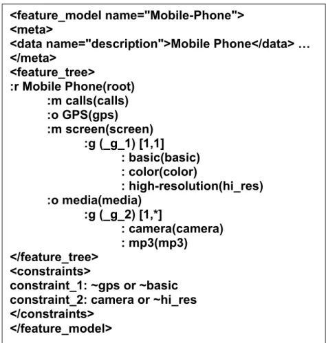
Figure 1, adapted from [11], depicts a simplified feature model inspired by the mobile phone industry.
<feature_model name="Mobile-Phone"> <meta>
<data name="description">Mobile Phone</data> … </meta> <feature_tree> :r Mobile Phone(root) :m calls(calls) :o GPS(gps) :m screen(screen) :g (_g_1) [1,1] : basic(basic) : color(color) : high-resolution(hi_res) :o media(media) :g (_g_2) [1,*] : camera(camera) : mp3(mp3) </feature_tree> <constraints> constraint_1: ~gps or ~basic constraint_2: camera or ~hi_res </constraints>
</feature_model>
The Simple XML Feature Model (SXFM) format was defined by the SPLOT website [68], which was launched in May 2009. SPLOT is host to a feature model repository which adheres to the SXFM format. Figure 2 shows the SXFM format for the mobile phone feature model from Figure 1. It shows the root feature (marked with :r), the mandatory features (marked with :m), the optional features (marked with :o), and the group features (marked with :g). The cross-tree constraints are listed at the bottom in Conjunctive Normal Form (CNF).
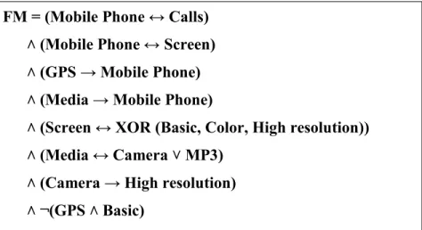
The full set of rules in a feature model can be captured in a Boolean expression. In [8] and [29], a procedure is provided for converting feature models into propositional formulas, where the features are treated as propositional variables, and the relationships are expressed in terms of conjunction ˄, disjunction ˅, negation ¬, implication →, and bi-implication ↔. Figure 3 above shows the mobile phone feature model of Figure 1 converted into a propositional formula. The last two lines represent the cross-tree constraints (CTCs) in the model.
From Figure 3 we can conclude that the total number of rules in this feature model is 16, including the following:
1. The root feature is mandatory. 2. Every child requires its own parent.
3. If the child is mandatory, then the parent requires the child. 4. Every group adds a rule about how many members can be chosen.
FM = (Mobile Phone ↔ Calls) ˄ (Mobile Phone ↔ Screen) ˄ (GPS → Mobile Phone) ˄ (Media → Mobile Phone)
˄ (Screen ↔ XOR (Basic, Color, High resolution)) ˄ (Media ↔ Camera ˅ MP3)
˄ (Camera → High resolution) ˄ ¬(GPS ˄ Basic)
5. Every cross-tree constraint (CTC) is a rule.
The total number of rules will be used as the “full correctness” score in this study, thus making “correctness” one of the optimization objectives. (see section 3.4)
Another source of feature models used in this study was the Linux Variability Analysis Tools (LVAT) feature model repository, which resulted from the works of Berger et al. [15], [87], [14], [13], [12]. The models were reverse-engineered from open-source code, comments, and documentation of such projects as the Linux kernel, eCos and FreeBSD operating systems, and other large projects. The resulting feature models had distinctly different properties than models published by academic researchers, such as those in SPLOT [68]. The LVAT models are significantly larger in size, more constrained, and have higher branching factors than academic models, but they also had lower ratios of feature groups and, in general, shallower leaves. The models downloaded from LVAT website had the DIMACS format, which expresses each model as a formula in the Conjunctive Normal Form (CNF).
2.3 Tools for Automated Analysis of Feature Models
Here we describe the conventional formula solvers (a.k.a. theorem provers) that are traditionally used for analyzing feature models. Those solvers include BDD (Binary Decision Diagram) solvers, SAT (Satisfiability) solvers, and CSP (Constraint Satisfaction Problem) solvers. We also discuss an SMT (Satisfiability Modulo Theories) solver that was more recently used for the same purpose.
2.3.1 Binary Decision Diagrams (BDD)
Binary Decision Diagrams are compact data structures for Boolean expressions widely studied in the hardware verification community [80]. A BDD is a directed acyclic graph that represents a Boolean expression.
For example, the expression (k → p)∧(p → c)
is represented by the BDD in Figure 4. [29]
Figure 4: Example Binary Decision Diagram
Using a BDD, the Boolean expression can efficiently be evaluated to find valid solutions. For instance, it is possible to test in constant time whether a BDD is constantly true or false, although for Boolean expressions this problem is NP-complete [1].
2.3.2 The Satisfiability (SAT) Problem
The problem of determining the Satisfiability of sentences in propositional logic is called the SAT problem [80]. It was the first problem proved to be NP-complete [25]. Boolean Satisfiability is a decision problem to check whether a Boolean formula
evaluates to true for any of the assignments to its variables. If there is such assignment the formula is said to be satisfiable, otherwise it is unsatisfiable. For instance, (a ∧ b) is satisfiable as witnessed by the assignment {a=true, b=true}. Formula (a ∧ b ∧ ¬a) is unsatisfiable: no value for variable a causes the formula to evaluate to true [75].
2.3.3 The Constraint Satisfaction Problem (CSP)
The constraint satisfaction problem includes a set of variables, each having a range of allowable values. A problem is solved when each variable has a value that satisfies all the constraints on the variable. CSP search algorithms enable the solution of complex problems by eliminating large portions of the search space all at once by identifying variable/value combinations that violate the constraints. [80] A CSP – in contrary to a SAT– includes constraints containing integer and interval values [69]. The algorithm to transform a feature model into a CSP was introduced in [10].
2.3.4 Satisfiability Modulo Theories (SMT)
Satisfiability modulo theories (SMT) generalizes Boolean satisfiability (SAT) by adding equality reasoning, arithmetic, fixed-size bit-vectors, arrays, quantifiers, and other useful first-order theories. An SMT solver is a tool for deciding the satisfiability (i.e. validity) of formulas in these theories. Z3 is an efficient SMT Solver freely available from Microsoft Research. It is used in various software verification and analysis applications. [31]
2.3.5 The Infeasibility of Exhaustive Search for Optimal Configuration All the methods discussed above (BDD, SAT, CSP, and SMT) are concerned with finding correct solutions to logic expressions in the shortest time possible. Nevertheless, when searching for optimal configuration options with multiple quality attributes (as in the problem addressed by this study, see section 3.1), it is required that all correct solutions be found and evaluated, which becomes an infeasible task as feature models grow in size and complexity.
For example, Pohl et al. [75], who experimented with finding solutions for feature models using BDD, SAT, and CSP solvers, ruled that the task of finding all solutions for a feature model becomes infeasible when the cardinal (number of valid solutions) is over 3 million, hence excluding feature models as small as 90 features in size.
Olaechea Velazco [96] used Z3 SMT solver to find optimal solutions to the two feature models and quality attributes that we used in [86]. For the smaller model with 43 features only, the process took 1.65 hours. As for the larger model, with 290 features, the process timed out and was stopped after 15 days. The cardinal for this 290-feature model is 2.26x1049 [75].
Other examples that show the hardness of exhaustive search for large feature models are mentioned in section 4.1.
Hence we resorted to heuristic methods for this task, namely multi-objective evolutionary algorithms (MOEAs) that are explained in the following sections.
2.4 Genetic Algorithm
All MOEA’s used in this study have Genetic Algorithm at their core. The original Genetic Algorithm (GA) was developed with a single fitness value in mind, i.e. a single optimization objective. Figure 5 lists an outline of the Genetic Algorithm, adapted from [65].
The MatingSelection() function selects individuals from the population with a probability proportionate with their fitness. An individual may, by chance, be chosen for breeding multiple times.
Initialization
popsize ← desired population size P ← {}
for popsize times do
P ← P ∪ {new random individual}
Best ← null
Repeat until Termination
for each individual Pi ∈ P do
AssignFitness(Pi)
if Best = null or Fitness(Pi) > Fitness(Best) then
Best ← Pi
Q←{}
for popsize/2 times do
Parent Pa ← MatingSelection(P)
Parent Pb ← MatingSelection (P)
Children Ca,Cb ← Crossover(Copy(Pa),Copy(Pb))
Q ← Q ∪{Mutate(Ca),Mutate(Cb)} P ← Q
Termination Best is ideal solution or we’ve run out of time
return Best
The individual solutions are of the Boolean string type. The Crossover() function performs a single-point crossover, where a point is chosen randomly, and the bits are swapped between the two parents as shown in Figure 6 [65]. Crossover between two parents is performed with a predetermined probability.
The Mutate() function performs bit-flip mutation, where each bit in the string may be flipped at a predetermined probability.
Figure 6: Example of a single-point crossover, from [22]
2.5 Multi-Objective Evolutionary Algorithms (MOEAs)
Many real-world problems involve simultaneous optimization of several incommensurable and often competing objectives. Often, there is no single optimal solution, but rather a set of alternative solutions. These solutions are optimal in the wider sense that no other solutions in the search space are superior to them when all objectives are considered [118].
Formally, we define two types of Pareto Dominance: Boolean Dominance is defined as follows: A vector u = {u1, . . . , uk} is said to be dominated by a vector
v = {v1, . . . , vk} if and only if u is partially less than v, i.e.
∀i ∈ {1, … , k}, ui ≤ vi and ∃ i ∈ {1, … , k} ∶ ui < vi (1)
whereas Continuous Dominance is measured with a continuous function, such as equation 2 in Figure 7.
The Pareto Front is the set of all points in the objective space that are not dominated by any other points.
Many algorithms have been suggested over the past two decades for multi-objective optimization based on evolutionary algorithms that were designed primarily for single-objective optimization, such as Genetic Algorithms, Evolutionary Strategies, Particle Swarm Optimization, and Differential Evolution.
The algorithms we used in this study were already implemented in the jMetal framework [34]. They are:
1. IBEA: Indicator-Based Evolutionary Algorithm [116].
2. NSGA-II: Nondominated Sorting Genetic Algorithm, version 2 [33]. 3. SPEA2: Strength Pareto Evolutionary Algorithm, version 2 [117]. 4. FastPGA: Fast Pareto Genetic Algorithm [38].
5. MOCell: A Cellular Genetic Algorithm for Multi-objective Optimization [71].
2.6 Indicator-Based Evolutionary Algorithm (IBEA)
Of the 5 algorithms listed above, IBEA achieved the best results, and that was due to its unique fitness ranking criteria. In Figure 7, we provide an outline of the IBEA algorithm. The details can be found in [116]. In the following section, we explain the
fitness ranking criteria in each of the 5 algorithms.
Input: α (population size)
N (maximum number of generations) κ (fitness scaling factor)
Output: A (Pareto set approximation)
Step 1: Initialize: Generate an initial population P of size α; and an
initial mating pool P’ of size α; append P’ to P; set the generation counter m to 0.
Step 2: Assign Fitness: Calculate fitness values of individuals in P,
i.e., for all x1∈ P set
( 1) = ∑ ( , )
∈ { } (2)
Where IHD(.) is a dominance-preserving binary indicator. Specifically:
( , 1) = { ( ( 1) ( ) 1
1) ( ), (3)
Where IH is the Hypervolume defined in section 3.6 below.
Step 3: Environmental selection: Iterate the following three steps until
the size of population P does not exceed α:
1. Choose an individual x∗∈ P with the smallest fitness value, i.e.,
F(x∗) ≤ F(x) for all x ∈ P.
2. Remove x∗ from the population.
3. Update the fitness values of the remaining individuals, i.e. F(x) = F(x) + ({ },{ }) for all x ∈ P.
Step 4: Termination: If m ≥ N or another stopping criterion is satisfied
then set A to the set of decision vectors represented by the nondominated individuals in P. Stop.
Step 5: Mating selection: Perform binary tournament selection with
replacement on P in order to fill the temp mating pool P’.
Step 6: Variation: Apply crossover and mutation operators to the
mating pool P’ and add the resulting offspring to P. Increment the generation counter (m = m + 1) and go to Step 2.
2.7 Fitness Ranking Criteria in MOEAs
All MOEAs used in this study are based on Genetic Algorithms. They share some basic qualities, such as: single-point crossover, bit-flip mutation, binary tournament for mating selection, and elitism. They also have differences, the most relevant to mention here being the ranking criterion (i.e. fitness assignment) used to determine which individuals have stronger chance to survive to the next generation. Those criteria are detailed here:
1. NSGA-II: The sorting procedure in NSGA-II is depicted in Figure 8, adopted from [33]. It shows how the combined primary population (Pt) and secondary population (Qt) gets sorted according to domination, where F1 contains all nondominated solutions; F2 contains all nondominated solutions after excluding F1 and so on. When the
solutions within F3 need to be sorted for truncation, they are ranked according to crowding distance, a value calculated from distances to nearest neighbors in all objective values. Thus diversity preservation is the second criterion to determine fitness for survival.[33]
2. SPEA2: The sorting procedure in SPEA2 is somewhat similar to that depicted in Figure 8, with two differences. First, domination sorting only takes place once, thus dividing the population into F1 and F2. Second, the ranking criterion for individuals in F2 is based on the strength of each solution, defined as the number of solutions that are dominated by it. The fitness value of a point is the sum of strengths of all solutions that dominate that point added to a density estimation that works to prioritize points with less proximity to nearest neighbors. [117]
3. FastPGA: The fitness of the nondominated solutions is calculated using the crowding distance as in NSGA-II. The fitness of dominated solution is the number of solutions it dominates, similar to SPEA2. Ranking is according to both domination and fitness. [38]
4. MOCell: The solutions are ordered using a ranking and a crowding distance estimator similar to NSGA-II. Bigger distance values are favored. [71]
5. IBEA: Equation 2 in Figure 7 shows IBEA's fitness assignment. Each solution is given a weight based on IHD(.), a dominance-preserving quality indicator, thus factoring in more of the optimization objectives of the user. The authors of IBEA, Zitzler and Kunzli, designed the algorithm such that “preference information of the decision
maker” can be “integrated into multiobjective search” [116]. It is noticed here that the ranking criteria in IBEA place no emphasis on diversity of solutions, thus diverging from the conventional trend set by NSGA-II and SPEA2, and followed by others.
2.8 Summary
In this chapter, we introduced all the background material necessary to move forward. In the majority of previous work on automated analysis of feature models, only one dimension is explored, namely the correctness dimension, such as checking the soundness of the model, and deriving correct configurations. There wasn’t enough exploration of multiple dimensions that address user preferences such as cost, reliability, etc.
Going forward, we will examine feature models with added quality attributes that express stakeholder interests, and we will use MOEAs to find near optimal feature selection that conform with the dependencies and constraints laid out in the feature models.
Chapter 3: Problem Formulation
In this chapter, we define our problem, i.e. multi-objective configuration of software product lines, and we place it within the context of related work in reasoning about feature attributes and user preferences in feature models. In addition, we highlight the relationship of this problem with interactive or “user-in-the-loop” configuration.
3.1 Problem Definition
The problem of multi-objective feature selection in software product lines in formally defined as follows.
Suppose a feature model is composed of n features, denoted as F = {F1, F2, …, Fn}, that the features are subject to a set of m constraints (including all dependencies, see Fig. 3), denoted as C = {C1, C2, …, Cm}, a set of k user objectives OSi = {OSi1, OSi2, …, OSik} where each objective is calculated for a given subset of features Si, and a search budget of T seconds. Find a group of feature subsets Si⊂ F, such that:
a- C1 = C2 = … = Cm = TRUE
b- OSi is not dominated by any OSj found up to time T, ∀ i,j (domination defined in equation 1, section 2.5).
3.2 Extending Feature Models with Attributes
The idea of extending (or augmenting) feature models with quality attributes was proposed by many, among them Czarnecki et al. [28], Zhang et al. [115] and Cordy et al.
[27]. Many researchers used feature models with attached attributes and synthetic data to experiment with optimizing feature selection in Software Product Lines, including Benavides et al. [9], White et al. [103], [104], Bagheri et al. [6] Soltani et al. [91] and Guo et al. [45] as will be detailed in section 4.2.
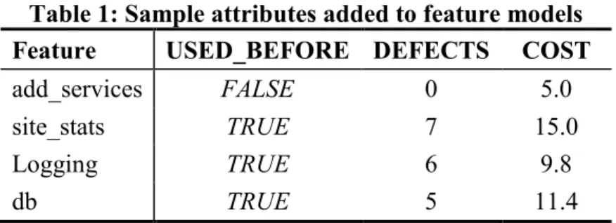
3.3 Our Approach to Assigning Feature Attributes
In order to accommodate user business concerns in the process of product customization, we augmented the feature model with 3 attributes per feature: COST, USED_BEFORE, and DEFECTS. COST takes real values distributed normally between 5.0 and 15.0, USED_BEFORE takes Boolean values distributed uniformly, and DEFECTS takes integer values distributed normally between 0 and 10. The only dependency among these qualities is:
if (not USED_BEFORE) then DEFECTS = 0 (4)
Table 1 shows a sample of the attributes given to the “Web Portal” feature model.
Table 1: Sample attributes added to feature models
Feature USED_BEFORE DEFECTS COST
add_services FALSE 0 5.0
site_stats TRUE 7 15.0
Logging TRUE 6 9.8
db TRUE 5 11.4
This provides three of the five optimization objectives: to minimize total cost, to maximize feature that were used before, and to minimize the total number of known
defects. The two remaining objectives are: to maximize correctness, i.e. minimize rule violations, and to maximize the number of offered features.
3.4 Defining the Optimization Objectives
In this work we optimize the following objectives:
1. Correctness; i.e. compliance to the relationships and constraints defined in the feature model. Since the tools we used (jMetal) treats all optimization objectives as minimization objectives, we seek to minimize rule violations.
2. Richness of features; we seek to minimize the number of deselected features. 3. Features that were used before; we seek to minimize the features that weren’t used
before.
4. Known defects; which we seek to minimize. 5. Cost; which we seek to minimize.
3.5 Why Maximize the Number of Features?
Some have looked at the second objective above and questioned its merit; does the user really seek to maximize the number of features in a product? Our answer takes a holistic look at the goal of our optimization: to provide the user with a wide range of Pareto-optimal solutions that explore as many feature configuration choices as possible, and then let the user make their own decisions. If the “feature-richness” objective is removed, the other four objectives would push the solutions toward minimizing the number of features, since that area of the decision space tends to minimize violations,
new features, known defects, and cost. Such formulation would defeat the purpose of offering a diverse set of valid products.
3.6 Quality of Pareto Front
Quality indicators can be calculated to assess the performance of multi-objective metaheuristics. In this study, we used three indicators:
1. Hypervolume (HV): defined in [118] as a measure of the size of the space covered, as follows: Let (x1, x2, …, xk) be a set of decision vectors. The hypervolume is the volume enclosed by the union of the polytopes (p1, p2, …, pk) where each pi is formed by the intersections of the following hyperplanes arising out of xi, along with the axes: for each axis in the objective space, there exists a hyperplane perpendicular to the axis and passing through the point (f1(xi), f2(xi), …, fn(xi)). In the two-dimensional (2-D) case, each pi represents a rectangle defined by the points (0,0) and (f1(xi), f2(xi)). In jMetal, all objectives are minimized, but the Pareto front is inverted before calculating hypervolume, thus the preferred Pareto front would be that with the most hypervolume.
2. Spread: defined in [33], measures the extent of spread in the obtained solutions. It is found with the formula:
r ad = d d ∑ di d̅
1 i 1
d d ( 1)d̅ ( )
where:
di is Euclidean distance among consecutive points,
d̅ is Average of di’s, and
df and dl are the Euclidean distances between the extreme and boundary solutions of Pareto front.
3. %Correct: i.e. the percentage of fully-correct solutions, which is an indicator particular to this problem. Since correctness is an optimization objective that evolves over time, there maybe points in the final Pareto front that have rule violations. Such points are not likely to be useful to the user. We are interested in percentage of points within the Pareto front that have zero violations, and thus a full-correctness score. For instance, if %Correct = 70% then we have 70 fully-compliant configurations out of 100 members of the final population.
3.7 Run Time versus Number of Evaluations; Which One Shall Be Fixed?
In [86], we compared MOEAs by allowing each to perform a fixed number of fitness function evaluations, which is the commonly used approach. The number of evaluations is proportional to the total run time and the required CPU power. Yet, the total run time is affected by many other algorithm-dependent operations, including the fitness ranking of individuals in each generation. This leads to varying runtimes with the same number of evaluations. For instance, we noticed that IBEA took five times longer than NSGA-II to perform 50K evaluations on 5 objectives for the E-Shop feature model,
which meant that IBEA spent far more time in fitness ranking than NSGA-II. This was expected from our study of the fitness ranking criterion in section 2.7.
The question here is: which criterion shall we fix in order to have a fair comparison among algorithms? We have come to the opinion that each algorithm should be given a fixed amount of time to calculate its best approximation of the Pareto front. A better algorithm should score better on the quality indicators (HV, Spread, %correct) within that duration of time. Going back to the comparison between IBEA and NSGA-II, if both are given the same duration of time, then NSGA-II would perform far more evaluations than IBEA, and thus would be given a better chance to improve its results. As we will see in the coming section, providing NSGA-II with the chance to evolve more generations did not help it to overcome IBEA at producing more correct solutions or better HV.
In addition, the user should be more concerned with the amount of time it takes to optimize, than with the number of evaluations. CPU power is often available at the user’s disposal, and the algorithms should utilize that CPU power to produce the best results in the least amount of time, regardless of number of evaluations or number of evolved generations.
Therefore, in the this paper’s experiments we make our comparisons of the results after limiting the amount of time given to each algorithm, regardless of number of evaluations each algorithm were able to perform.
3.8 Relationship with Interactive Configuration
This problem of feature selection in software product lines has the most practical application in user-interactive tools for product configuration. Such tools usually begin with the “bare-bone” product, which has the essential or mandatory features, then allows the user to fix some of the optional features, and makes recommendations regarding the choices to make next. The user may also be prompted to limit the objective space to the levels that they can afford, such as a maximum cost. The tool would periodically take user input and run optimization cycles and come back with recommendations. Multi-objective approaches are best suited for this paradigm since they provide the user with a set of Pareto-optimal choices each with its own trade-offs.
The problem that we attempt to solve in this paper is the most complex form of user-interactive configuration, since we deal with optimum feature selections before the user makes any feature choices or limits the objective space. As the user makes periodic choices, the space of options becomes smaller and smaller, and the tools would perform faster than in the most general case.
Chapter 4: Related Work
4.1 Automated Analysis of Feature Models
In [75], a large experiment was performed to measure the efficiency of available BDD, SAT and CSP solvers to perform four analysis operations on 90 feature models from the SPLOT repository. They reported long run times for certain operations, and they cancelled certain runs with the larger feature models when the run time exceeded three hours. An exponential runtime increase with the number of features for non-BDD solvers on the “valid” operation was also reported. The “product enumeration” operation was not attempted for feature models with more than 3 million valid products, since this operation was not feasible. This left out the largest 12 models out of 90, and thus the remaining models were all below 90 features in size.
In [64], a basic search method (Breadth-First Search) is used to find feature model inconsistencies and suggest fixing sets. The method was run with 60 feature models from the SPLOT website, the largest being 94 features. They report that computation time increases steadily as the number of features increases; for instance, the operation took about 27 minutes for a size of 94 features.
In [70], efficient ordering heuristics are proposed for BDDs that represent feature models. Such ordering can dramatically reduce the size of BDDs, thus allowing fast processing for interactive configuration algorithms. The proposed heuristics were tested
with five realistic feature models, in addition to randomly-generated feature models with larger sizes. It was shown that the heuristics produce high quality variable orders that enable the compilation of large feature models with up to 2,000 features.
In [69], it is shown that the task of satisfiability (SAT) solving of realistic models is easy. In particular, the phenomenon of phase transition is not observed for realistic feature models. The explanation for this is that many real world problems are either over-constrained (in terms of variability: they have no realizable products) or under-constrained (they have many easily identifiable realizations). For instance, consistency checks on randomly-generated models with up to 10,000 features and a large number of cross-tree constraints took about 0.4 seconds. In addition, computing valid domains was completed in about 22 seconds for models with 5,000 features and a fairly large number of cross-tree constraints.
The only two studies we know that experimented with the LVAT (Linux Variability Analysis Tools) feature models were done by Johansen et al. [55] who generated test covering arrays for feature models, and Henard et al. [54] who worked on prioritizing t-wise test suites. Both experimented with three very large models from the LVAT repository (Linux, eCos, and FreeBSD), in addition to models from SPLOT and other sources. All of the experiments in [55] timed out for the largest model (Linux Kernel with 6888 features), and some timed out for even smaller models. In [54], the 6-wise coverage experiment took 20 hours for the Linux Kernel feature model.
4.2 Optimizing Feature Models with Attributes
The idea of extending (or augmenting) feature models with quality attributes was proposed by many, among them Czarnecki et al. [28], Zhang et al. [115] and Cordy et al. [27]. The following papers used feature models with attached attributes and synthetic data to experiment with optimizing feature selection in Software Product Lines.
Benavides et al. [9] assigned feature attributes such as price range and time range. They modeled the problem as a Constraint Satisfaction Problem, and solved it using CSP solvers to return a set of features which satisfy the stakeholders’ criteria. Clearly, they converted a multi-objective optimization problem into single-objective by combining all the objectives in one formula. They experimented with small models of sizes up to 25 features, and experienced exponentially increasing runtimes.
White et al. [103] used feature attributes related to resource consumption, cost and accuracy. They mapped the feature selection problem to a multidimensional multi-choice knapsack problem, and apply Filtered Cartesian Flattening to provide partially optimal feature selection. Then in [104], they introduced the MUSCLE tool, which provided a formal model for multistep configuration and mapped it to constraint satisfaction problems (CSPs). Hence, CSP solvers were used to determine the path from the start of the configuration to the desired final configuration. A sequence of minimal feature adaptations is calculated to reach from the initial to the desired feature model configurations.
helps to rank and select the most relevant high level business objectives for the target stakeholders (e.g., security over implementation costs), and then helps to rank and select the most relevant features from the feature model to be used as the starting point in the staged configuration process.
Soltani et al. [91] annotated features with business concerns and attached a cost to each feature, then employed Hierarchical Task Network (HTN) planning to automatically select suitable features that satisfy the stakeholders’ business concerns and resource limitations.
Shi et al. [88] utilize a knapsack approximation algorithm along with greedy search and a constraint solver to select features based on customer requirements. They experiment with randomly-generated feature models with various sizes.
More recently, Guo et al. [45] augmented feature models with attributes such as memory and CPU usage, and used a Genetic Algorithm to provide an optimum feature selection, thus aggregating all objectives into one formula with preset weights.
In all the works mentioned above (sections 4.1 and 4.2), the testing was done with relatively small feature models published in academic repositories like SPLOT, or with large feature model that were randomly-generated based on the same characteristics as SPLOT models. Large feature models that represent actual code (such as those published in LVAT) have not yet been used to test out automated analysis and configuration methods.
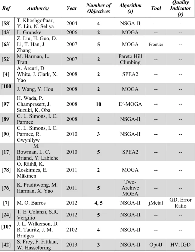
4.3 Pareto-Optimal Search-Based Software Engineering
This section is extracted from a recent survey by Sayyad and Ammar [82].
Historically, the field of Search-Based Software Engineering (SBSE) has seen a slow adoption of Pareto optimization techniques, generally known as multiobjective optimization techniques. Back in 2001, when Harman and Jones coined the term SBSE [48], all surveyed and suggested techniques were based on single-valued fitness functions. In 2007, Harman commented on the current state and future of SBSE [47], and in the “Road-map for Future Work” section he suggested using multiobjective optimization. Then in 2009, Harman et al. [50] were able to cite several works in which multiobjective optimization techniques were deployed. Still, most of the work reviewed therein, as well as work done thereafter, optimized two objectives only, while higher numbers appeared only occasionally. Also, the typical tendency was to use algorithms that are popular in other domains, such as NSGA-II and SPEA2. In this survey, we attempt to systematically identify these trends.
Several surveys and review papers were published in the field of SBSE [47], [50], [51], [30]. Some surveys focused on subfields, such as search-based software design [77], and search-based test data generation [67]. This survey is the first of its kind, in which we survey SBSE research work that employed Pareto optimization techniques.
The total number of surveyed papers was 51. Figure 9 breaks them down by area of application, while Figure 10 classifies them by year of publication.
Figure 9: Pareto-Optimal SBSE papers by area of application
Tables 2-5 list all the surveyed papers, along with the multiobjective algorithms, the number of objectives, tools and quality indicators. The surveyed papers are divided according to the application areas of software requirements, design, testing, and management. 0 2 4 6 8 10 12 14 16
Requirements Design Testing Management various
0 2 4 6 8 10 12 14 2 0 0 4 2 0 0 5 2 0 0 6 2 0 0 7 2 0 0 8 2 0 0 9 2 0 1 0 2 0 1 1 2 0 1 2 2 0 1 3
Table 2: List of surveyed Pareto-Optimal SBSE works in software requirements
Ref Author(s) Year Number of Objectives Algorithm (s) Tool Indicator Quality (s) [114] Y. Zhang, M. Harman, S. A. Mansouri 2007 2 NSGA-II, Pareto GA -- -- [41] A. Finkelstein, M. Harman, S Mansouri, J Ren, Y Zhang 2008 2 NSGA-II -- --
[36] J. J. Durillo, Y. Zhang, E. Alba, A.
J. Nebro 2009 2
NSGA-II,
MOCell jMetal Spread HV, [113] Y. Zhang, E. Alba, J. J. Durillo, S.
Eldh, M. Harman 2010 3 NSGA-II -- -- [35] J. J. Durillo, Y. Zhang, E. Alba, M. Harman, A. J. Nebro 2011 2 NSGA-II, MOCell, PAES jMetal HV, Spread [18] M. M. A. Brasil, T. G. N. da Silva, F. G. de Freitas, J. T. de Souza, M. I. Cortés
2011 3 NSGA-II, MOCell jMetal Spread HV,
[53] W. Heaven, E. Letier 2011 2 NSGA-II Matlab -- [95] V. Veerappa, E. Letier 2011 2 Clustering Matlab GA with -- [60] A.C. Kumari, K. Srinivas, M.P.
Gupta 2012 2 QEMEA -- HV, Spread, Convergenc e [86] A. S. Sayyad, T. Menzies, H. Ammar 2013 2, 3, 4, 5 IBEA, NSGA-II, ssNSGA-II, SPEA2, FastPGA, MOCell, MOCHC jMetal Spread HV,
Table 3: List of surveyed Pareto-Optimal SBSE works in software design
Ref Author(s) Year Number of Objectives Algorithm (s) Tool Indicator Quality (s) [58] T. Khoshgoftaar, Y. Liu, N. Seliya 2004 4 NSGA-II -- --
[43] L. Grunske 2006 2 MOGA -- --
[63] Z. Liu, H. Guo, D. Li, T. Han, J.
Zhang 2007 5 MOGA
Frontier -- [52] M. Harman, L. Tratt 2007 2 Pareto Hill Climbing -- --
[4] A. Arcuri, D. White, J. Clark, X.
Yao 2008 2 SPEA2 -- --
[100
] J. Wang, Y. Hou 2008 2 MOGA -- --
[97] H. Wada, P. Champrasert, J.
Suzuki, K. Oba 2008 10 E
3-MOGA -- -- [89] C. L. Simons, I. C. Parmee 2008 2 NSGA-II -- -- [90] C. L. Simons, I. C. Parmee, R.
Gwynllyw 2010 3 NSGA-II -- --
[17] Bowman, L. C. M.
Briand, Y. Labiche 2010 5 SPEA2 -- -- [78] O. Räihä, K. Koskimies, E.
Mäkinen 2011 2 MOGA -- --
[76] K. Praditwong, M. Harman, X. Yao 2011 5 Archive
Two-MOEA -- --
[7] M. O. Barros 2012 4, 5 NSGA-II jMetal GD, Error Ratio [24] T. E. Colanzi, S.R. Vergilio 2012 5 NSGA-II -- -- [107
]
J. L. Wilkerson, D. R. Tauritz, J. M.
Bridges 2102 4 NSGA-II -- --
Table 4: List of surveyed Pareto-Optimal SBSE works in software testing
Ref Author(s) Year Number of Objectives Algorithm (s) Tool Indicator Quality (s) [109] S. Yoo, M. Harman 2007 2, 3 vNSGA-II NSGA-II, -- --
[49] M. Harman, K. Lakhotia, P.
McMinn 2007 2 NSGA-II -- --
[101] Z. Wang, K. Tang, X. Yao 2008 2, 3 NSGA-II, MODE -- -- [66] C. Maia, R. Carmo, F. Freitas, G.
Campos, J. Souza 2009 3 NSGA-II jMetal -- [108] T. Yano, E. Martins, F. Sousa 2010 2 M-GEOvsl -- --
[73] G. H. L. Pinto, S. R. Vergilio 2010 3 NSGA-II -- -- [61] W. Langdon, M. Harman, Y. Jia 2010 2 NSGA-II -- -- [110] S. Yoo, M. Harman 2010 2, 3 HNSGA-II -- -- [102] Z. Wang, K. Tang, X. Yao 2010 2, 3 HaD-MOEA NSGA-II, -- HV
[20] R. Cabral, A. T. R. Pozo, S. R. Vergilio 2010 2 Pareto Ant Colony -- -- [23] T. E. Colanzi, W. Assuncao, S. R. Vergilio, A. Pozo 2011 2 NSGA-II, SPEA2 jMetal GD, ED [5] W. K. G. Assunção, T. E. Colanzi, A. T. R. Pozo, S. Vergilio 2011 4 NSGA-II, SPEA2 jMetal GD, IGD, Coverage, ED [112] S. Yoo, R. Nilsson, M. Harman 2011 3 Two-Arch-ive MOEA -- -- [111] S. Yoo, M. Harman, S. Ur 2011 2 NSGA-II jMetal --
[39] J. Ferrer, F. Chicano, E. Alba 2011 2
NSGA-II, SPEA2, PAES, MOCell, Random jMetal HV, attain-ment surfaces
![Figure 1, adapted from [11], depicts a simplified feature model inspired by the mobile phone industry](https://thumb-us.123doks.com/thumbv2/123dok_us/11081087.2994618/24.918.209.750.481.836/figure-adapted-depicts-simplified-feature-inspired-mobile-industry.webp)
![Figure 5: Genetic Algorithm, adapted from [22]](https://thumb-us.123doks.com/thumbv2/123dok_us/11081087.2994618/31.918.222.707.520.995/figure-genetic-algorithm-adapted-from.webp)
![Figure 8: NSGA-II sorting procedure, from [13]](https://thumb-us.123doks.com/thumbv2/123dok_us/11081087.2994618/35.918.286.726.196.493/figure-nsga-ii-sorting-procedure-from.webp)